Chapter 15

Time-independent Perturbation Theory

15.1  INTRODUCTION

We have seen in the first part of the book that it is possible to solve Schrodinger equation exactly (i.e., the energy eigenvalues and eigenfunctions may be found exactly) for a particle in potential like harmonic potential or Coulomb potential. However, many a times, there are situations in which the potential is deviating a bit from the potentials for which Schrodinger equation may be solved exactly. For example, if a particle is put in a potential, deviating from harmonic potential, that is, if potential is it is not possible to find exact eigenvalues and eigenfunctions of this so-called anharmonic potential. But it is possible to find approximate solutions of the Schrodinger equation when (in the above example) the potential is deviating from the harmonic potential by only small amount, that is, when constants a and b (appearing in the above mentioned potential) are very small. In this chapter, we shall develop time-independent perturbation theory which shall give approximate eigenvalues and eigenstates of the system that have potential differing by small amount from the standard potential for which Schrodinger equation may be solved exactly.

15.2  NON-DEGENERATE PERTURBATION THEORY

The perturbation theory, which we are going to discuss in this Chapter, is applicable when following criteria are satisfied:

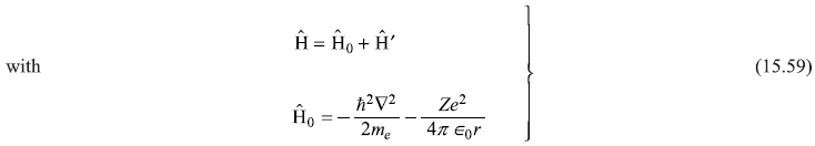
1. The total Hamiltonian of the system may be written as the sum of two parts.

    

   Ĥ = Ĥ₀ + Ĥ′        (15.1)

    

2. The eigenvalues and eigenstates of the so-called unperturbed Hamiltonian Ĥ₀ are known, and
3. The second part of the total Hamiltonian, Ĥ′ (Ĥ′ is known as perturbation) is much smaller, in comparison to the unperturbed Hamiltonian Ĥ₀ (as we proceed, the criterion that decides the smallness of Ĥ′ will become clear).

   The last criterion is equivalent to the underlying assumption:

4. The eigenvalues and eigenstates of the total Hamiltonian Ĥ do not differ appreciably from those of the unperturbed Hamiltonian Ĥ₀.

   We start with the Schrodinger equation for the unperturbed Hamiltonian

where eigenvalues and eigenstates are known. For example, Ĥ₀ may represent the Hamiltonian of a particle in a one-dimensional harmonic potential, for which (as seen in Chapter 6) we know eigenvalues and eigenstates . Here, our aim is to develop a method to solve the Schrodinger equation for the total Hamiltonian Ĥ, that is,

 

 

As mentioned earlier, it may not be possible to solve Eq. (15.3) exactly, therefore, our aim is to obtain approximate expressions for E_n and ψ_n.

Now, owing to smallness of Ĥ′, E_n, and ψ_n may not be differing much from and and, therefore, it is possible to write

where ∆ψ_n and ∆E_n are small corrections to and , respectively. Perturbation theory is all about to find these small corrections for given small perturbation potential Ĥ′. In what follows, we rewrite Ĥ′ as λĤ′, where λ is a dummy variable and may be given any small value between 0 and 1. The time-independent Schrodinger equation, whose solution we seek, then, is

 

 

Since as λ → 0, it is consistent to express ψ_n(Ε_n) in the form of a series in powers of λ with its leading term as

Here the superscripts 0, 1, 2, ... refer to the order of the perturbation. The parameter λ may take a continuous range of values between 0 and 1, and we shall set λ = 1 in the final result. Substituting the expansion of ψ_n and E_n [Eqs (15.6) in Eq. (15.5)], we get

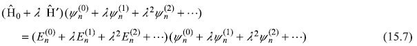
Since this equation is to be true for all values of λ (in the interval [0, 1]), the coefficients of equal powers of λ on both sides of this equation have to be equal. Equating the terms independent of λ, we have

Next, equating the coefficients οf λ give

while coefficients of λ² give

and so on.

15.2.1  The First-order Correction

We know that the eigenstates of unperturbed Hamiltonian Ĥ₀ form a complete (orthonormal) set. Therefore, each term in Eq. (15.6a) may be expressed as a linear combination of the functions . For considering first-order correction, let us express in terms of as

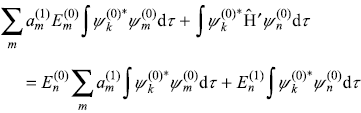
Here are the expansion coefficients to be determined. Substituting the expansion (15.8) in Eq. (15.7b), we get

or

Here we have used Eq. (15.2) in writing the first term on L.H.S. of Eq. (15.9). Let us multiply the above equation from left by and integrate over the entire allowed space, we get

or

or

or

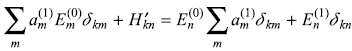
where orthonormality of the set {} dictates

and is the matrix element given as

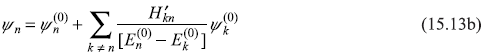
For k ≠ n, Eq. (15.10) gives

and for k = n

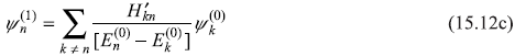
is the first-order correction to eigenvalue E_n under the perturbation Ĥ′. Putting value of coefficient from Eq. (15.12a) in Eq. (15.8), we get value of , the first-order correction to eigenstate ψ_n,

Therefore, we may conclude that the eigenvalue and eigenstate to first order are:

15.2.2  The Second-order Correction

The second-order correction to the eigenstate, , may be expanded as a linear combination of the complete set of orthonormal eigenstates of Hamiltonian Ĥ0, as

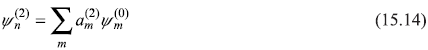
Substituting Eqs (15.14) and (15.8) in Eq. (15.7c), we have

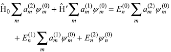
Multiplying the above equation from left by and integrating, we get

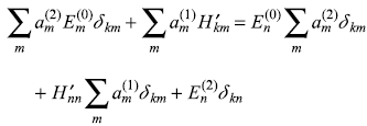
or

15.2.2.1  Second-order Correction to Eigenvalues

For k = n, we have from Eq. (15.15)

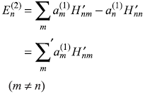
or

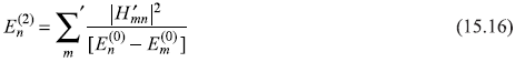
Last expression has been obtained by using expression for from Eq. (15.12a). Here we have used the relation

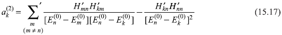
15.2.2.2  Second-order Coefficients

For k ≠ n, we get from Eq. (15.15)

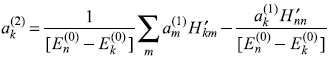
Putting the value of from Eq. (15.12a), it gives

15.3  HARMONIC OSCILLATOR SUBJECT TO PERTURBING POTENTIAL

Before proceeding further to discuss perturbation theory applicable to degenerate states, let us apply the results of non-degenerate perturbation theory to a simple case of one-dimensional harmonic oscillator subject to a small perturbing potential. Let us consider a one-dimensional harmonic oscillator described by the Hamiltonian.

which is perturbed by a small anharmonic potential

 

 

We shall consider various forms of the perturbing potential [e.g., g(x) = bx and g(x) = bx²]. We have to find the first and second-order corrections to the unperturbed energy eigenvalues of Hamiltonian Ĥ₀; the unperturbed eigenvalues and eigenstates are given by the Schrodinger equation

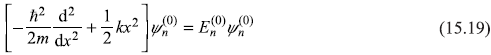
In Chapter 6, the equation was solved and the results for and were obtained as

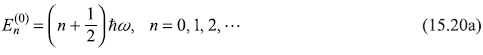
where

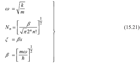
In the language of the creation and annihilation operators a^† and a, and bra and ket notations of eigenstates, the Eqs (15.18a) and (15.19) may be written as (see Chapter 8)

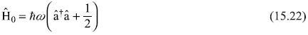
with

15.3.1  Perturbing Potential Varying as x

As a simple case, firstly, we consider the perturbing potential

 

 

The first-order correction to the unperturbed eigenvalue of state is

Putting value of x from Eq. (15.25), we get

Using the rules of operation of â and â^† on eigenket viz.

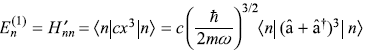
we can easily check that

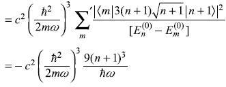
The second-order correction to E_n is

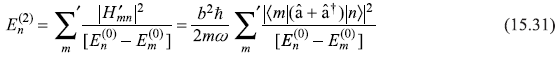
or

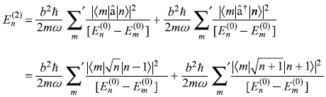
Noting that the matrix elements

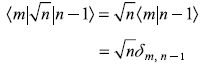
and

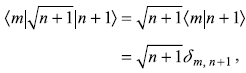
we get

or

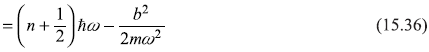
The dimensions of constant b (in the perturbing potential bx) are such that the quantity (b²/2mω³ħ) is dimensionless. Let this small dimensionless quantity be denoted by α. So,

As a result, the new energy levels of the perturbed oscillator are

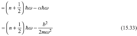
The new energy levels are simply the old energy levels, each shifted downwards by (same amount) (b²/2mω²), as shown in Figure 15.1.

In fact, the Schrodinger equation corresponding to the Hamiltonian

 

may be solved exactly. We may re-write Eq. (15.34) as

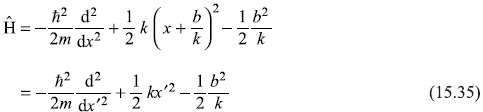
with the change of coordinate x′ = x + (b/k)

Now, Eq. (15.35) is representing the Hamiltonian of a harmonic oscillator with same force constant k and same frequency ω as that with Ĥ0 but with shifted origin of coordinate and of energy. Therefore, the solution of Schrodinger equation corresponding to the Hamiltonian equation (15.35) gives exact result:

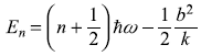
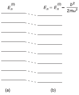
Figure 15.1 Energy levels of a one-dimensional harmonic oscillator (a) Unperturbed (b) Perturbed by the potential V′(x) = bx (up to second order)

Comparing Eqs (15.33) and (15.36) we observe that our second-order perturbation correction, in fact, gives exact results of energy levels of harmonic oscillator perturbed with linear potential.

The fact that perturbation theory gives same result as obtained by exact solution of the Schrodinger equation for linearly perturbed harmonic oscillator, clearly validates the perturbation theory. Let us mention here that it is generally not possible to solve Schrodinger equation for perturbed system, exactly, as mentioned in Section 15.1. For example, if the perturbation potential is Ĥ′ = cx³, it is not possible to solve the corresponding Schrodinger equation exactly. We study this case in the following sub-section.

15.3.2  Perturbing Potential Varying as x³

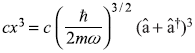
Let us next consider the one-dimensional harmonic oscillator subject to a small perturbing potential

 

 

Using Eq. (15.25), we may write x³ term as

Making use of the operator relations

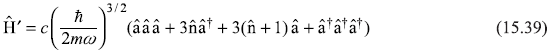
(â + â^†)³ may be written as

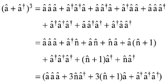
So the perturbation term is

The first-order correction

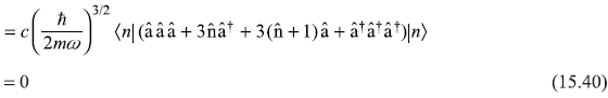
The four terms of second-order correction may be written as

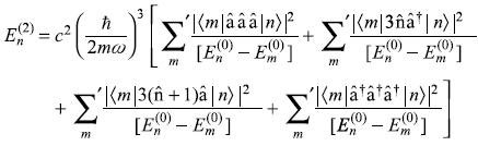
First term

Second term

Third term

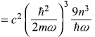
Fourth term

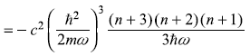
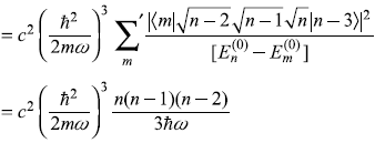
So

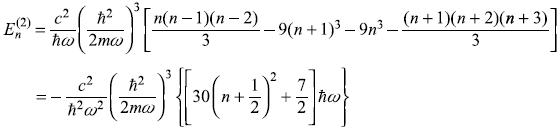
where dimensionless quantity A is

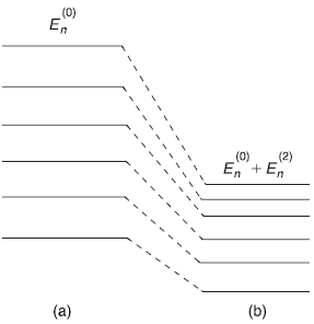
Figure 15.2 Energy levels of a one-dimensional harmonic oscillator (a) Unperturbed (b) Perturbed by the potential V′(x) = cx³ (up to second order)

In Figure 15.2, we show, schematically, the unperturbed as well as the perturbed energy levels. We observe that the effect of Ĥ′ is to lower all the unperturbed energy levels, whatever be the sign of constant c appearing in Ĥ′. Also we notice that larger the n, larger is the amount by which is lowered by perturbation.

15.4  DEGENERATE PERTURBATION THEORY

Many a times, we encounter a situation where the unperturbed states are degenerate. In fact, if the potential in which a particle moves, contains symmetry, many of the resulting eigenstates are degenerate. For example, in hydrogen atom, where the electron moves in a spherically symmetric potential, we get, for instance, three-fold degenerate p-states, five-fold degenerate d-states, and so on. In case of q-fold degenerate states, q different eigenstates of the system have same energy eigenvalue. However, if the symmetry of the potential producing q-fold degeneracy is destroyed by applying a small perturbation Ĥ′, the degeneracy is (partly or fully) removed, that is, the different eigenstates that have same energy eigenvalues in absence of perturbation may now have different energies, [shown schematically in Figure (15.3)].

The perturbation theory developed in Section 15.2 shall not be applicable to the case of degenerate states. For example, Eqs (15.12c) and (15.16) may diverge in case of degenerate states. Therefore, there is no reason to trust even the first-order correction to energy [Eq. (15.12b)] for the degenerate case. We have to look for an alternative method to deal with degenerate states. In this section, we describe the perturbation method for degenerate states.

15.4.1  Two-fold Degeneracy

Let us consider a system, which when unperturbed has two of its eigenstates and with same energy eigenvalue E⁽⁰⁾,

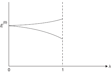
Figure 15.3 Lifting the two-fold degeneracy by a perturbation

and

With and both normalized. It may be easily seen that any linear combination of those states

where c₁ and c₂ are arbitrary constants, is also an eigenstate of Ĥ₀, with same eigenvalue E⁽⁰⁾, that is,

 

 

Generally, the perturbation λ Ĥ′ lifts the two-fold degeneracy. As shown schematically in Figure 15.3, the unperturbed energy E⁽⁰⁾ splits into two values as λ increases from 0 to 1. It is not clear, to begin with, which initial unperturbed state should be taken (i.e., what values of constants c₁ and c₂ should be taken) for implementation of the perturbation. So we start with arbitrary (but adjustable) constants c₁ and c₂ in ψ⁽⁰⁾). We want to solve the Schrodinger equation

 

 

with

 

 

Putting these expansions of E and ψ in Eq. (15.46) and collecting coefficients of equal powers οf λ, we get

 

 

Equating the terms independent of λ, we have

 

 

Next, equating the coefficients of λ gives

 

 

Putting the expansion (15.44) of ψ⁽⁰⁾ in the above equation gives

Multiplying above equation from left by and integrating over the allowed space, we get

As Ĥ₀ is Hermitian operator, the Hermitian conjugate of Eq. (15.43a) gives

which gives

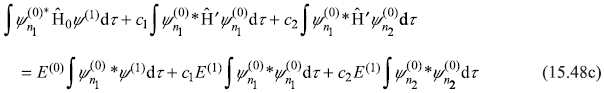
that is, the first term on L.H.S. of Eq. (15.48c) cancels the first term on its R.H.S. Then Eq. (15.48c) results in

where

and where we have used the orthogonality condition (15.43c).

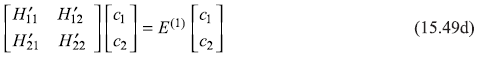
Again, multiplying Eq. (15.48b) from left by and integrating, we get

Equations (15.49a) and (15.49c) may be put in matrix form as

which has a non-trivial solution if the characteristic determinant vanishes, giving the secular equation

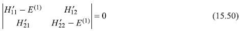
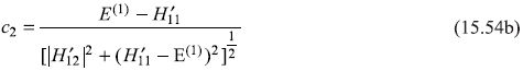
From this, we get

or

or

It may be noted here that the quantities appearing in Eq. (15.51) for the expression of are in principle known as these are just “matrix elements” of Ĥ′ (the given perturbation potential) with respect to the known unperturbed eigenstates and . So, on perturbation, the unperturbed energy E⁽⁰⁾ changes to

thereby lifting the two-fold degeneracy (if and are different).

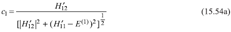
Let us, next, proceed to find the coefficients c₁ and c₂. We start with the two equations in c₁ and c₂ [Eqs (15.49a) and (15.49c)].

along with the normalization condition [on ψ⁽⁰⁾ Eq. (15.44)]

It is straightforward to find values of c₁ and c₂ from above three equations as

It may be noted here that as E⁽¹⁾ has two different values and (giving rise to different values to energy), the coefficients c₁ and c₂ shall also have two different set of values: and (for value ) and and (for value ). Therefore, the wave function

corresponds to the perturbed energy and the wave function

for perturbed energy .

15.4.2  g-Fold Degeneracy

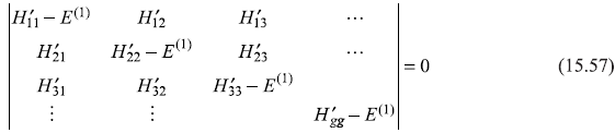
The method of previous section may be easily generalized to the case when an energy level is g-fold degenerate. As we saw in the case of two-fold degeneracy, E⁽¹⁾’S are nothing but the eigenvalues of the 2 × 2 H′ -matrix [Eq. (15.49d)]. Equation (15.50) is the corresponding characteristic equation for this matrix and, in fact, the linear combination of the unperturbed states are the eigenvectors of Ĥ′. So, in case of g-fold degeneracy, we should look for the eigenvalue equation

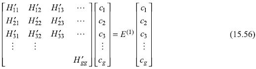
which, for nontrivial solutions, give the secular equation.

15.5  THE STARK EFFECT

As an example of the application of degenerate perturbation theory, let us consider how a uniform time-independent electric field affects the energy levels of hydrogen atom. The corresponding change in frequency of the associated spectral lines, as a result of the applied uniform electric field is called the stark effect.

Let us consider a hydrogenic atom with nuclear charge Ze in a uniform time-independent electric field E = E e_z, pointing in z-direction. The potential energy of the electron of charge –e in this field is

 

 

The total Hamiltonian of the one-electron atom in this electric field is

We know from Chapter 10 that the energy eigenvalue equation of the unperturbed atom

or

gives eigenstates which are n²-fold degenerate. We shall see in this section how the perturbing uniform electric field E removes (partly) this degeneracy. Let us, specifically, consider the four-fold degenerate n = 2 states, all with same unperturbed eigenvalue (see Section 10.8.1).

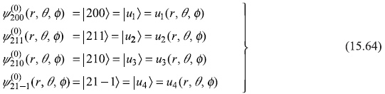
The four eigenstates corresponding to n = 2 are given as (see Section 10.8)

1. n = 2, l = 0, m = 0
   
2. n = 2, l = 1, m = 1
   
3. n = 2, l = 1, m = 0
   
4. n = 2, l = 1, m = – 1
   

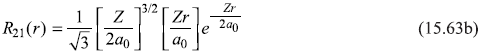
where

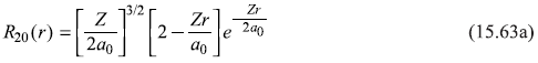
and

Let us use following shorthand notations for the four states:

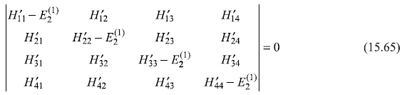
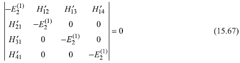
To calculate the change in energy , we must solve the corresponding secular equation [see Eq. (15.57)].

where

Now we have two observations: (1) For a system with symmetric potential, that is, for a potential with property V(r) = V (–r), the eigensates are either symmetric or anti-symmetric in position co-ordinates. In other words, the eigenstates have definite parity: even parity or odd parity. The electron in hydrogenic atom has spherically symmetric potential and, therefore, its eigenstates are with even or odd parity. The eigenstates are, in fact, even for the azimuthal quantum number l even and odd for l odd. So eigenstate has even parity and states have odd parity. (2) The perturbation Ĥ′ = |e|Ez = |e| Ercosθ is an odd function (under space inversion).

On these counts, the matrix element is non-zero if and have opposite parity; only for these cases, the integrand of the corresponding integral,

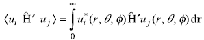
is an even function. The matrix elements

So secular equation (15.65) gives

Now we know that z commutes with and, therefore, commutes with , that is,

Taking matrix elements of both sides of Eq.(15.68) in between states and we have

or,

or

So

For n₁ = 2, l₁ = 0, n₂ = 2, l₂ = 1, we have

Therefore, we get

and Eq. (15.67) gives

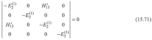
So the only non-vanishing matrix element is

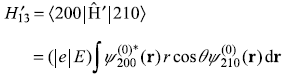
Putting values from Eqs (15.62) and (15.63), we get (for hydrogen atom Z = 1)

 

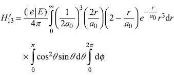
Putting these values in Eq. (15.71) gives

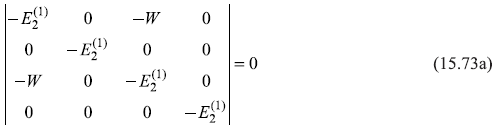
which gives four values of

Thus to first order, the four-fold degenerate n = 2 states of hydrogen atom split into three different energies, as shown schematically in Figure 15.4.

Let us now proceed to find out the new (i.e., the perturbed) eigenstates with corresponding energy eigenvalues and . We express the perturbed eigenstates ψ⁽⁰⁾ in terms of

the four (unperturbed) states and as

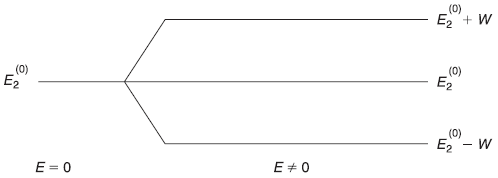
Figure 15.4 Splitting of n = 2 levels of hydrogen atom in the presence of a homogeneous electric field E

where coefficients c₁, c₂, c₃, c₄ are determined by the matrix equation [see general matrix equation (15.56)].

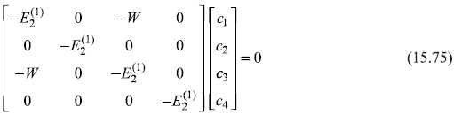
which gives four equations

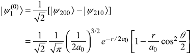
For we get c₁ = –c₃, c₂ = c₄ = 0 and Eq. (15.74) gives the required eigenstate as

Similarly for , we get c₁ = c₃, c₂ = c₄ = 0 and the corresponding eigenstate is

However, for the case of , we get c₁ = c₃ = 0 and c₂ and c₄ are arbitrary. So we may write,

with

We notice here that the perturbing electric field mixes the m = 0 states and forming two different states and with perturbed energies and respectively. On the other hand, the m = 1, –1 states and are left degenerate with unchanged energy .

15.6  THE FINE STRUCTURE OF HYDROGEN

While finding energy eigenvalues and eigenstates of hydrogen atom, we considered the Hamiltonian,

where m_e represents the reduced mass of electron. In fact, by replacing the electron mass by the reduced mass in Eq. (15.77), we have already taken into account the correction because of the motion of proton (nucleus) around the centre of mass of proton and electron. There are still more factors which, really, affect the eigenvalues and eigenstates of the electron in hydrogen atom. We mention here, in brief, these effects starting with the most significant.

1. Most significant of these effects is the so-called fine structure. In fact, the fine structure arise due to two different mechanisms: (a) due to relativistic correction (variation of electron mass with the velocity) and (b) due to spin–orbit interactions. Both of these effects produce changes in the energy levels which are relatively small. The relative changes are of the order of α², where α[= (e²/4π∊₀hc) ≈ (1/137)] is the famous fine structure constant. In this section, we will study only the effect of spin-orbit interactions towards fine structure.
2. In the quantum mechanical treatment of electromagnetic field, there are zero-point energy states [just like the residual energy of a quantum harmonic oscillator, which is called its zero-point energy (Chapter 6)]. The ever-present so-called vacuum fluctuations of electrodynamic field produce a small change in energy levels of electrons in atom. This is called the Lamb shift and is relatively of order α³.
3. The magnetic interaction between the spin magnetic moment of electron and that of proton, produces changes in the energy levels, which are of the order of (m_e/m_p)α⁴, and give rise to what is known as the hyperfine structure.

In this section, we shall consider the fine structure due to spin–orbit interactions. In order to understand the spin–orbit interaction, we consider a simple classical model of the electron orbiting around the nucleus. Let us imagine an observer at rest with the orbiting electron. From the observer’s point of view, the nucleus is circling around him (and the electron) [see Figure (15.5)].

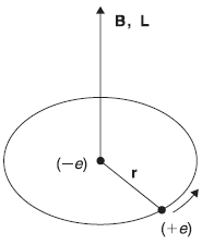
Figure 15.5 Hydrogen atom seen in electron’s frame of reference

The circulating positive charge, which constitutes a current in the orbit, sets up a magnetic field B at the electron

with effective current I = e/T (e is proton charge and T is period of the orbit). Now, in the rest frame of the proton, the orbital angular momentum of the electron is given as

From Eqs (15.78) and (15.79), we have

as B and L point in the same direction. Now, we already know that the magnetic moment vector μ associated with the electron spin angular momentum vector S is given as

Therefore, the electron with its spin magnetic moment μ_s is present there in the magnetic field B due to proton. The interaction energy of μ_s in field B is

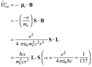
Actually this is not correct. In fact, the rest frame of electron is not an inertial frame (but an accelerating frame) as the electron is orbiting around the nucleus. This fact produces the so-called Thomas precession effect and reduces the interaction energy by a factor of 2. Thus the correct interaction is

This spin–orbit interaction is due to the torque exerted on the spin magnetic moment μ_s of the electron by the magnetic field B of the proton in the electron’s instantaneous rest frame.

As we had seen in Section 13.2, the orbital angular momentum operator and the spin angular momentum operator Ŝ do not commute with the total Hamiltonian . However, the total angular momentum operator and commute with Ĥ. Therefore, these quantities are conserved. In other words, the eigenstates of and are simultaneous eigenstates of total Hamiltonian Ĥand may be used in the perturbation theory.

As the Hamiltonian contains spin–orbit interaction, the wave function of the electron should contain both the space as well as spin part. So it will be most appropriate to write electron states in terms of Pauli wave functions.

The Pauli wave functions of the unperturbed Hamiltonian Ĥ₀, written in Pauli operator form as

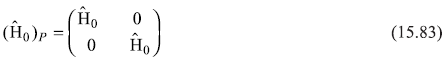
are

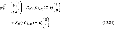
Pauli wave equation for the unperturbed Hamiltonian (Ĥ₀)_P is given by

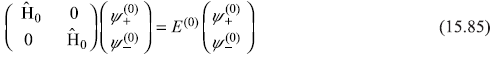
Or

and

The energy E⁽⁰⁾ simply represents the energy levels of unperturbed hydrogen atom

The wave functions are simply Pauli wave functions of electron with up and down spin states.

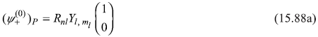
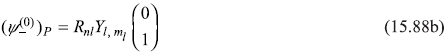
In the absence of spin–orbit interactions, both the above states have same energy. Therefore, any linear combination of these states is an eigenstate with same energy. We would like to form two mutually orthogonal states as linear combinations of these two states, in which the Hamiltonian is diagonal. Then all the operators represented in these new states, will be diagonal. Such new states may be formed by going from the uncoupled representation (where are well defined) to the coupled representation (where are well defined), that is, using the Clebsch–Gordon coefficients (discussed in Chapter 13). With the help of C–G coefficients given in Table 13.1, we may easily write Pauli wave functions in coupled representation (see Section 13.6):

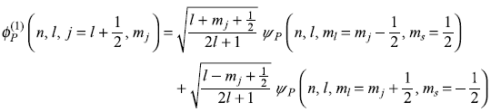
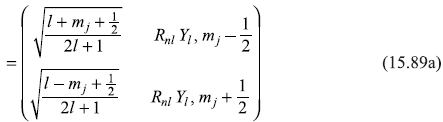
And a similar expression for the other Pauli wave function is

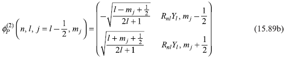
Now, as mentioned above, the states and are simultaneous eigenstates of operators and i.e.

and

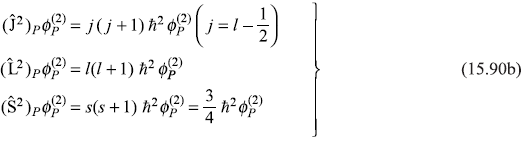
We have

so

Therefore, the first-order correction to energy due to spin–orbit interaction is given by

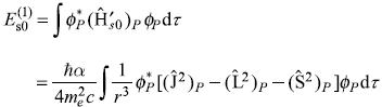
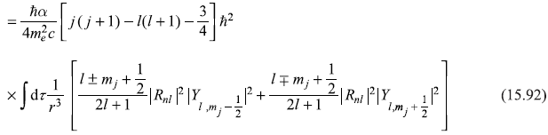
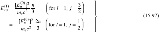
Here, one may note, the upper sign corresponds to the case j = [l + (1/2)] and the lower sign for j = [l – (l/2)].

The integration over angles may be easily carried out and we get,

or

and

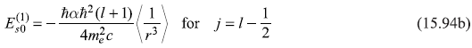
where

Therefore,

and

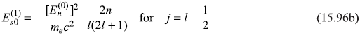
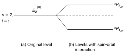
Figure 15.6 Fine structure due to spin–orbit interaction of ²P_1/2 and ²P_3/2 levels of hydrogen atom

For the particular case of l = 1, we get

In Figure 15.6, we show schematically the splitting of a level due to spin–orbit interaction.

15.7  THE ZEEMAN EFFECT

It was firstly observed by Zeeman that when atoms radiate in presence of a magnetic field, their individual spectral lines split into many lines. The phenomenon came to be known as Zeeman effect. As we shall see the phenomenon is a clear confirmation of vector atom model and space quantization. Firstly we shall discuss the so-called Normal Zeeman effect, where a single spectral line splits into three lines in presence of a magnetic field. In the next section, we shall discuss the anomalous Zeeman effect, where a single spectral line splits into more than three lines.

15.7.1  Normal Zeeman Effect

We shall study the changes in energy levels of a hydrogen-like atom when it is put in a constant homogeneous magnetic field. Let the magnetic field be in z-direction.

 

 

In the normal Zeeman effect, we ignore the effect of spin magnetic moment and consider only the interaction of orbital magnetic moment with the magnetic field. Obviously, the results obtained should be applicable to the cases where total spin of the atom is zero. In the next section, we shall include the interaction of spin magnetic moment (also) with the magnetic field.

Let the orbital magnetic moment of the atom be μ₁. The total Hamiltonian of the atom in presence of field B is given as

 

 

where

and

Ĥ may be re-written as

The Hamiltonian Ĥ₀ has eigenvalue equation

Now as commutes with Ĥ₀ (Chapter 10), so and Ĥ₀ have simultaneous eigenstates. Therefore, Schrodinger equation in presence of magnetic field B is

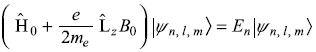
which gives

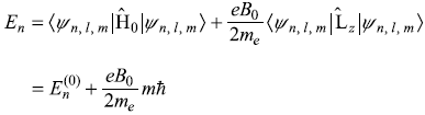
The (2l + 1) fold degenerate states which have energy in absence of B, have (2l + 1) (equi-spaced) different energies E_n in presence of B. The frequencies of the spectral lines emitted in transitions between two different states of the atom are given by

or

where ∆m = m₂ – m₁ is the change of the magnetic quantum number m in the transitions. We know from selection rules (discussed in Chapter 17) that

 

 

and also that the light emitted in the transitions for which ∆m = 0, is polarized parallel to B while in transitions for which ∆m = ±1, the polarization is perpendicular to B. Thus, we get

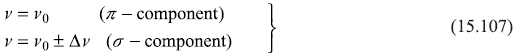
Figure 15.7 Normal Zeeman effect: Energy level corresponding to l = 2 splits into five and that corresponding to l = 1 splits into three levels. Because of the selection rule ∆m_l = 1,0 –1, there are three spectral lines of energies (h v₀ + µ_BB), h v₀, and (h v₀ – µ_BB)

where ∆v = (µ_BB₀/h). We show in Figure 15.7 the schematic diagram of the possible transitions between levels with l₂ = 2 and l₁ = 1.

15.7.2  Anomalous Zeeman Effect

When a hydrogen-like atom is put in a constant homogeneous magnetic field and the atom has non-zero spin angular momentum, the Hamiltonian may be written as

Where

Here represents the spin-orbit interaction and Ĥ″ represents the interaction of atom with magnetic field B. We shall assume the field B to be weak such that the effect of interaction Ĥ″ is smaller than that of spin-orbit interaction. So, we shall consider the eigenstates of as basis states and shall treat Ĥ″ as a small perturbation.

In Section 15.6, we found the Pauli wave functions [given by Eqs (15.89a) and (15.89b)] corresponding to j = [l + (1/2)] and j = [l – (1/2)], respectively, which work as basis states in presence of spin-orbit interaction . We found there that as a result of , the energy levels split and each level is characterized by well-defined values of J², L², and S². We shall use these basis states of Eqs (15.89a) and (15.89b) to find the contribution of perturbation Ĥ″.

We may write the Pauli operator for Ĥ″ as

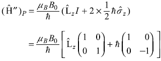
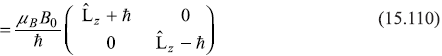
Now, as we know

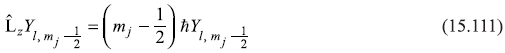
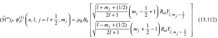
we may operate (Ĥ″)_P on basis state [given by Eq. (15.89a)] to get

and

and similarly we get

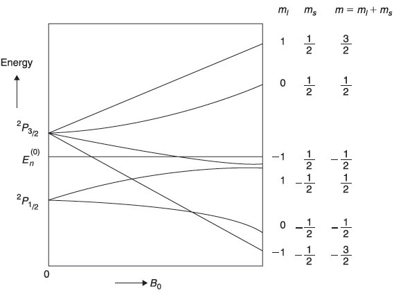
Figure 15.8 Schematic plot of the splitting of ²P energy level by magnetic field. The two levels corresponding to B₀ = 0 represent the spin-orbit splitting

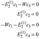
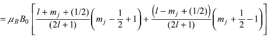
Let us consider the splitting of P-state (l = 1) of, say, an alkali atom. For l = 1, we have j = (3/2) and (1/2). So, we get

In Figure 15.8, we show schematically the splitting of ²P energy level by magnetic field.

EXERCISES

Exercise 15.1

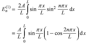
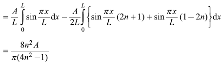
Consider a particle in a one-dimensional potential box with walls at x = 0 and x = L. Find the first-order correction to and due to the following perturbations:

•  
  V′(x) = Ax
•  
  V′(x) = Ax²
•  
  
•  
  

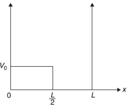
Figure 15.9 The potential raised by V₀ in half the well

Exercise 15.2

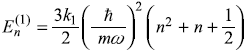
A linear harmonic oscillator is perturbed by the potential

 

 

Find the first-order correction to energy .

Exercise 15.3

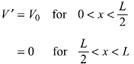
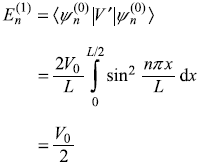
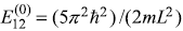
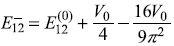
Consider a particle in a one-dimensional potential box with its walls at x = 0 and x = L, the system is perturbed such that the potential now is [see Figure (15.9)]

• Calculate the first-order correction to energy eigenvalues.
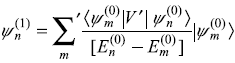
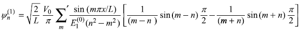
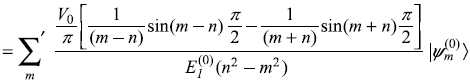
• Find the first-order correction to eigenstates.
• If the particle is an electron and it makes transitions, how do the frequencies emitted by the perturbed system compare with those of the unperturbed system?
• Up to what value of V₀ are the perturbation theory results valid?

Exercise 15.4

A two-level unperturbed system is described by the Hamiltonian . Now a small perturbation is switched on, which may be represented by

• Find the first-order correction to energy eigenvalues.
• Find the second-order correction to eigenvalues.
• Compare the eigenvalues including up to second-order corrections with the exact eigenvalues of Ĥ(= Ĥ₀ + V′).
• Find eigenstates up to first-order correction.

Exercise 15.5

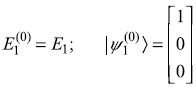
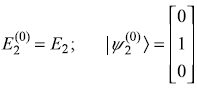
The Hamiltonian of a three-level system is given as .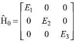

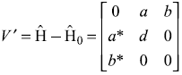
After a small perturbation, its Hamiltonian is given as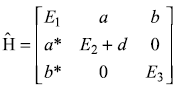

• find the first-order corrections to energy eigenvalues.
• Find the second-order corrections to eigenvalues.
• Find out the first-order correction to eigenstates.

Exercise 15.6

A hydrogen atom in its ground state is put in a constant homogeneous electric field pointing in z-direction, so the interaction energy is H′ = eE₀ r cosθ. Show that there is no change in the ground state energy of the atom up to first-order in the electric field.

Exercise 15.7

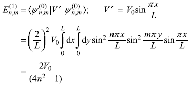
Consider a particle in a two-dimensional square potential well of side L.

 

 

Now a perturbation V′ is introduced such that

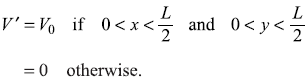
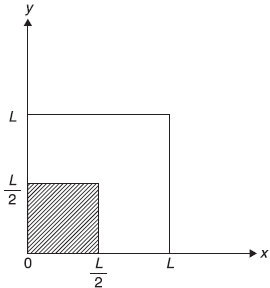
Figure 15.10 Two-dimensional potential well with (1/4)th part (shaded region) having potential raised by constant amount V₀

This raises the potential in one quarter of the well by an amount V₀ [see Figure (15.10)].

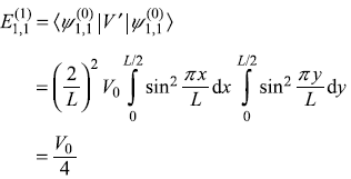
• Find the first-order correction to the ground state energy.
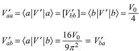
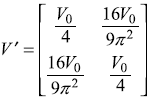
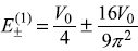
• Find the first-order correction to the first excited state energy.

Exercise 15.8

In Exercise 15.7, the particle in the two-dimensional square potential well, is perturbed by the potential V′ = V₀ sin(πx/L). Find first-order correction to the energy of state.

Exercise 15.9

When a hydrogen atom is put in a constant homogeneous electric field (in z-direction) the four-fold degeneracy of n = 2 states is partially lifted (the Stark effect). Estimate the electric dipole moment of hydrogen atom in the state.

•  
  
•  
  

Exercise 15.10

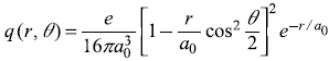
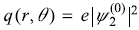
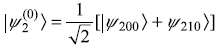
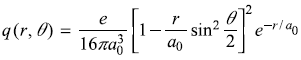
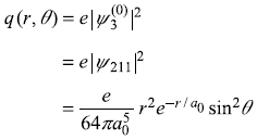
In Exercise 15.9, what is the electron charge density q(r, θ) associated with the state

•  
  
•  
  
•  
  
•  
  

Exercise 15.11

In a magnetic field of 2.0 T, the Zeeman components of a 550 nm spectral line are 0.028 nm apart. From these data find the ratio (e/m_e).

Exercise 15.12

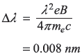
An atomic gas it put in a magnetic field of 0.5 T. When suitably excited the atoms give spectral lines with Zeeman components. How far apart are the Zeeman components of the 590 nm spectral line?

SOLUTIONS

Solution 15.1

•  
  
  
•  
  
•  
  
  

Solution 15.2

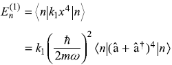
Only those terms contribute which have equal number of creation and annihilation operators. We get

Solution 15.3

•  
  
• The first-order correction to nth eigenstate is
  
  

  or

  
• As first-order correction to eigenvalue is same for all states, the emitted frequencies remain unchanged.
• The results of perturbation theory are valid only for .

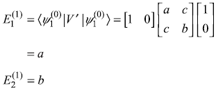
Solution 15.4

The unperturbed eigenvalues (of Ĥ₀) are

with corresponding eigenstate

with corresponding eigenstate

• First-order correction to eigenvalue
  
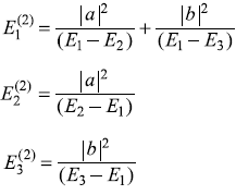
• Second-order corrections
  
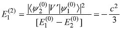
• So up to second-order, the energy levels are
  

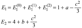
  Exact eigenvalues of Ĥ are

  

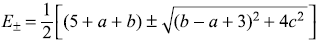
  We may have binomial expansion for small values of c. Then

  

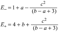
  which give same values as E₁ and E₂ above, for small values of a and b.

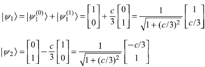
• First-order corrections to eigenstates:
  

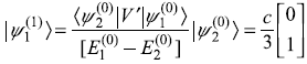
  and, similarly

  

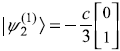
  Therefore, normalized eigenstates including first-order correction are

  

Solution 15.5

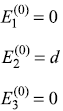
The unperturbed eigenvalues and eigenstates are

Perturbation Hamiltonian V′ is

• First-order correction to eigenvalues:
  
• Second-order corrections:
  
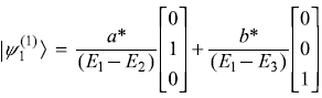
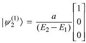
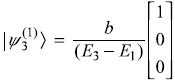
• First-order correction to eigenstates:
  
  
  

Solution 15.6

First-order correction to ground state energy of hydrogen atom

may be easily shown to vanish.

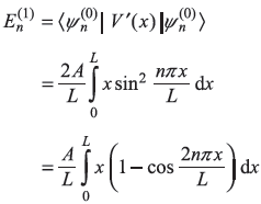
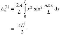
Solution 15.7

Unperturbed energy eigenvalues and eigenstates are

•  
  
• The first excited states (let us call it ) and (call it) are doubly degenerate. Let us firstly construct the 2 × 2 matrix of the total Hamiltonian in these basis states.
  

  Therefore,

  

  Using the results of doubly-degenerate perturbation theory, the changes in energy are given as Eq. (15.51)

  

  So the energy of first excited state, which was before perturbation, splits into two energies

  

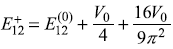
  and

  

Solution 15.8

Solution 15.9

The interaction energy between an electric dipole moment D and the electric field E is [see Eq. (15.58)],

 

• We had found that eigenvalue of H′ in state
  

  so

  –D · E = 3|e|a₀E

  and

  D = –3|e|a₀e_z

  (i.e., dipole moment is in opposite direction to electric field),

• In state the eigenvalue of H′ is –3|e|α₀Ε

  So

   

  D = 3|e|a₀e_z

  (i.e., dipole moment is in the direction of electric field).

Solution 15.10

•  
  

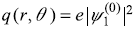
  where

  

  so

  
•  
  
  

  and

  
•  
  
• same expression as above.

Solution 15.11

The separation of Zeeman components is

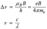
so

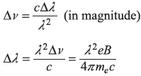
or

Solution 15.12

REFERENCES

1. Levi, A.F.J. 2003. Applied Quantum Mechanics. Cambridge, MA.: Cambridge University Press.
2. Matthews, P.T. 1974. Introduction to Quantum Mechanics, 3rd edn., London, UK: McGraw-Hill.
3. Baym, G. 1969. Lectures on Quantum Mechanics. Massachusetts: Benjamin/Cummings.