
Chapter 11
Angular Momentum–Revisited
11.1 INTRODUCTION
In Chapter 9, we studied orbital angular momentum. There, we defined orbital angular momentum operators ![]() and components
and components ![]() We found out their commutation relations and found simultaneous eigenfunctions and eigenvalues of
We found out their commutation relations and found simultaneous eigenfunctions and eigenvalues of ![]() Let us rewrite some of these relations.
Let us rewrite some of these relations.
Here we have written the eigenstates Yl, m(θ, ϕ) in the ket notation as ![]() In this chapter, we shall define raising and lowering operators. Using properties of these operators, we shall find out, in a very simple way, the eigenvalues and eigenstates of angular momentum operators. We shall also express angular momentum operators in matrix form.
In this chapter, we shall define raising and lowering operators. Using properties of these operators, we shall find out, in a very simple way, the eigenvalues and eigenstates of angular momentum operators. We shall also express angular momentum operators in matrix form.
11.2 RAISING AND LOWERING OPERATORS (THE LADDER OPERATORS)
In Chapter 9, we found eigenvalues and eigenstates of operators ![]() and
and ![]() by solving the corresponding Schrodinger equations (in the form of second/first order differential equations). In this chapter, we use an alternative method to arrive at same results of eigenvalues and eigenstates of these operators. This method is simpler and straight forward. The method uses the so-called raising and lowering operators (or the ladder operators) which we shall define below.
by solving the corresponding Schrodinger equations (in the form of second/first order differential equations). In this chapter, we use an alternative method to arrive at same results of eigenvalues and eigenstates of these operators. This method is simpler and straight forward. The method uses the so-called raising and lowering operators (or the ladder operators) which we shall define below.
There are two classes of angular momenta: the orbital angular momentum (denoted by L) and the spin angular momentum (denoted by S). We start denoting the angular momentum, in general, by J. So J may represent L or S or the combination L + S. We define the commutation relations amongst the components of ![]() (similar to those in components of
(similar to those in components of ![]() ), as
), as
The raising and lowering operators ![]() and
and ![]() are defined as
are defined as
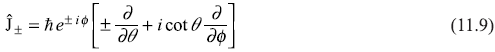
Using Eqs (9.18b) and (9.18c), we may write these operators as
Now, one may easily see that
Similarly,
Also, we have
Other relations that ![]() and
and ![]() satisfy are
satisfy are
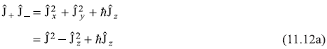
From Eqs (11.12), we may write
11.3 EIGENVALUES AND EIGENSTATES OF ORBITAL ANGULAR MOMENTUM OPERATORS: SECOND CONSTRUCTION OF SPHERICAL HARMONICS
Let us now turn to finding eigenvalues and eigenstates of operators ![]() and
and ![]() We start with eigenvalue equation of operator Jz,
We start with eigenvalue equation of operator Jz,
where we have to find eigenvalues mħ and eigenstates φm(ϕ). We now consider the operation
This equation implies that ![]() is an (unnormalized) eigenstate of
is an (unnormalized) eigenstate of ![]() corresponding to eigenvalue (m + 1)ħ . That simply means
corresponding to eigenvalue (m + 1)ħ . That simply means
where C+(m) is some constant (to be determined later) and for the time being we replace it by unity. So in the place of Eq. (11.17), we write
Now applying J+ on φm +1, we get
Similarly, we get
But we shall take constant C–(m) to be unity, so
and
Here we observe that operation of J+ on an eigenstate φm of ![]() generates another eigenstate φm+1 of
generates another eigenstate φm+1 of ![]() . The successive operations of
. The successive operations of ![]() generate eigenstates φm+2, φm+3 ... and so on. Therefore, we have found a scheme of generating a sequence of eigenstates of operator
generate eigenstates φm+2, φm+3 ... and so on. Therefore, we have found a scheme of generating a sequence of eigenstates of operator ![]() starting from the eigenstate φm: the successive eigenstates have values of m in the sequence differing by unity,
starting from the eigenstate φm: the successive eigenstates have values of m in the sequence differing by unity,
The corresponding eigenvalues of operator ![]() in these eigenstates being respectively
in these eigenstates being respectively
As the operators ![]() and
and ![]() commute, these two have common eigenstates. Let φm be the common eigenstate with eigenvalue K2 ħ2 of operator
commute, these two have common eigenstates. Let φm be the common eigenstate with eigenvalue K2 ħ2 of operator ![]() . So
. So
where we have to determine values of K2. Now, we know that operators ![]() and
and ![]() commute [(Eq. (11.11)], so
commute [(Eq. (11.11)], so
or
Equation (11.23) dictates that ![]() is an eigenstate of
is an eigenstate of ![]() corresponding to eigenvalue K2 ħ2. Therefore, all eigenstates of
corresponding to eigenvalue K2 ħ2. Therefore, all eigenstates of ![]() found in Eq. (11.15) are the eigenstates of
found in Eq. (11.15) are the eigenstates of ![]() corresponding to the same eigenvalue K2 ħ2. Let us firstly see how many such eigenstates are there:
corresponding to the same eigenvalue K2 ħ2. Let us firstly see how many such eigenstates are there:
From Eqs (11.15) and (11.22), the expectation values of ![]() and
and ![]() in state φm are
in state φm are
But we also have
Therefore,
As ![]() and
and ![]() it follows from Eq. (11.25) that
it follows from Eq. (11.25) that
or
It may be noted that for a given value of K (> 0), Eq. (11.27) dictates that the possible values of m in Eq. (11.21) must lie in between +K and –K. Therefore, if the maximum possible value of m, for a given value Kħ of the magnitude of angular momentum vector, is m+, then we should have the condition
Similarly, if m– is the minimum value of m for the angular momentum magnitude Kħ, we have
Now let the L.H.S. and R.H.S. operators of Eq. (11.12b) operate on state φm+, we get
or
or
Again with operators of Eq. (11.12a) operating on state φm–, we get
or
or
From Eqs (11.29) it follows that
Apart from the trivial solution m+ = m–= 0, this equation is satisfied if
Hence, for a given magnitude K2 ħ2 of J2, the allowed values of m are like the following sequence (see Figure 11.1).
where m+ (the maximum value of m) and m– (the minimum value of m) are given by Eqs (11.29a) and (11.29b), respectively. Thus all possible values of m form a symmetric sequence about m = 0. The successive values of m differ by unity. Let us call maximum value of m as j.
Therefore, m runs from –j to +j in unit steps. Clearly, one of the two possibilities is there:
-
If m = 0 is present in the sequence of m values, then
j = an integer (11.34a) -
If m = 0 is not present in the sequence of m values, then

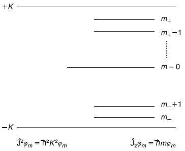
Figure 11.1 For a given eigenvalue of ![]() , the allowed values of m are shown. Successive values of m differ by unity
, the allowed values of m are shown. Successive values of m differ by unity
In fact, it can be easily seen that if we take any other choice of j [other than those of Eqs (11.34a) and (11.34b)], then all possible values of m shall not satisfy the conditions which the sequence of m should satisfy, which we state again: The possible values of m should form a symmetric sequence about m = 0 and the successive values of m should differ by unity.
Let us take some particular examples.
- If j is an integer say 3, the corresponding m values are 3, 2, 1, 0, –1, –2, –3.
- If j is an odd multiple of
 say
say  the corresponding m values are
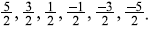
- If we take j different than those of category (i) and (ii) above, say
 the corresponding m values should be
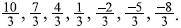
It is clearly seen that the choice of j in category (iii) does not give m values that satisfy the above mentioned criterion for the sequence of m values.
In fact, in either case of category (i) and (ii), for a given value of j, the allowed values of m run from –j to +j (see Figure 11.2), so inserting j = m+ = – m– into Eq. (11.29), we get the eigenvalues of J2 as
and eigenvalues of Jz as
where j is an integer or half an odd integer. The eigenvalue equations of ![]() and
and ![]() are for general angular momentum
are for general angular momentum ![]() which could be orbital angular momentum
which could be orbital angular momentum ![]() spin angular momentum
spin angular momentum ![]() or their sum
or their sum ![]() In the following work, we consider
In the following work, we consider ![]() representing orbital angular momentum
representing orbital angular momentum ![]() , where corresponding quantum numbers l and m1 (we start writing now l and m1 for j and mj) have integral values. In a later section, we shall consider
, where corresponding quantum numbers l and m1 (we start writing now l and m1 for j and mj) have integral values. In a later section, we shall consider ![]() representing
representing ![]() and then quantum numbers j and mj shall have half an odd integer values.
and then quantum numbers j and mj shall have half an odd integer values.
For orbital angular momentum ![]() Eqs (11.35) become
Eqs (11.35) become
and
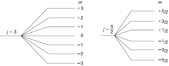
Figure 11.2 Allowed values of quantum number m for a given value of orbital quantum number j. j may be either an integer or an odd multiple of one-half
As per Eqs (11.15) and (11.22), the state φml is simultaneous eigenstate of ![]() and
and ![]() . These two operators have eigenvalues l (l + 1) ħ2 and m1 ħ, respectively, therefore, the eigenstate φml should really be assigned two quantum numbers l and ml and so we rewrite these eigenstates as φl,ml.
. These two operators have eigenvalues l (l + 1) ħ2 and m1 ħ, respectively, therefore, the eigenstate φml should really be assigned two quantum numbers l and ml and so we rewrite these eigenstates as φl,ml.
At this stage, we can borrow a simple result from Chapter 9. There we found the eigenstates of operator ![]() [(Eq. (9.22)].
[(Eq. (9.22)].
Now the simultaneous eigenstate φl,ml of ![]() and
and ![]() may be written as product of two functions
may be written as product of two functions
We shall simply write m in place of ml in what follows. Let us start now with Eq. (11.28a), which we rewrite as
(as maximum value of m is l)
or
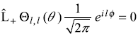
Using the expression of ![]() [Eq. (11.9)], the above equation gives
[Eq. (11.9)], the above equation gives
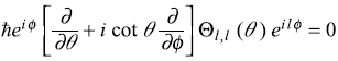
or
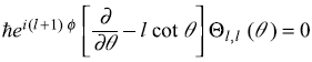
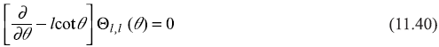
Solution of this equation is
The multiplicative normalization constant will be obtained later. Eq. (11.38) gives
Let us start calling the functions φl,m(θ, ϕ)(when normalized) as Yl,m(θ, ϕ).
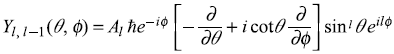
So, Eq. (11.42) is written as
where Al is the normalization constant. From Eq. (11.43) one may easily find expressions of Y0,0(θ, ϕ), Y1,1(θ, ϕ), Y2,2(θ, ϕ), Y3,3(θ, ϕ), ... which we write below
Here constants A0, A1, A2, ... are determined by normalizing the eigenstate. One notices that these expressions are same as the corresponding expressions of Y1, 1 (θ, ϕ) in Table 9.1 of Chapter 9.
Let us now apply the lowering operator ![]() on both sides of Eq. (11.43). We have
on both sides of Eq. (11.43). We have
or
where Bl is the normalization constant. From Eq. (11.45), we may write expressions of Y1,0(θ, ϕ), Y2,1(θ, ϕ), Y3,2(θ, ϕ) and so on, which are
which are same as those obtained in Chapter 9 and shown in Table 9.1.
Proceeding in a similar way one may easily find expressions of other spherical harmonics like
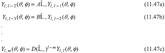
Here A, B, ... D are normalization constants.
11.4 THE CONSTANTS C+ AND C_
Let us recollect that constants C+ (m) and C–(m) were defined through the operation of raising and lowering operators ![]() and
and ![]() on eigenstate φm [Eqs (11.17) and (11.19)]. As discussed in the previous Section, the state φm is simultaneous eigenstate of
on eigenstate φm [Eqs (11.17) and (11.19)]. As discussed in the previous Section, the state φm is simultaneous eigenstate of ![]() and
and ![]() and, therefore, (state φm) should be assigned two quantum numbers j and m and should be rewritten as φj,m. Furthermore, this eigenstate φj,m can be expressed as the product of two functions Θj,m(θ) and Φm(ϕ) as
and, therefore, (state φm) should be assigned two quantum numbers j and m and should be rewritten as φj,m. Furthermore, this eigenstate φj,m can be expressed as the product of two functions Θj,m(θ) and Φm(ϕ) as
We now denote eigenstate φj,m(θ, ϕ) as eigenket ![]() and write various operator equations as
and write various operator equations as
Equations (11.17) and (11.19) showing operations of ![]() and
and ![]() are rewritten as
are rewritten as
Let us now determine coefficients C+ and C–. Taking adjoint of both sides of Eq. (11.50a), we get
(since ![]() is adjoint of
is adjoint of ![]() )
)
Now multiplying Eqs (11.50c) and (11.50a), we have
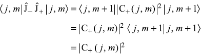
Putting value of ![]() from Eq. (11.12b) gives
from Eq. (11.12b) gives
Thus,
Similarly, we may get
It is clear from above expressions that
11.5 MATRIX REPRESENTATION OF ANGULAR MOMENTUM OPERATOR CORRESPONDING TO j = 1
We shall now proceed to represent the angular momentum operators ![]() and components
and components ![]() in matrix form in a basis in which operators
in matrix form in a basis in which operators ![]() and
and ![]() are diagonal. That simply means the simultaneous eigenkets of
are diagonal. That simply means the simultaneous eigenkets of ![]() and
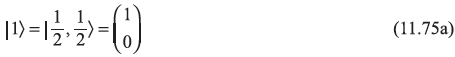
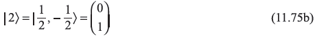
and ![]() are chosen as basis vectors. Let us take the case corresponding to angular momentum quantum number j = 1. For j = 1, the allowed values of m are 1, 0 and –1. So, there are three basis states, which we denote by
are chosen as basis vectors. Let us take the case corresponding to angular momentum quantum number j = 1. For j = 1, the allowed values of m are 1, 0 and –1. So, there are three basis states, which we denote by ![]() and
and ![]() and write as
and write as
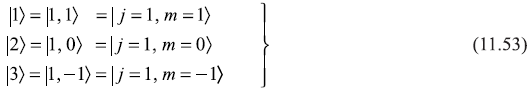
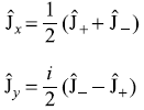
Using Eqs (11.49a) and (11.49b) we have
which in the notations of Eq. (11.53) are written as
Similarly,
In the basis set ![]() the (m, n)th matrix element of an operator  is defined as
the (m, n)th matrix element of an operator  is defined as
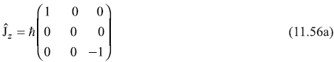
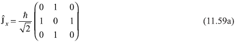
Therefore,
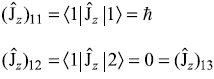
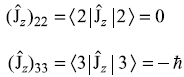
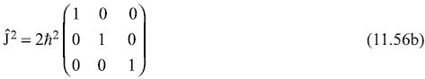
We find that, in fact, all off-diagonal terms are zero. So matrix form of ![]() may be written as
may be written as
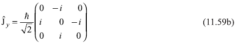
Similarly, we get
Therefore, the matrix form of ![]() is
is
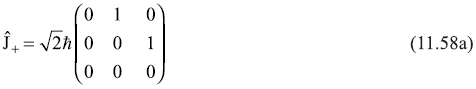
Now using Eqs (11.50a) and (11.51a), we get
So matrix form of ![]() is
is
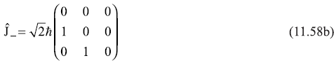
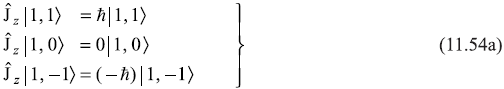
Now
Therefore, matrix forms of ![]() and
and ![]() are
are
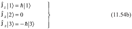
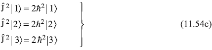
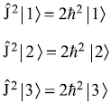
It is clear from the matrix form of ![]() [Eq. (11.56a)] that it has the following three eigenstates and eigenvalues:
[Eq. (11.56a)] that it has the following three eigenstates and eigenvalues:
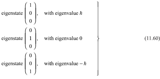
And same are the eigenstates of the matrix form of ![]() (with eigenvalues 2ħ2 for each state). Therefore, we may write eigenkets
(with eigenvalues 2ħ2 for each state). Therefore, we may write eigenkets ![]() in the (column) matrix form as
in the (column) matrix form as
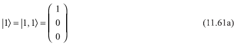
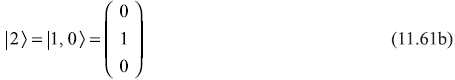
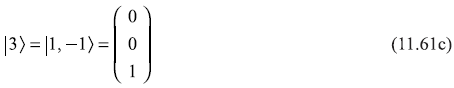
It may be easily checked that column matrices (or generally called column vectors) of Eq. (11.61) represent the correct eigenstates. For example, L.H.S. of Eq. (11.57b) gives
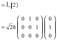
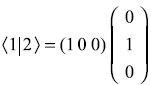
Also we may check, these column vectors are orthogonal to each other. For example
11.6 MATRIX REPRESENTATION OF ANGULAR MOMENTUM OPERATOR CORRESPONDING TO 
It is to be noted that the results obtained in this chapter and Chapter 9 are in connection with the orbital angular momentum operator ![]() Though in defining the raising and lowering operators, we had used the general angular momentum operator
Though in defining the raising and lowering operators, we had used the general angular momentum operator ![]() which may represent orbital angular momentum operator
which may represent orbital angular momentum operator ![]() or spin angular momentum operator
or spin angular momentum operator ![]() or their combination, that is,
or their combination, that is, ![]() Yet in Eq. (11.9), while writing the expressions for raising and lowering operators
Yet in Eq. (11.9), while writing the expressions for raising and lowering operators ![]() and
and ![]() we had used only x- and y- components of orbital angular momentum operator. Therefore, the results for the spectrum of magnetic quantum number m for a given quantum number j (i.e., m values lying symmetric about m = 0, ranging from –j to +j, differing by unity) should be applicable to the orbital angular momentum only. As we know the case of j = an integer corresponds to the orbital angular momentum. However, value of j = half an odd integer is also possible, as it allows m values lying symmetric about m = 0, ranging from –j to +j, differing by unity. Therefore, the values of
we had used only x- and y- components of orbital angular momentum operator. Therefore, the results for the spectrum of magnetic quantum number m for a given quantum number j (i.e., m values lying symmetric about m = 0, ranging from –j to +j, differing by unity) should be applicable to the orbital angular momentum only. As we know the case of j = an integer corresponds to the orbital angular momentum. However, value of j = half an odd integer is also possible, as it allows m values lying symmetric about m = 0, ranging from –j to +j, differing by unity. Therefore, the values of ![]() which are not there in case of orbital angular momentum operator, may be there corresponding to some other angular momentum operator. Let us consider the case of
which are not there in case of orbital angular momentum operator, may be there corresponding to some other angular momentum operator. Let us consider the case of ![]() and find out the matrix form of the corresponding angular momentum operator. We shall, in fact, see that the form of the resulting matrix operators is those of familiar Pauli spin matrices.
and find out the matrix form of the corresponding angular momentum operator. We shall, in fact, see that the form of the resulting matrix operators is those of familiar Pauli spin matrices.
So we proceed to represent operator ![]() and component operators
and component operators ![]() (in matrix form) corresponding to angular momentum quantum number
(in matrix form) corresponding to angular momentum quantum number ![]() in a basis in which
in a basis in which ![]() and
and ![]() are diagonal. Now corresponding to
are diagonal. Now corresponding to ![]() , the magnetic quantum number
, the magnetic quantum number ![]() and
and ![]() There are two basis states denoted by
There are two basis states denoted by ![]() and
and ![]() where
where
Using Eqs (11.49a) and (11.49b), we have
which may be rewritten as
Also, we have
We may easily find the matrix elements of ![]()
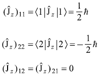
So matrix form of ![]() is
is
Similarly, using Eqs (11.65) we may find out various matrix elements of ![]() giving the resulting matrix of form
giving the resulting matrix of form
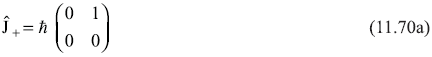
Now using Eq. (11,50a), we have
where ![]() is calculated using Eq. (11.51a)
is calculated using Eq. (11.51a)
So, Eq. (11.68) gives
And it can be easily seen that
The matrix form of ![]() is
is
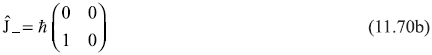
Similarly, ![]() is
is
From these equations, we find ![]() and
and ![]() as
as
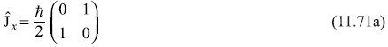
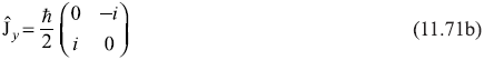
The angular momentum component operators ![]() given by matrices of Eqs (11.71a), (11.71b), and (11.66), respectively, may be expressed as
given by matrices of Eqs (11.71a), (11.71b), and (11.66), respectively, may be expressed as
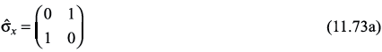
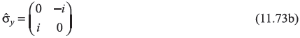
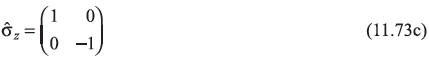
are known as the Pauli spin matrices.
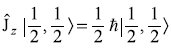
The 2 × 2 matrix representing ![]() has following two eigenstates and eigenvalues:
has following two eigenstates and eigenvalues:
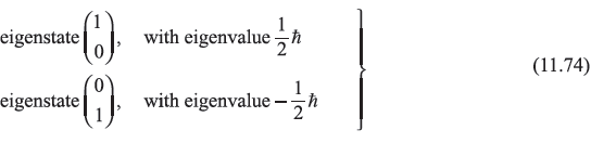
Therefore, the eigenkets ![]() and
and ![]() may be written in the column matrix form, generally termed as spinors:
may be written in the column matrix form, generally termed as spinors:
Any linear combination of column matrices will be a column matrix and, therefore, shall also be termed as spinor. Now, we have seen the angular momentum operator ![]() for quantum number
for quantum number ![]() has two eigenstates which represent two states of electron spin. Hence, we start writing
has two eigenstates which represent two states of electron spin. Hence, we start writing ![]() and
and ![]() in place of
in place of ![]() and
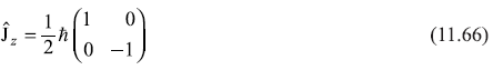
and ![]() and write quantum numbers s and ms in place of j and m. Therefore, Eq. (11.72) is rewritten for spin angular momentum operator
and write quantum numbers s and ms in place of j and m. Therefore, Eq. (11.72) is rewritten for spin angular momentum operator ![]()
EXERCISES
Exercise 11.1
Find the following expectation values in state ![]()


where
 represents the anti-commutator
Find out matrix form of following angular momentum operators, corresponding to quantum number ![]() in a basis in which
in a basis in which ![]() and
and ![]() are diagonal.
are diagonal.
Exercise 11.3
Consider a system of angular momentum with quantum number l = 1. Its angular momentum state is represented by state vector.
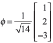
Find the probability that a measurement of Lz gives value 0.
SOLUTIONS
Solution 11.1
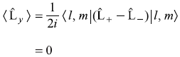
- First method: From Eq. (11.12a)
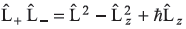
so
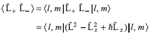 = l(l+1)ħ2 – m2ħ2 + ħ2m= ħ2[(l + m)(l – m + 1)] ( 11.77)
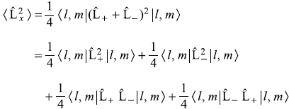
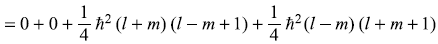
Second method:
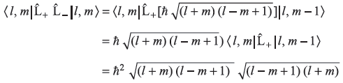 = ħ2[(l + m)(l – m+ 1)] (Refer to Eq. 11.77)
 -
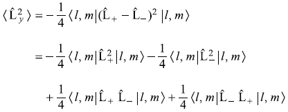
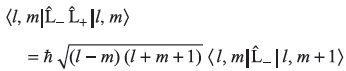 = ħ2[(l – m) (l + m + 1)] (11.78)
 -
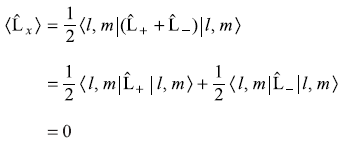
-
-

-

- From (a) and (b)
 = 2mħ2 (11.81)
 -
 = 2ħ2 [l(l + 1) – m2] (11.82)
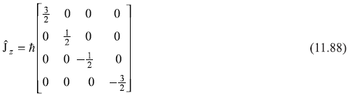
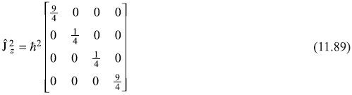
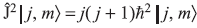
![]() are the simultaneous eigenkets of operators
are the simultaneous eigenkets of operators ![]() and
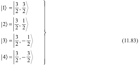
and ![]() For angular momentum quantum number
For angular momentum quantum number ![]() allowed values of m are
allowed values of m are ![]() So, there are four basis states, which we shall denote by
So, there are four basis states, which we shall denote by ![]() and
and ![]() written explicitly as
written explicitly as
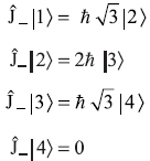
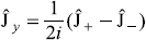
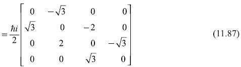
- Using Eqs (11.50a) and (11.51a), we have
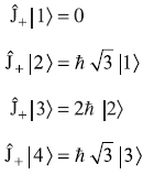
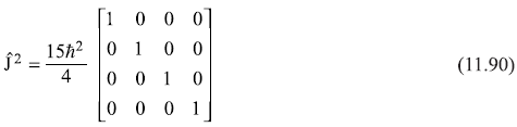
From these relations, one may find out all matrix elements
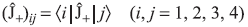
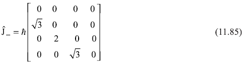
and may get matrix form of
 as
as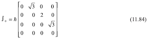
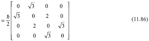
- Using Eqs (11.50b) and (11.51b), we have
-
-
-
-
- We know
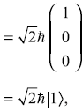
We know three basis state vectors of operator ![]() are
are  and
and ![]() corresponding to eigenvalues of
corresponding to eigenvalues of ![]() and –ħ, respectively. The state vector ϕ may be written as
and –ħ, respectively. The state vector ϕ may be written as
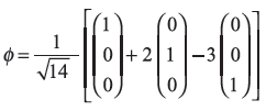
So the probability for ![]() to have eigenvalue 0 is
to have eigenvalue 0 is ![]()
REFERENCES
- Griffiths, D.J. 1995. Introduction to Quantum Mechanics. New York, NY: Prentice Hall.
- Tinkham, M. 1964. Group Theory and Quantum Mechanics. New York, NY: McGraw-Hill.
- Sakurai, J.J. 1985. Modern Quantum Mechanics. Massachusetts: Benjamin/Cummings.
- Liboff, R.L. 1992. Introductory Quantum Mechanics. Massachusetts: Addison-Wesley.
- Merzbacher, E. 1999. Quantum Mechanics. 3rd edn., New York, NY: John Wiley & Sons.