
Chapter 9
Angular Momentum
9.1 INTRODUCTION
It may be very well emphasized that the study of the application of quantum mechanics to three-dimensional systems, almost invariably, involves the description of the properties of angular momentum. For example, in connection with the quantum mechanical study of (i) states of electrons in atoms and molecules and (ii) states of nucleons (neutrons and protons) in the nuclei, the role of angular momentum is of paramount importance. Keeping these three-dimensional systems in mind, we firstly discuss orbital angular momentum in this chapter and shall take up the study of the solution of Schrodinger equation in three-dimensional potential in the next chapter.
In fact, the orbital angular momentum in quantum mechanics is intimately akin to the angular momentum in classical mechanics. However, in quantum mechanics, the concept of angular momentum is much more general than in classical mechanics. In quantum mechanics, the orbital angular momentum is defined exactly the same way as in classical mechanics, viz., L = r × p. We may, however, notice here that L is no more an ordinary vector, but is a vector operator (as p, appearing in the definition of L, is itself a vector operator). Moreover, in quantum mechanics, in addition to the orbital angular momentum, we also encounter the spin angular momentum. In contrast to orbital angular momentum, the spin angular momentum is an intrinsic (or internal) property of the elementary particles, such as electrons, protons, neutrons, and so on. And, in fact, spin angular momentum has no classical counterpart. We shall discuss the orbital angular momentum in this chapter, whereas the spin angular momentum shall be discussed in Chapter 12.
9.2 ORBITAL ANGULAR MOMENTUM OPERATOR
Let us consider a particle of mass m moving with velocity v. Its position vector is denoted by r and the linear momentum vector by p. In classical mechanics, the orbital angular momentum about the origin of the coordinate system, is defined as
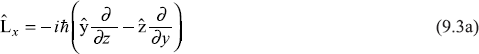
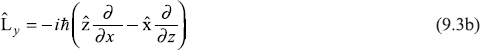
The vector L points in a direction perpendicular to the plane containing vectors r and p and has magnitude L = rmvsin θ (θ is the angle between r and p). The components of L in Cartesian coordinate system are
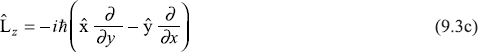
In quantum mechanics, we have the same definition of angular momentum L (and of its components Lx, Ly, Lz) as given above, but now x, y, z and px, py, pz are replaced by the corresponding operators {obeying commutation relations [Eq. (4.51)]}. So components Lx, Ly, Lz are now operators, given by
So, in terms of the three-dimensional linear momentum operator ![]() ,
,
the angular momentum operator L
is written as
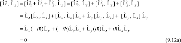
9.3 COMMUTATION RELATIONS
Using the basic commutation relations of Eq. (4.75), we can easily obtain the commutation relations obeyed by the operators ![]() and
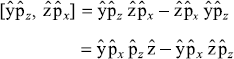
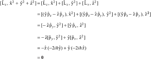
and ![]() As an example,
As an example,
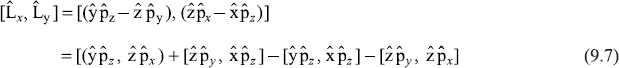
The first commutator on R.H.S of the above equation is
(as ![]() and
and ![]() commute with each other and with
commute with each other and with ![]() and
and ![]() )
)
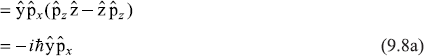
Similarly, the second commutator is
It can be easily seen that the rest two commutators in Eq. (9.7) vanish. Thus we get
Similarly, we may get
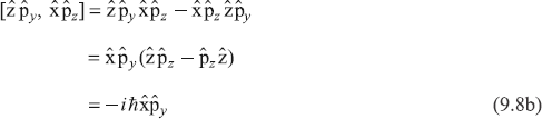
These three equations may be combined in a single equation
which in determinantal form, may be written as
It is quite evident that if ![]() were an ordinary vector, the vector product
were an ordinary vector, the vector product ![]() ×
× ![]() would vanish. But
would vanish. But ![]() is having the operator character and, therefore,
is having the operator character and, therefore, ![]() ×
× ![]() does not vanish. Equations (9.9) show none of the three (angular momentum) component operators
does not vanish. Equations (9.9) show none of the three (angular momentum) component operators ![]() commutes with any other. As mentioned in Chapter 4, when two operators do not commute, the corresponding observables are not simultaneously measurable. Therefore, it is not possible to assign simultaneously precise values to all the three or even any two components of the orbital angular momentum. As discussed earlier in Chapter 4 in connection with general operators, in the present context, if the system is in an eigenstate of one component operator (say
commutes with any other. As mentioned in Chapter 4, when two operators do not commute, the corresponding observables are not simultaneously measurable. Therefore, it is not possible to assign simultaneously precise values to all the three or even any two components of the orbital angular momentum. As discussed earlier in Chapter 4 in connection with general operators, in the present context, if the system is in an eigenstate of one component operator (say ![]() ), then a measurement of x-component of orbital angular momentum shall give a definite value. The other two components of angular momentum are, then, totally undermined. We shall discuss more about this in Section 9.6.
), then a measurement of x-component of orbital angular momentum shall give a definite value. The other two components of angular momentum are, then, totally undermined. We shall discuss more about this in Section 9.6.
Now from the form of orbital angular momentum operator
we may get form of operator ![]()
where the square of an operator is defined like
Let us calculate the commutator ![]()
Similarly, we may get
So, in general
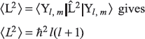
Therefore, the commuting operators ![]() and (say)
and (say) ![]() can have simultaneously the same eigenstate and, therefore, the values of magnitude of angular momentum and that of z-component of angular momentum may be determined precisely simultaneously.
can have simultaneously the same eigenstate and, therefore, the values of magnitude of angular momentum and that of z-component of angular momentum may be determined precisely simultaneously.
9.4 ANGULAR MOMENTUM OPERATOR IN SPHERICAL POLAR COORDINATES
We shall see that it is very convenient to find eigenstates and eigenvalues of operators ![]() and
and ![]() when one works in spherical polar coordinates (r, θ, ϕ) (shown in Figure 9.1). The polar coordinates (r, θ, ϕ) are related to the Cartesian coordinates (x, y, z) through the transformation equations
when one works in spherical polar coordinates (r, θ, ϕ) (shown in Figure 9.1). The polar coordinates (r, θ, ϕ) are related to the Cartesian coordinates (x, y, z) through the transformation equations
Also
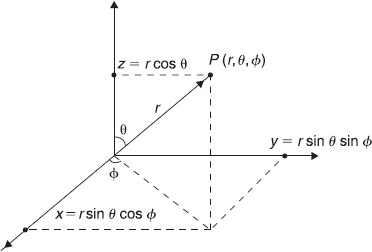
Figure 9.1 Spherical polar coordinates (r, θ, ϕ) of a point P.
From Eq. (9.13), we have
when solved, the above equations give
With the help of these equations, we may write
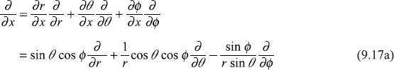
Similarly
and
Similarly, we may easily get
After a lengthy but straightforward algebra, we obtain
9.5 THE EIGENVALUES AND EIGENFUNCTONS OF  AND
AND 
We have seen in Section 9.3 that any two components of angular momentum operator ![]() do not commute and, therefore, the two components can not be known simultaneously. However, as seen in Section 9.3, the operator
do not commute and, therefore, the two components can not be known simultaneously. However, as seen in Section 9.3, the operator ![]() commutes with any component of
commutes with any component of ![]() . Therefore, simultaneous eigenfunctions of
. Therefore, simultaneous eigenfunctions of ![]() and of one of its components (say
and of one of its components (say ![]() ) may be found. It further means that the magnitude of angular momentum and that of its z-component may be known simultaneously.
) may be found. It further means that the magnitude of angular momentum and that of its z-component may be known simultaneously.
In this section, we proceed to find simultaneous eigenfunctions of ![]() and
and ![]() . Let us firstly find eigenvalues and eigenfunctions of the operator
. Let us firstly find eigenvalues and eigenfunctions of the operator ![]() . Denoting the eigenvalues of
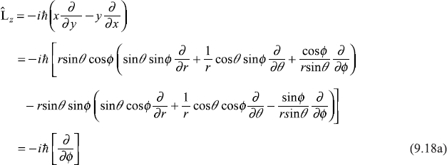
. Denoting the eigenvalues of ![]() by m ħ, and the corresponding eigenfunctions by Φm(ϕ), we have
by m ħ, and the corresponding eigenfunctions by Φm(ϕ), we have
Using (9.18a), we get
Equation (9.21) has the solutions
For the wave function to be single valued, the requirement is
or
which gives
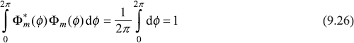
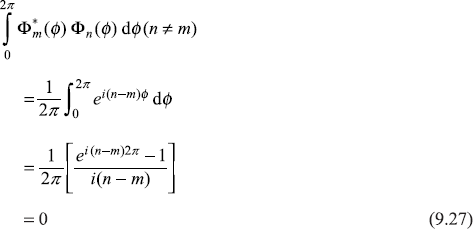
Hence the eigenvalues of ![]() are equal to mħ, where m = 0, ±1, ±2,.... So, if we have a measurement of z-component of the orbital angular momentum, it will give values 0, ±ħ, ±2ħ, ... . Now, the z-axis may be chosen along any arbitrary direction, we conclude that the component of orbital angular momentum along any axis is quantized and has values 0, ±ħ, ±2ħ, .... The quantum number m is known as the azimuthal or the magnetic quantum number. It can be easily checked that the eigen-functions Φm(ϕ) are orthonormal over the range 0 ≤ ϕ ≤ 2π.
are equal to mħ, where m = 0, ±1, ±2,.... So, if we have a measurement of z-component of the orbital angular momentum, it will give values 0, ±ħ, ±2ħ, ... . Now, the z-axis may be chosen along any arbitrary direction, we conclude that the component of orbital angular momentum along any axis is quantized and has values 0, ±ħ, ±2ħ, .... The quantum number m is known as the azimuthal or the magnetic quantum number. It can be easily checked that the eigen-functions Φm(ϕ) are orthonormal over the range 0 ≤ ϕ ≤ 2π.
and
Let us turn to find eigenvalues and eigenfunctions of operator ![]() , that is, to solve the eigenvalue equation
, that is, to solve the eigenvalue equation
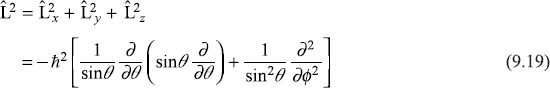
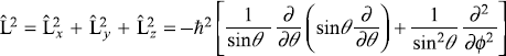
where λħ2 represents the eigenvalues of ![]() and Y (θ, ϕ) the corresponding eigenfunctions. Using the expression [Eq. (9.19)] of
and Y (θ, ϕ) the corresponding eigenfunctions. Using the expression [Eq. (9.19)] of ![]() in spherical polar coordinates, we have
in spherical polar coordinates, we have
Let us use the method of separation of variables and write
Substituting Eq. (9.30) in Eq. (9.29) and re-arranging the terms, we get

Expression on L.H.S. is a function of θ only, whereas that on R.H.S. is a function of variable ϕ only. So Eq. (9.31) shall hold only if each side is equal to a constant. Let this constant be m2. Therefore, we get the following two equations: one in variable θ, which is

and another in variable ϕ, which is
Equation (9.33) has the solution
Just like in Eqs (9.22) to (9.25), for the normalization of wave function Φ(ϕ), we get ![]() and for the wave function to be single valued we get m = 0, ±1, ±2, ... Therefore,
and for the wave function to be single valued we get m = 0, ±1, ±2, ... Therefore,
where
Now by a change of variables
Equation (9.32) becomes

The case m = 0
Let us consider the case m = 0, when Eq. (9.36a) reduces to
which is the well-known Legendre differential equation. It can be easily seen here that Eq. (9.36b) does not change its form when –µ is substituted for µ. So the solutions of Eq. (9.36b) are either even or odd functions of µ. The solution of Eq. (9.36b) may be written in the form of a series in powers of µ:
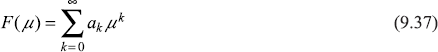
Differentiating Eq. (9.37) term by term, we have

and

Substituting Eqs (9.37), (9.38a), and (9.38b) in Eq. (9.36b), we get
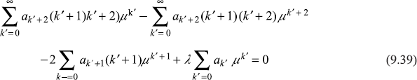
The above equation should be valid for all values of µ, therefore, the coefficients of each power of µ should be equated to zero. We collect the coefficient of µk and equate it to zero to get the recursion relation.
or
It may be noted from Eq. (9.40) that for the even solution (a1 = 0) all coefficients are proportional to a0, whereas for the odd solution (a0 = 0) all coefficients are proportional to a1. Now λħ2 denotes the eigenvalue of operator ![]() (which, being square of
(which, being square of ![]() , is a positive operator), so λ must be a non-negative number. We see from Eq. (9.40) that if the power series does not terminate at some fixed value of k, then for large k the ratio (ak+2/ak) ≈ [k/(k + 2)] ≈ 1. This behaviour suggests that the series [Eq. (9.37)] diverges logarithmically for µ = ±1. We conclude, therefore, that the power series should terminate at some finite value (say) k = l, where l is a non-negative integer. According to Eq. (9.40), series will terminate for k = l if λ has the value
, is a positive operator), so λ must be a non-negative number. We see from Eq. (9.40) that if the power series does not terminate at some fixed value of k, then for large k the ratio (ak+2/ak) ≈ [k/(k + 2)] ≈ 1. This behaviour suggests that the series [Eq. (9.37)] diverges logarithmically for µ = ±1. We conclude, therefore, that the power series should terminate at some finite value (say) k = l, where l is a non-negative integer. According to Eq. (9.40), series will terminate for k = l if λ has the value
where l is called as orbital angular momentum quantum number and has the values 0, 1, 2, 3, ... Thus, the eigenvalues of operator ![]() are l(l + 1)ħ2.
are l(l + 1)ħ2.
For l = 0, the series Eq. (9.37) has only one term with k = 0,
For l = 1, the series has two terms with k = 0, 1
For l = 2, the series has three terms with k = 0, 1, 2,
For l = 3, the series has four terms with k = 0, 1, 2, 3
and so on.
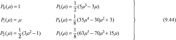
The resulting polynomials are known as Legendre polynomials Pl(µ), so, now we start writing F(µ) as P1(µ). It is clear that these are uniquely defined, apart from an arbitrary multiplicative constant. By convention, this constant is chosen such that
Also, since the Legendre polynomial Pl(µ) is either in even or odd powers of µ, depending on whether l is even or odd, we have
The first few Legendre polynomials evaluated, using Eqs (9.37) and (9.40), are
The Legendre polynomials may be expressed in the concise form, called the formula of Rodrigues;
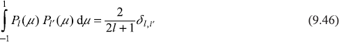
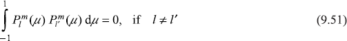
The Legendre polynomials satisfy orthogonality relations
and follow the recurrence relations
So, we have found the orthonormal sets of solutions of Eq. (9.36b) [and of Eq. (9.36a)] for m = 0 and using the relations of Eqs (9.30) and (9.34), the solutions may be written as
and
The General Case
Now after solving Eq. (9.36b) which is really Eq. (9.36a) with m = 0, the solution to Eq. (9.36a) may be obtained as follows:
Let us construct the so called associated Legendre functions ![]() by differential operations on Legendre function Pl(µ).
by differential operations on Legendre function Pl(µ).
(for positive integers m ≤ l).
Then differentiating Legendre’s equation [Eq. (9.36b)] m times with λ = l(l + 1) and using the definition (9.49), after a bit lengthy but straight forward algebra, we obtain the equation

which is identical with Eq. (9.36a) for λ = l(l + 1). So associated Legendre functions ![]() with m ≤ l are the acceptable solutions of Eq. (9.36a). The associated Legendre functions are orthogonal
with m ≤ l are the acceptable solutions of Eq. (9.36a). The associated Legendre functions are orthogonal
Also, we note that
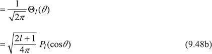
Now, the simultaneous eigenfunctions Yl, m(θ, ϕ) of both the operators ![]() and
and ![]() , which are normalized to unity on the unit sphere, are called spherical harmonics. Using Eqs (9.30), (9.22), and (9.52), we see that Yl, m(θ, ϕ) are given by
, which are normalized to unity on the unit sphere, are called spherical harmonics. Using Eqs (9.30), (9.22), and (9.52), we see that Yl, m(θ, ϕ) are given by

while, for negative values of m, we have
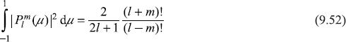
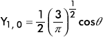
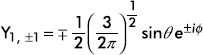
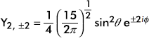
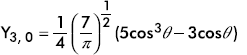
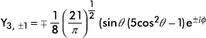
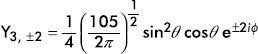
The expressions of a few normalized spherical harmonics Yl, m(θ, ϕ) are given in Table 9.1. Schematic plots of the distribution function |Yl, m(θ, ϕ)|2 are shown in Figure 9.2.
Figure 9.2 Schematic plots of the probability distribution |Yl, m(θ, ϕ)|2
We may summarize here the results about the eigenvalues of operators ![]() and
and ![]() . Whereas operator
. Whereas operator ![]() has eigenvalue l(l + l) ħ2, (l = 0, 1, 2, 3, ...), the z-component operator
has eigenvalue l(l + l) ħ2, (l = 0, 1, 2, 3, ...), the z-component operator ![]() has eigenvalues mħ (m = 0, ±1, ±2, 3, ... ±l). Therefore, for a fixed value of quantum number l (i.e. for a fixed magnitude of angular momentum vector |L| = l(l + 1) ħ2), the z-component of vector Lz may have (2l + 1) different values. In Figure 9.3, we show angular momentum vector L with a fixed value of Lz. In this case, L may point in any radial direction (with equal probability) along the surface of the cone of angle θ, where cosθ = Lz/L.
has eigenvalues mħ (m = 0, ±1, ±2, 3, ... ±l). Therefore, for a fixed value of quantum number l (i.e. for a fixed magnitude of angular momentum vector |L| = l(l + 1) ħ2), the z-component of vector Lz may have (2l + 1) different values. In Figure 9.3, we show angular momentum vector L with a fixed value of Lz. In this case, L may point in any radial direction (with equal probability) along the surface of the cone of angle θ, where cosθ = Lz/L.
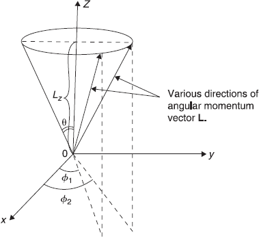
Figure 9.3 Angular momentum vector L with fixed value of Lz
If, for example, we consider a particular case of l = 2, then |L| = 1 (l + 1) ħ2 = 6 ħ2, and Lz may have various values 2ħ, ħ, 0, –ħ, –2ħ. This is shown in Figure 9.4.
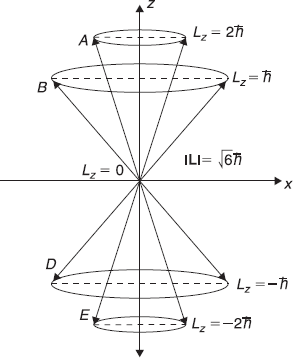
Figure 9.4 Angular momentum vector L corresponding to quantum number l = 2. Lz may have various values 2ħ, ħ, 0, –ħ and –2ħ (schematic diagram)
From the above findings it is clear that
- the three angular momentum component operators
 and
and  have simultaneous eigenstates with
  ;
; - the three component operators and do not have common eigenstates with one another except in a special case of zero angular momentum; and
- whenever L2 is measured along with one of the three components
 or
or  or
or  we find that
  (or or ).
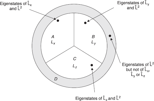
Figure 9.5 Venn diagram for the eigenstates of operators ![]() and
and ![]()
All these properties may be shown in a Venn diagram (Figure 9.5). In the Venn diagram, every point represents an eigenstate of operator ![]() . In sector A, every point is also an eigenstate of
. In sector A, every point is also an eigenstate of ![]() . Similarly, in sector B and C. Every point in the peripheral region D is an eigenstate of
. Similarly, in sector B and C. Every point in the peripheral region D is an eigenstate of ![]() only. The state at the centre is obviously the null eigenvector of
only. The state at the centre is obviously the null eigenvector of ![]() and
and ![]() . So, the state at the centre corresponds to the eigenvalues Lx = Ly = Lz = 0. In fact, we can note here that the (Venn) space of eigenstates of
. So, the state at the centre corresponds to the eigenvalues Lx = Ly = Lz = 0. In fact, we can note here that the (Venn) space of eigenstates of ![]() is bigger than the space containing all eigenstates of
is bigger than the space containing all eigenstates of ![]() and
and ![]() .
.
Table 9.1 First Few Normalized Spherical Harmonics
l |
m |
Spherical harmonics Yl, m(θ, ϕ) |
|---|---|---|
0 |
0 |
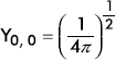 |
1 |
0 |
 |
±1 |
 |
|
2 |
0 |
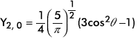 |
±1 |
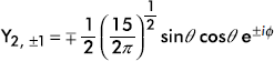 |
|
±2 |
 |
|
3 |
0 |
 |
±1 |
 |
|
±2 |
 |
|
±3 |
 |
9.6 MEASUREMENT OF ANGULAR MOMENTUM COMPONENTS AND THE UNCERTAINTY RELATIONS
The angular momentum component operators follow the commutation relations.
Using the result [Eq. (4.92)] of the generalized uncertainty relations in the present context, we have
Let us see what do the uncertainly relations like Eq. (9.54a) mean when we measure the angular momentum (components) in an experiment. Suppose, in an experiment we have measured L2 of the system (such as a particle, an atom, etc.). Then in the second measurement on the same system, it is possible to measure any one of the three Cartesian components of L, and leave the system with the same value of L2 that it had before the (second) measurement. That simply means that we can simultaneously know the precise values of L2 and of one of its components. Specifically, suppose we measure L2 and Lz and find the values 30ħ2 and 4ħ, respectively (getting the values of angular momentum quantum number l = 5 and azimuthal quantum number m = 4). Therefore, after both the measurements (i.e. the measurement of L2 and then that of Lz), the system is left in a (simultaneous) eigenstate of L2 and Lz, namely ψn, 5, 4.
Now, it is impossible to obtain more information about the vector L, without in any way destroying part of the information already obtained. For example, let one further measurement be done on the system to find value of Lx component. Suppose this measurement gives value 2ħ of Lx. But now value of Lz, which was obtained in the measurement (prior to the measurement of Lx) is no more 4ħ. In fact, now the value of Lz is totally uncertain. The system now is, in fact, in a (simultaneous) eigenstate of ![]() and
and ![]() . Since this is not an eigenstate of of
. Since this is not an eigenstate of of ![]() , a measurement now of Lz is not certain to yield any specific value. Similar is the case if instead of Lz, we choose to measure Ly. In fact, these observations are included in the uncertainty relation (9.54a), which in the present case gives
, a measurement now of Lz is not certain to yield any specific value. Similar is the case if instead of Lz, we choose to measure Ly. In fact, these observations are included in the uncertainty relation (9.54a), which in the present case gives
In the classical case, the angular momentum vector L may be completely determined. That means we can simultaneously know precise values of all the three components Lx, Ly, and Lz. In the quantum mechanical case, on the other hand, what can be known about L are the magnitude of L and value of only one of its components, say Lz. The other components, Lx and Ly, are not known simultaneously. We know that the relation ![]() holds even in quantum case. Therefore, knowing precise values of L2 and Lz also mean we know precise value of
holds even in quantum case. Therefore, knowing precise values of L2 and Lz also mean we know precise value of ![]() Now we shall have to make a picture of vector L such that (i) L2 and Lz have discrete values which are precisely known, (ii) Lx and Ly are not known precisely but
Now we shall have to make a picture of vector L such that (i) L2 and Lz have discrete values which are precisely known, (ii) Lx and Ly are not known precisely but ![]() has precise value. The picture which emerges is shown in Figure 9.3 (for the case of l = 2). For l = 2, L2 = 6ħ2 and Lz may have any one of the five values, 2ħ, ħ, 0, –ħ, –2ħ. The vector L points radially outwards, with equal probability, in any direction along the cone A for Lz = 2ħ case, along cone B for Lz = ħ, along cone D for Lz = –ħ, and along cone E for Lz = –2ħ. For the case of Lz = 0, the vector L points radially outwards in any direction in the x-y plane.
has precise value. The picture which emerges is shown in Figure 9.3 (for the case of l = 2). For l = 2, L2 = 6ħ2 and Lz may have any one of the five values, 2ħ, ħ, 0, –ħ, –2ħ. The vector L points radially outwards, with equal probability, in any direction along the cone A for Lz = 2ħ case, along cone B for Lz = ħ, along cone D for Lz = –ħ, and along cone E for Lz = –2ħ. For the case of Lz = 0, the vector L points radially outwards in any direction in the x-y plane.
9.7 ORBITAL ANGULAR MOMENTUM AND SPATIAL ROTATION
We would like to discuss here the relation between the angular momentum operator and the rotation operator. For this let us consider the passive rotation of the coordinate system about z-axis through an angle ∆ϕ (as shown in Figure 9.6). The transformation between the rotated coordinates (x′, y′, z′) and the original coordinates are given by
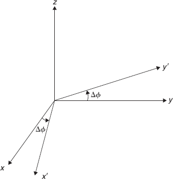
Figure 9.6 Passive rotation of Cartesian coordinate system about z-axis through an angle ∆ϕ
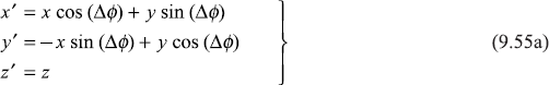
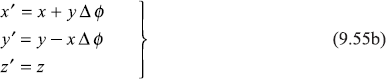
For infinitesimal rotation, ∆ϕ, the transformations are
We know that in the passive transformation (the rotation here), the coordinate system is transformed but the function [say, ψ(x, y, z)] is stationary. In active transformation, on the other hand, the coordinate system is fixed, whereas the function is transformed.
Let ![]() represent the rotation operator corresponding to the rotation of coordinate system about z-axis through an infinitesimal angle ∆ϕ. In this passive rotation of the coordinate system, the function ψ(x, y, z) is stationary in space, but in rotated coordinate system, this function is represented as ψ(x′, y′, z′), where x′, y′, z′ are given by Eq. (9.55). So
represent the rotation operator corresponding to the rotation of coordinate system about z-axis through an infinitesimal angle ∆ϕ. In this passive rotation of the coordinate system, the function ψ(x, y, z) is stationary in space, but in rotated coordinate system, this function is represented as ψ(x′, y′, z′), where x′, y′, z′ are given by Eq. (9.55). So
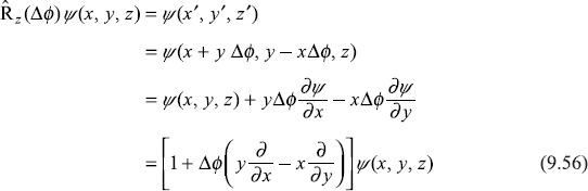
Here, we have retained only the first term of the Taylor expansion. Now, we know that the operator ![]() is given as:
is given as:
Therefore Eq. (9.56) may be written as
This equation states the relationship between the angular momentum component operator ![]() and the rotation operator
and the rotation operator ![]()
Similarly, we may have
Here, the operators ![]() may also be called as the generators of the infinitesimal rotations about the axes x, y, z, respectively. If we consider a general case of infinitesimal rotation of coordinate system through angle ∆ϕ about an axis along a unit vector e, the rotation operator Re(∆ϕ) is written as
may also be called as the generators of the infinitesimal rotations about the axes x, y, z, respectively. If we consider a general case of infinitesimal rotation of coordinate system through angle ∆ϕ about an axis along a unit vector e, the rotation operator Re(∆ϕ) is written as
We now proceed to find the expression for rotation operator ![]() corresponding to a finite rotation ϕ about the z-axis. Let us write ϕ = n∆ϕ and let n → ∞ and ∆ϕ → 0 such that ϕ is held constant. We can then write
corresponding to a finite rotation ϕ about the z-axis. Let us write ϕ = n∆ϕ and let n → ∞ and ∆ϕ → 0 such that ϕ is held constant. We can then write
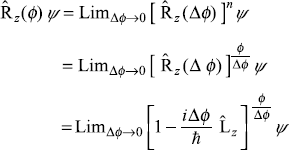
Putting ![]() we get
we get
Now using the definition of exponential ey = Limα→0 (1 + α)y/α, we have
It may be easily checked that the rotation operator Re(ϕ) for a finite rotation ϕ of the axes about unit vector e, is
Thus the wave function ψ(r′) in the rotated coordinate system, which was obtained by rotating the coordinate system about an axis along the unit vector e, through an angle ϕ may be written as
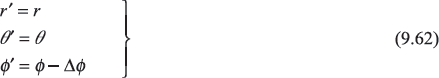
We can also work with rotation operator in the spherical polar coordinate system. For example, if we consider rotation about z-axis through an infinitesimal angle ∆ϕ, the transformation is given by
Therefore,
or
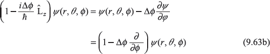
So, we get
or
EXERCISES
Exercise 9.1
Show that
Exercise 9.2
Show that
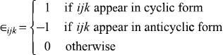
where symbol ∊ijk, called the Levi–Civita antisymmetric symbol, is defined as
Exercise 9.3
Show that
Exercise 9.4
Show that operators ![]() are Hermitian operators.
are Hermitian operators.
Exercise 9.5
Consider a particle of mass M constrained to move on a (frictionless) ring of radius a with its centre at 0 in x – y plane.
- Show that the Hamiltonian of the system is
 where I = moment of inertia of the particle with respect to the centre 0.
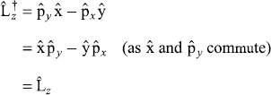
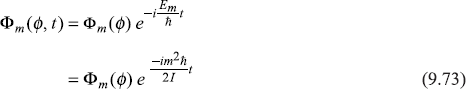
 - Find energy eigenfunctions of the system and write down the solution of time-dependent Schrodinger equation.
Exercise 9.6
Prove that
Exercise 9.7
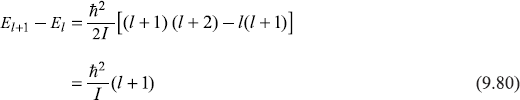
Imagine a diatomic molecule (at low temperature) as a rigid rotator; two particles (atoms) each of mass M separated by a weightless rigid rod of length 2a. The mid point of the rotator is fixed. Find the energy eigenvalues and eigenstates of the rotator.
In the above example, a diatomic molecule is considered as a rigid rotator. This corresponds to purely rotational modes of the molecule (when the vibration modes are absent, which happens at very low temperatures). Show that the frequencies of emitted photons due to transition between successive levels of rotational modes are given as
Exercise 9.9
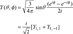
At a given instant of time, a rigid rotator is in the state
- What possible values of Lz will a measurement find and with what probabilities will these values occur?
- What is the value of
 for this state?
 - What is the value of
 for this state?
Exercise 9.10
We know ![]() Therefore,
Therefore,
Show that the following two assumptions imply directly the above result:
- Any component of L can have only values mħ (m = –l, –l + l, ...,+ l).
- All components of L are equally probable.
Exercise 9.11
If ![]() what is the value of
what is the value of ![]()
Exercise 9.12
Suppose that L2 is measured and the value of 12ħ2 is found. If Ly is then measured, what possible values can result?
SOLUTIONS
Solution 9.2
(a) We know the angular momentum component operator ![]() is expressed as
is expressed as
where i, j, k are in the cyclic order (i, j, k = 1,2, 3).
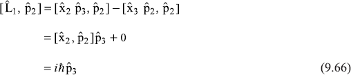
Let us firstly take commutator ![]() in cyclic order, say
in cyclic order, say ![]()
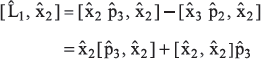
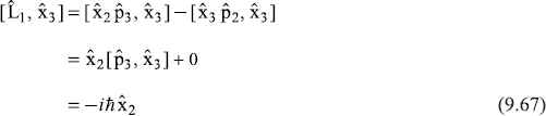
(b) Similarly, taking commutator ![]() in cyclic order
in cyclic order ![]() we have
we have
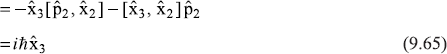
If next, we take the commutator ![]() in anticyclic order, say
in anticyclic order, say ![]() we have
we have
(b) Similarly, if we take the commutator ![]() in anticyclic order, say
in anticyclic order, say ![]() we get
we get
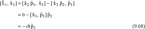
From Eqs (9.65) to (9.68) all the commutators of Example 9.1(a) may be obtained and the results are verified. Also the results of 9.1(b) may be verified. Here x1, x2, x3 mean x, y, z and P1, P2, P3 mean px, py, pz, respectively.
Solution 9.3
Similarly, other commutators may be evaluated.
We know
∴
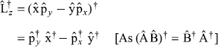
But we know that ![]() and
and ![]() are Hermitian operators
are Hermitian operators
∴
So, ![]() is Hermitian. Similarly,
is Hermitian. Similarly, ![]() and
and ![]() may be shown to be Hermitian.
may be shown to be Hermitian.
As ![]() where each component is Hermitian, so
where each component is Hermitian, so ![]() is also Hermitian. Next,
is also Hermitian. Next,
∴
so ![]() is Hermitian.
is Hermitian.
Solution 9.5
(a)
or
(b) We know that
The energy eigenvalue equation is
With Ĥ given by Eq. (9.69), above equation gives
Solution of time-dependent Schrodinger equation is given by the time-dependent wave function Φm (ϕ, t),
Solution 9.6
Putting the values of ![]() ,
, ![]() ,
, ![]() from Eqs. (9.18) in
from Eqs. (9.18) in ![]() we have
we have
Solution 9.7
As shown in Figure 9.7, the diatomic molecule is considered as a rigid rotator. The moment of inertia of the rotator about an axis, which is perpendicular bisector of the line joining two masses is
If we consider the rotator is far removed from any force field, its total energy is kinetic energy, which is
The corresponding Hamiltonian operator is
The time-independent Schrodinger equation of the system is
The eigenfunctions of Ĥ are the same as those of square angular momentum operator ![]() . Therefore, Eq. (9.77) may be rewritten as
. Therefore, Eq. (9.77) may be rewritten as
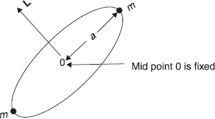
Figure 9.7 Diatomic molecule as a rigid rotator
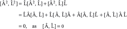
Solution 9.8
∴
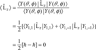
Solution 9.9
We may write
- Y(θ, ϕ) is an eigenstate of . The result of measurement of Lz in state Y(θ, ϕ) is same as the expectation value of in this state that is
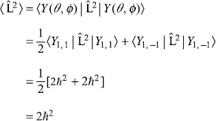
- We may easily check that

-
As all components are equally probable
Now all values of ![]() are equally probable, so
are equally probable, so
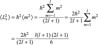
or
∴
Solution 9.11
Solution 9.12
so
So, if Ly is measured, the possible results are
REFERENCES
- Rose, M.E. 1957. Elementary Theory of Angular Momentum, New York: John Wiley.
- Gottfried, K. 1966. Quantum Mechanics. Vol. I, New York: W. A. Benjamin.
- Schiff, L.I. 1968. Quantum Mechanics, 3rd edn., New York: McGraw-Hill.
- Tinkham, M. 1964. Group Theory and Quantum Mechanics. New York: McGraw-Hill.
- Merzbacher, E. 1999. Quantum Mechanics. 3rd edn., New York: John Wiley.
- Bransden, B.H. and Joachain, C.J. 2000. Physics of Atoms and Molecules. 2nd edn., Upper Saddle River, NJ: Prentice Hall.