Chapter 14

WKB Approximation and Electron Tunnelling

14.1  INTRODUCTION

It may not be possible to solve Schrodinger equation exactly for a variety of potentials appearing in many practical cases. Therefore, one has to rely on methods which give approximate solutions of Schrodinger equation for such potentials. One class of approximate methods is the time-independent and time-dependent perturbation theory, which we shall discuss in the next two Chapters. In this Chapter, we confine ourselves to developing the approximate method of solving one-dimensional Schrodinger equation for the case where potential energy varies slowly with position. The method we shall discuss is called the WKB approximation, after G. Wentzel, H. A. Kramers, and L. Brillouin, who introduced it in quantum mechanics in 1926. It may be mentioned here that the method is generally applicable to one-dimensional problems. However, it may be applied to problems of higher dimensionality that are reducible to the solution of one-dimensional Schrodinger equation. The method is particularly useful in calculating bound state energies and in finding tunnelling rates through potential barriers. The WKB method is also called the classical approximation as it deals with situations, where ħ is small in comparison to the action involved.

14.2  THE ESSENTIAL IDEA OF WKB METHOD

Before describing the details of WKB approximation, in this section, we outline the main idea behind WKB approximation. Let us start with one-dimensional time-independent Schrodinger equation of a particle of mass m, moving in a potential V(x),

For energy E > V(x), the equation may be written as

where

For E < V(x), we get

where

Let us now imagine the particle moving through a region where potential is constant (say V₀). For E > V₀, the wave function of the particle is of the form

 

where

and A is a constant. The wave function ψ(x) is time-independent. However, if we write the corresponding time-dependent wave function

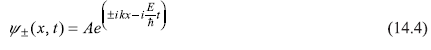
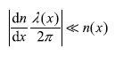
it becomes clear that the particle described by ψ₊ is travelling in +x direction and that described by ψ_– is travelling in –x direction. The wave function [Eq. (14.3a)] is representing a plane wave of fixed wavelength λ = 2π / k and fixed amplitude A. Now, let us consider a case where the potential V(x) is not constant but varying slowly with position such that the change in V(x) is very small over a distance of many wavelengths (see Figure 14.1). Therefore, in such a case, where V(x) is varying slowly, it is reasonable to assume that the wave function has the same form as in Eq. (14.3a), but k and A replaced by K(x) and A(x), the slowly varying functions of x. This is the main idea behind WKB approximation.

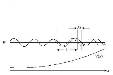
Figure 14.1 In WKB approximation . The potential scale of length should be large compared to λ. The dashed curve represents wave function for a constant potential and the solid curve is WKB wave function in potential V(x)

By same token, if E < V₀, the wave function ψ(x) is exponential

 

with

If in a region V(x) varies slowly with position such that change in V(x) is very small over a distance of then again the wave function remains of exponential form except that κ and A be replaced by κ(x) and A(x), the slowly varying functions of x.

14.3  DEVELOPMENT OF WKB APPROXIMATION

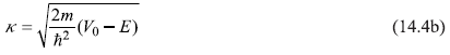
We start with one-dimensional Schrodinger equation [Eq. (14.1)]. The region where E > V(x) [and k(x) given by Eq. (14.2b) is real] is called the classical region, as a classical particle with its total energy E is confined to this region only (see Figure 14.2).

As discussed in Section 14.2, the WKB method manifests in starting with the solution of Eq. (14.2a) of the form

 

 

where we have to find out u(x) for the given potential V(x). We know that for the constant potential V(x) = V₀, u(x) = kx, that is, u(x) is simply linearly proportional to x. But for general V(x), u(x) may be complex function of x. Differentiating Eq. (14.5), we get

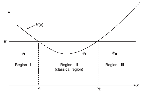
Figure 14.2 One-dimensional potential well. Classically, the particle is confined to region-II, where E > V(x). x₁ and x₂ are the turning points

Substituting Eqs (14.5) and (14.6b) in Eq. (14.2a), we get

Till now we have made no approximations and the solution given by Eq. (14.5) is exact, provided u(x) is the exact solution of Eq. (14.7). However, Eq. (14.7) is not solvable exactly in most of the cases and some approximations will be made to solve it.

We know that for the constant potential V(x) = V₀, (d²u/dx²) = 0 and, therefore, if V(x) varies slowly with x, (d²u/dx²) must be a small quantity. As a first approximation, we neglect (d²u/dx²) in Eq. (14.7) and get first (crude) approximation u₀ to u

On integration, it gives

Having found u₀(x) one may find [d²u₀(x) / dx²] and put it in Eq. (14.7) [in place of (d²u/dx²), which was taken to be zero in the above treatment] to get

Equation (14.10) gives improved value of u in comparison to that given by Eq. (14.8). Let us call it u₁, so

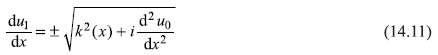
Integrating it, we get

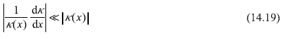
In writing solution [Eq. (14.12)], it is presumed that the term (written for [d²u_o(x)/dx²] is quite small in comparison to k²(x), that is,

or

or

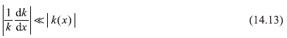
We shall analyse this condition in details a bit later. Under the said condition, the integrand in Eq. (14.12) may be expanded binomially to give

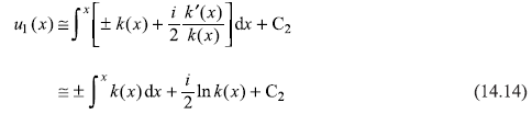
So u₁(x) given by Eq. (14.14) is an approximate solution of Eq. (14.7). When put in Eq. (14.5), we get WKB wave function

 

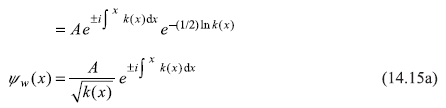
It can be noted from Eq. (14.15a) that

where linear momentum So Eq. (14.15a) dictates that the probability density of finding the particle at x is inversely proportional to its classical linear momentum and hence to its velocity at x. This is what really one expects in the motion of a classical particle. The particle spends less time in a region where its velocity is large. And, therefore, the particle is less probable to be found in that region. That is why sometimes WKB approximation is known as semi-classical approach.

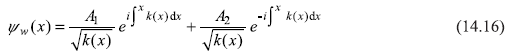
Turning now to the solution Eq. (14.15a), the general WKB solution should be a linear combination of two such terms, one with positive and the other with negative sign, that is,

In arriving at the WKB solution, we have considered E > V(x) i.e. k²(x) as positive. However, for E < V(x), the quantity κ²(x), defined through Eq. (14.2d), that is

 

 

is positive and the corresponding Schrodinger equation is given by Eq. (14.2c). Using a similar method as used above to arrive at Eq. (14.16) for E > V(x), we may obtain following WKB solution for E < V(x) case:

For E < V(x), a condition similar to that of (14.13) may be obtained for validity of WKB approximation, given by

14.4  VALIDITY OF WKB APPROXIMATION

Let us start with the WKB solution given in Eq. (14.15a). Differentiating Eq. (14.15a) twice, we get

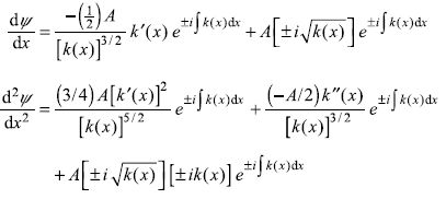
or

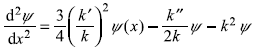
or

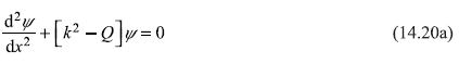
where

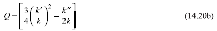
Equation (14.20a) is an approximation to the Schrodinger equation [Eq. (14.2a)] if Q is very small. That means the WKB wave function is the solution of Schrodinger equation [Eq. (14.2a)] if

or

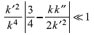
or

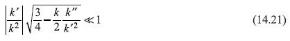
Condition (14.21) is equivalent to condition (14.13).

Let us analyse the condition (14.13) in a bit more detail:

1. For a slowly varying potential V(x) (Figure 14.1), solid curve shows the WKB wave function. The dashed curve shows the wave function for a constant potential. For a slowly varying potential, the change in wave length over the distance of one wavelength shall be very small in comparison to the wavelength itself, that is
   

   or

   

   Now k = (2π / λ) and, therefore, condition (14.22) becomes same as (14.13).

2. We have from Eq. (14.2b)
   

   so condition (14.13) becomes

   

   or

   

   which means condition (14.13) is fulfilled for problems where

   1. mass of the particle is large,
   2. energy E is high, and
   3. the potential V(x) is smoothly varying.
3. Let us see what does the condition (14.13) mean (in electromagnetic theory) when a plane monochromatic electromagnetic wave propagating in x-direction is incident on an inhomogeneous medium with varying refractive index n(x). We know the relation in the medium
   

   whereas in vacuum

   

   Here ω is the angular frequency of electromagnetic wave and c is velocity of light in vacuum. Equation (14.13) for the present case gives

   

   If we omit the factor of 2π, it gives

   

So WKB method is well applicable to the case of electromagnetic wave propagating in an inhomogeneous medium if the change in refractive index in a distance of one wavelength is very small.

14.5  THE CONNECTION FORMULAE

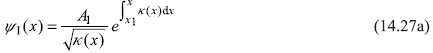
Let us consider the potential V(x) of the form shown in Figure 14.2; classically, the particle of energy E is confined to region-II. In quantum mechanical description the particle is found in region-I and region-III as well. In region-I, the wave function of the particle decreases exponentially as x → –∞. In this region ψ(x) is approximated by

In region-II, the wave function is oscillatory and can be written as

In region-III, the wave function decreases exponentially as x → ∞ and can be written as

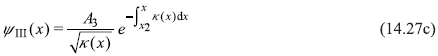
In Figure 14.2, x₁ and x₂ are the classical turning points spanning the so-called classical region. The WKB approximation breaks down in the vicinity of these points as |k²(x)| is very small around classical turning points (see Figure 14.3). Therefore, the WKB wave functions, Eqs (14.27a,b,c), are asymptotically valid because these are valid only in regions away from the turning points x₁ and x₂. In the regions around the turning points, the wave functions will be found by solving Schrodinger equation without WKB approximation. In fact, for slowly varying potentials V(x), it may be approximated as linearly varying in the neighborhood of x₁ and x₂. So we write near x₁,

 

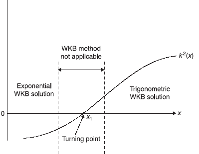
Figure 14.3 Variation of k²(x) where exponential solutions are to the left of the classical turning point at x = x₁ and trigonometric solutions to the right of x₁. WKB method is not applicable in the vicinity of x₁

and near x₂

 

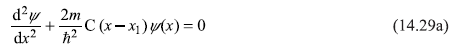
The Schrodinger equation [Eq. (14.2a)] near x₁ becomes

and near x₂

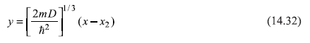
With the change of variable

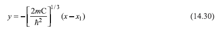
Equation (14.29a) gives

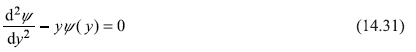
In a similar way, the change of variable

changes Eq. (14.29b) in the form of Eq. (14.31). Now suppose the Schrodinger equation [Eq. (14.31)] has been solved and we have got expressions of wave function for x in the neighborhood of x₁ and x₂. So we have got WKB wave functions in region I, II, III (except in the neighbourhood of x₁ and x₂) and also wave functions in the neighborhood of x₁ and x₂ by solving Schrodinger equation [Eq. (14.31)]. Since the final wave function has to be continuous and smooth for all x, it should be possible to obtain connection formulae which allow us to join WKB solutions in three regions across the turning points. We shall not do this exercise here. We shall borrow the connection formulae from, for example, Merzbacher (Quantum Mechanics, 1999) and Powell and Crasemann (Quantum Mechanics, 1961) who have solved Schrodinger equation [Eq. (14.31)] in terms of Airy functions and developed connection formulae.

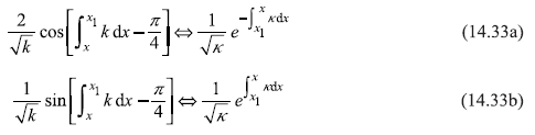
The connection formulae, at the turning points x₁ and x₂ are given below:

Connection formulae at x = x₁ (Figure 14.4)

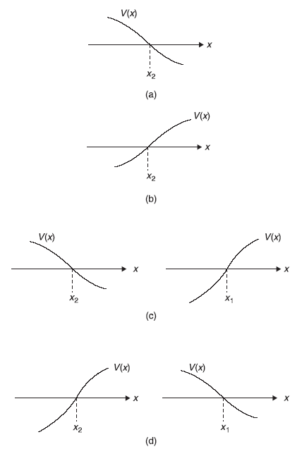
Figure 14.4 (a, b) Showing turning points x₁ and x₂ (c) Point x₂ happens to be in left of x₁ for the potential well (d) x₂ is on right side of x₁ for potential barrier

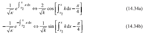
Connection formulae at x = x₂ (Figure 14.4)

14.6  APPLICATION OF WKB TECHNIQUE TO BARRIER PENETRATION

We had solved the problem of penetration of a rectangular barrier in Section 5.7. However, if the barrier has a complicated shape, the corresponding Schrodinger equation may not be solved exactly and we have to resort to the approximate methods. We shall see that WKB method may be very well applied to such problems.

Let us consider a potential barrier V(x) as shown in Figure 14.5. Let a beam of particles be incident from left with energy E (E < V₀, the top of the barrier). As shown in the figure, there are two turning points x₁ and x₂. The three regions I, II, and III correspond respectively to x < x₁, x₁ < x < x₂ and x > x₂. Some of the incident particles are reflected back and some are transmitted through the barrier to region-IIΙ. Now the transmitted wave in region-III has only one momentum component and the wave function within WKB approximation may be written as

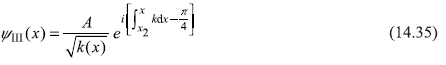
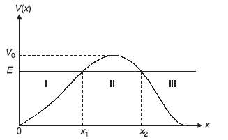
Figure 14.5 Transmission through a potential barrier

The transmission coefficient is obtained once we know the incident component of the wave function in region-I and the transmitted wave function in region III. The transmitted wave function ψ_III(x) is given in Eq. (14.35). We shall find the incident component ψ_I(x) in following manner:

1. Firstly, we shall rewrite ψ_III in terms of trigonometric (sine and cosine) functions to enable us to use connection formulae [Eqs (14.34)] at turning point x₂ to write ψ_II(x).
2. After knowing ψ_II(x), we rewrite it in such a form that connection formulae [Eq. (14.33)] may be used at the turning point x₁ to connect ψ_II(x) to ψ_I(x).
3. Finally, the incident component is extracted from ψ_I(x) by decomposing it into incident and reflected parts.

So let us decompose wave function ψ_III(x) as

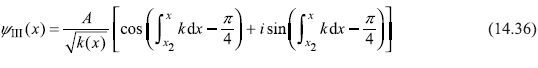
Using connection formulae [Eqs (14.34)] at turning point x₂, the terms in Eq. (14.36) may be connected to write ψ_II(x) as follows

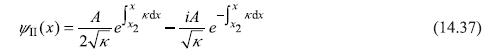
where

If we look at the two terms of Eq. (14.38), the first term increases exponentially as x increases whereas the second term decreases on increasing x. Now as the beam of particles is incident from left, the amplitude of the wave function is bound to decrease exponentially as x increases (from x₁ towards x₂), so the second term in Eq. (14.38) is the only significant term for ψ_II(x). Therefore,

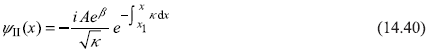
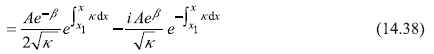
In order to find the appropriate wave function ψ_I(x) in region-I, we apply connection formulae [Eqs (14.33)] at point x₁ to arrive at

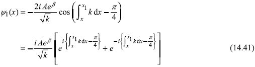
Here the first term in the square bracket is representing a wave moving to the right while the second one represents that moving to the left. So the first term corresponds to the incident wave.

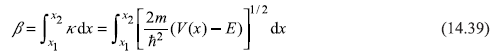
Now it is easy to find the transmission coefficient T. as discussed in Chapter 5. The transmission coefficient is the ratio of the transmitted probability current density to that of the incident probability current density. From the WKB wave functions ψ_III(x) [Eq. (14.35)] and ψ_I(x) [incident wave part of Eq. (14.41)], we may find the expression of T under WKB approximation as

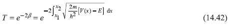
It may be mentioned here that WKB method of finding wave functions and therefrom transmission coefficient gives reasonable results only when

1. the potential V(x) is slowly varying, and
2. the turning points x₁ and x₂ are sufficiently well separated such that the barrier thickness (x₂ – x₁) is of several wavelengths.

Under these conditions, the quantity β given in Eq. (14.39) must be large, resulting in a small value of T [Eq. (14.42)]. So the reflection coefficient R = 1 – T shall be very close to unity. In fact, the two terms in ψ_I(x) in Eq. (14.41) (representing the incident and the reflected components) have same amplitude and, therefore, given reflection coefficient R to be exactly unity.

It is interesting to compare the WKB result of transmission through a rectangular potential barrier with the results obtained by the exact solutions of Schrodinger equation (Section 7.5). The WKB result of transmission coefficient for incident particles of energy E for the rectangular barrier of height V₀ and thickness L is [from Eq. (14.42)].

 

where

In the limit , the transmission coefficient for the said rectangular barrier, obtained in Section 5.7, is given as

The WKB result is in good order of magnitude agreement with the limiting value of the exact result.

14.7  COLD EMISSION OF ELECTRONS FROM METALS

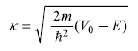
We have studied the transmission probability of a particle through a potential barrier using WKB approximation. We shall now study in this section the tunnelling of conduction electrons out of metal in presence of an external pulling force on electrons due to applied external electric field using WKB method. We discussed the free electron model of conduction electrons in simple metals in Sections 10.3 and 10.4. It was discussed there that the conduction electrons in metals are just like electrons in a three-dimensional potential well of finite depth. The free electron energy levels are very closely spaced and can be described through the density of states D(E). At temperature T = 0 K, all levels up to Fermi energy E_F are filled (each state is, in fact, occupied by two electrons; one with spin up and the other with spin down). All levels above Fermi energy are unoccupied. The difference between the top of well V₀ and the Fermi energy E_F is really the minimum energy (W) required to remove an electron from metal. W is called the work function of the metal (see Figure 14.6).

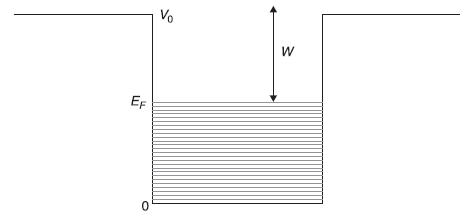
Figure 14.6 Free electrons in a metal. At temperature T = 0 K, all levels up to Fermi energy E_F are filled. An electron with Fermi energy requires energy W (called the work function of metal) to take it out of metal

Figure 14.7 A metal cube in presence of a constant homogeneous (external) electric field E = – E₀ e_x in -x direction. The force on electrons is F = | e | E₀e_x in +x direction

 

Let us now assume that a constant homogeneous electric field E = –E₀e_x is applied to the metal (as shown in Figure 14.7). This field pointing in –x direction exerts a constant force F = eE₀e_x on electrons in +x direction. This is equivalent to the additional potential energy of electrons V(x) = – E₀ x (x is the distance from the surface of the metal). Therefore, while in the absence of external electric field, the electrons have potential V₀ for x > 0 (as shown in Figure 14.8a), in the presence of field, the electrons have potential V(x) = V₀ – eE₀x (shown in Figure 14.8b). Thus, the potential barrier now has a finite width (as seen in Figure 14.8b), so that electrons may tunnel through and escape from the metal. The phenomenon is called as field emission or cold emission of electrons. However, if the metal is at high temperature, a fraction of the electrons are in higher energy states. Some electrons may acquire enough energy to overcome the barrier, even in absence of external electric field. This phenomenon is called as thermal emission.

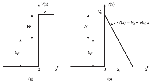
Figure 14.8 (a) Thick solid line represents the potential binding the electrons in a metal (b) Potential energy in presence of an external electric field E₀. x₁ is the classical turning point for an electron with energy E_F

We now proceed to find an estimate of the transmission coefficient T of electrons at Fermi energy E_F. For electrons with energy E_F = V₀ – W, the turning point x₁ is given as

 

or

The other turning point is at the surface of the metal itself, that is x₂ = 0. Thus using the WKB expression [Eq. (14.42)] for transmission coefficient alongwith x₁ = W/eE₀, x₂ = 0, V(x) – E = V(x) – E_F = V₀ – eE₀x – E_F = W – e E₀ x, we have

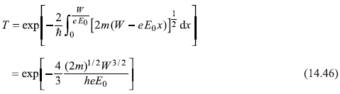
This is known as Fowler–Nordheim cold emission (or field emission) formula and agrees with the experimental data.

14.8  ALPHA-DECAY OF NUCLEI

In this section, we would like to use the results of WKB approximation for the transmission coefficient, to calculate the lifetime of nuclei emitting alpha particles. The potential energy of an alpha particle is shown schematically in Figure 14.9. When inside the nucleus (r < R), the α-particle is acted upon by strongly attractive nuclear forces. The precise form of this nuclear force may not be known and, moreover, the precise form is not needed at the level of WKB approximation. Therefore, for simplicity, we represent it by a square well potential of depth V₀ (for r < R). Outside the nucleus (r > R), the short range nuclear forces are negligible and the only force α-particle, with change 2e, experiences is the Coulomb repulsion with the daughter nucleus with change Ze. Therefore, the potential energy V(r) of the α-particle is approximated by

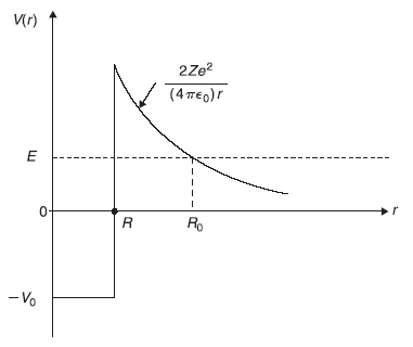
Figure 14.9 Schematic plot of potential energy of an α-particle inside and outside a nucleus of radius R. r = R₀ is the classical turning point of α-particle of energy E

 

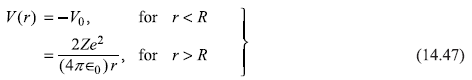
In writing Eq. (14.47), we have assumed that a parent nucleus of charge (Z + 2)e decays to a daughter nucleus of charge Ze by emitting an alpha-particle of charge 2e. The potential energy shown in Figure 14.9 corresponds to the case where α-particle is free inside the nucleus and is bound by sharply attractive nuclear forces. As Coulomb potential effectively vanishes in the region where r is large, in this region kinetic energy of α-particle is equal to its total energy E. So an α-particle with total energy E may not be considered in a bound state inside the nucleus. The α-particle of energy E shall penetrate the potential barrier in the region from r = R to r = R₀, such that E = V(R₀). From Eq. (14.47), we have

To make the problem simple and reducible to one-dimensional problem, let us assume that the α-particle is in state of zero angular momentum. Now using spherical polar coordinates, we may write its wave function in form [u(r)/r]. Then the function u(r) [= u_l=0(r)] satisfies the radial equation

where M is the mass of α-particle (note that α-decay takes place in heavy nuclei, so the reduced mass is almost equal to M). Now Eq. (14.49) is identical to the one-dimensional Schrodinger equation [Eq. (14.1)]. So we may get the expression of transmission coefficient T for penetration of potential barrier by using one-dimensional WKB result [Eq. (14.42)]

 

where

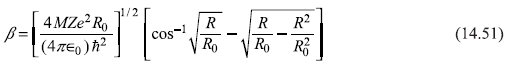
Using Eq. (14.48), we may write β in the form

With the substitution r = R₀ cos² θ, we can easily integrate (14.50c) to get

As nuclear forces are short ranged, the quantity (R/R₀) << 1, so we may write

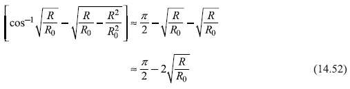
as for small x, cos^–1 x ≈ (π/2) – x. Therefore, we get

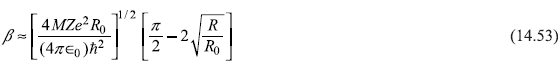
or

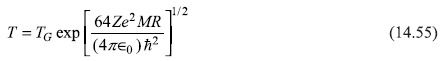
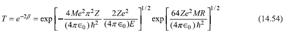
where

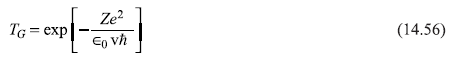
Here we have used Eq. (14.48) to express R₀ in terms of energy E. Then energy E is expressed as Mv²/2, where v is the velocity of α-particle with which it emerges. The quantity T_G is known as Gamow factor.

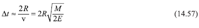
The lifetime of the nucleus emitting α-particle may be estimated from the expression of transmission coefficient [Eq. (14.54)]. To have a rough estimate of the lifetime, we take a simple picture of α-particle inside the nucleus. We imagine the α-particle confined in a potential well and being bounced back and forth by the potential walls before its emission from the well/nucleus. Now the transmission coefficient T is really the probability of (α-particle) getting through the barrier on a single collision with the wall. Therefore, the number of collisions required to get α-particle out of the barrier is of the order of T^–1 (as total probability of tunnelling, P = probability of tunnelling in one collision × number of collisions = T × T^–1 = 1). Now the time interval between successive collisions (∆t) should be roughly equal to the diameter of the nucleus (2R) divided by the speed , that is

If τ is the lifetime of the nucleus, that is, α-particle stays inside nucleus for time τ, it will make (τ/∆t) collisions during this time, which should be equal to T^–1 to make its successful exit from the nucleus, that is

or

Using Eq. (14.54) for T, we may express τ as

where we can easily identify and evaluate positive constants, A, B, and C. Now the first term depends on energy E in a logarithmic way and hence is a weak-dependence in comparison to the second term. We may treat first term to be almost constant and can combine it with the third term. So we may write

In other words, the energy dependence of lifetime τ is almost entirely governed by the term B E^–1/2, which means τ depends entirely on the tunnelling through the barrier. From the experimental data on a large number of alpha-radioactive nuclei, it has been seen that the relation between lifetime τ of radioactive nuclei and the kinetic energy E of the emitted α-particle are related with each other in the same way as given by Eq. (14.60).

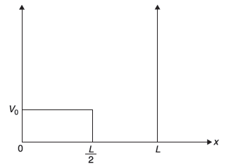
Figure 14.10 Half the well perturbed by constant potential V₀

EXERCISES

Exercise 14.1

Consider a particle in an infinite one-dimensional well, with the potential

 

shown in Figure 14.10 above. Find out allowed energy eigenvalues and eigenstates for energy E > V₀, within WKB approximation.

Exercise 14.2

An electric field E is applied normal to the sodium metal surface. Estimate the field strength E necessary to draw current density of the order of one mA/cm² from the sodium metal surface. For J_inc, you may use the expression J_inc = nev, where v may be taken as Fermi velocity v_F. (Given data for sodium metal: n = 2.65 × 10²⁸ / m³, v_F = 1.07 × 10⁶ m/s, work function W = 2.35 eV).

SOLUTIONS

Solution 14.1

We have from Eq. (14.16)

or more conveniently

where

and

Now ψ_w(x) must go to zero at x = 0, therefore,

 

 

Also ψ_w(x) must go to zero at x = L, therefore,

 

 

or

 

 

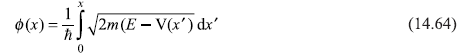
so from (14.64), we get

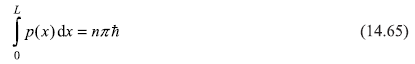
This quantization condition determines the (approximate) allowed energy eigenvalues and corresponding eigenstates [from Eq. (14.62b)].

For the given potential (14.61), Eq. (14.65) gives

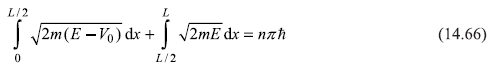
or

squaring it, we get

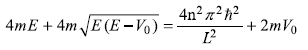
or

or

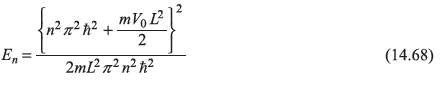
For V₀ = 0, we get

which matches with the exact result of eigenvalues of a particle in a potential box of width L.

Solution 14.2

The field emission current density J_field is obtained as

 

 

where T is the transmission coefficient given by Eq. (14.46) as

From the given data

 

 

We want to get J_field ≈ 1.0 m A/cm². So T should be

From Eqs (14.71) and (14.72)

 

REFERENCES

1. Gasiorowicz, S. 1996. Quantum Physics, 2nd edn. New York: JohnWiley.
2. Powell, J.L. and Crasemann, B. 1961. Quantum Mechanics. MA: Addison-Wesley.
3. Fromhold Jr., A.T. 1981. Quantum Mechanics for Applied Physics and Engineering. New York: Academic Press.
4. Merzbacher, E. 1999. Quantum Mechanics, 3rd edn. New York: John Wiley.