Appendix A

Early Quantum Mechanics

There were a few experimental observations, towards the end of nineteenth century that could not be explained on the basis of the then well-established classical concept/mechanics. One was the discrete energy spectrum of hydrogen atom and the other was the intensity distribution of black body radiations. In 1900, Planck came forward with an innovative idea of discrete energy levels of harmonic oscillator, and was able to explain black body energy distribution. In 1913, Bohr put forward his atom model of discrete values of angular momentum of electrons, and was able to explain many features of discrete energy spectrum of hydrogen atom. Here we review, in brief, these early developments.

A.1  PLANCK’S FORMULA OF BLACK BODY RADIATIONS

We know that at finite temperature T, the ions in the walls of the black body cavity oscillate and as a result emit electromagnetic radiations. The ions continuously emit and absorb electromagnetic radiations. Planck came up with a revolutionary quantum hypothesis that the oscillators emit and absorb energy in discrete unit of energy ∊, so that the only available energy states of these oscillators are those for which E = 0, ∊, 2 ∊, ...

Now, the probability of an oscillator at temperature T to have energy E is given by the Boltzmann factor e^−E/KT, where k is the Boltzmann constant. Therefore, on the basis of Planck’s hypothesis, the average energy of the oscillator is given by

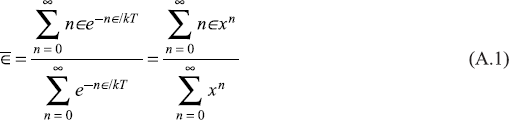
where

 

 

Using the formulae

and

the average energy is

The energy ∊ of the oscillator, called as quanta of energy was supposed to have value

 

 

where v is the frequency of the oscillator and h is Planck’s constant. Now, the oscillators (or strictly speaking lattice vibrations) of the walls of the cavity container have a large number of frequencies. So the quanta of energy hv corresponding to the frequency v of the oscillator is emitted (to the e.m. radiation field of the cavity) and absorbed (from the e.m. radiation field present in the cavity).

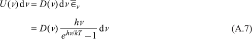
We have found out the average energy of an oscillator of frequency v to be 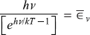(say),which is, in fact, same as the average energy of a radiation oscillator of frequency v (or the e.m. field of frequency v in the cavity). Therefore, to find intensity spectrum of the e.m. field in the cavity, we should find out number of modes of e.m. waves in between the frequency interval v and v + dv. Let us call this number as D(v)dv. So the energy of the radiation field within the frequency range v and v + dv is

To find D(v): Let us assume the cavity of cubic shape with side L. Let us assume the periodic boundary conditions on the electromagnetic waves in the cavity in x, y, and z directions. That simply means an integral number of wavelengths must fit into the length L. So, an e.m. plane wave e^ik.r, obeying periodic boundary conditions, must obey the relations

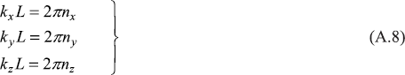
or

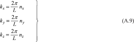
Here

 

 

is the wave vector of the e.m. wave. Condition (A.9) may be written as

when n is a set of three integers {n_x, n_y, n_z}. Therefore, the total number of allowed modes for which wave vector is in the range k and k + dk, is

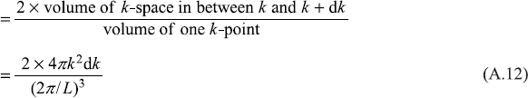
Here, factor of 2 is there because of two directions of polarizations (of e.m. wave). For e.m. radiations, we have the relation

Therefore,

Putting this in Eq. (A.12), we get for the number of allowed modes

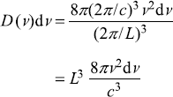
And number of modes per unit volume of cavity

Putting Eq. (A.14) in Eq. (A.7), we get

This law is in complete agreement with the experimental results.

A.2  ATOMIC SPECTRA AND BOHR’S MODEL OF HYDROGEN ATOM

By the end of nineteenth century, the hydrogen atom emission spectrum was found having spectral line series such as Balmer series in the visible and near ultraviolet region. In 1913, Bohr was able to explain the presence of these lines on the basis of a model, now known as Bohr Atom Model. Bohr combined the concepts of Rutherford’s nuclear atom, Planck’s quanta, and Einstein’s photon to explain the observed spectrum of hydrogen atom.

Bohr assumed that an electron in an atom moves in a circular orbit centered at the nucleus under the influence of the electrostatic attractive force of the nucleus. Bohr postulated that only a certain set of stationary states are allowed, which have discrete energy values. As long as an electron is in a stationary state/orbit, it does not radiate e.m. energy. Radiation is emitted only when an electron makes a transition from one allowed energy level to another. Bohr obtained the frequency of the radiation by making use of the idea that the energy of e.m. radiation is quantized. The quantum of energy is called as photon, and each photon associated with frequency v has energy hv. Therefore, if the electron makes a transition from a level of energy E_a to a level of energy E_b, the emitted photon shall have frequency v given by

 

 

This is known as Bohr’s frequency relation.

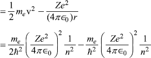
Let us apply these ideas of Bohr to get values of frequencies of the radiations emitted by an atom. Let the mass and charge of electron be denoted by m_e and (–e), respectively, and the nuclear charge by +Ze. Let the nucleus be assumed to be at rest at the origin (of the coordinate system). If the electron is moving with non-relativistic velocity v in a circular orbit of radius r, the centrifugal force (m_ev²/r) must be balanced by electrostatic attractive force by the nucleus, so

Bohr postulated that the orbital angular momentum of the electron is quantized

 

 

From Eq. (A.17) and Eq. (A.18), we obtain the allowed values of v and r as

It may be seen that if we put Z = 1, n = 1, the radius of first orbit of hydrogen atom has value

a₀ is generally known as Bohr radius.

The total energy of the electron in bound state with quantum number n is given as

 

or

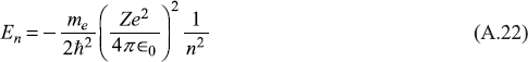
Let us use Bohr’s frequency relation (A.16) to find the frequencies of the spectral lines corresponding to transitions from energy level E_a to level E_b:

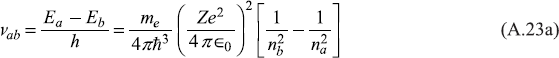
Here n_a > n_b. The corresponding wave numbers are For hydrogen atom Z = 1, so we get

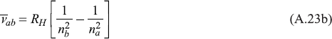
where

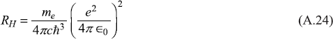
is called Rydberg constant. If we put values of constants in Eq. (A.22), we get

 

 

This simple model of Bohr is able to explain qualitatively main features of hydrogen atom spectrum.

A.3  BOHR’S CORRESPONDENCE PRINCIPLE

Bohr developed quantum theory of atom in 1913, which was able to explain main features of hydrogen atom spectrum. In 1923, Bohr put forward an idea which suggested that the quantum theory should merge into classical theory in the limit in which classical theory was known to apply. This idea was formulated as correspondence principle. Technically it states that the classical limit should be reached when the ‘quantum numbers’ involved are large. In fact, this principle has been helpful in guiding theoretical guesses in quantum mechanics such that for large quantum numbers, we should get quantum results merging with classical results.

As an example, let us see how the correspondence principle is satisfied by Bohr atom model, when the frequency of emitted radiation is considered for transition from orbit with quantum number n to orbit with quantum number n – 1, n being very large. When n is large, the angular momentum nħ is indeed very large in comparison to ħ and, therefore, may be in classical domain. According to classical electrodynamics, an electron moving in a circular orbit with velocity v would radiate with the frequency of its rotational motion, i.e.

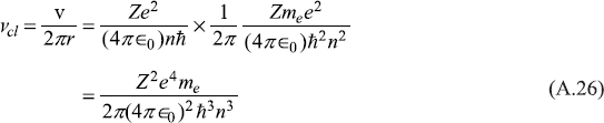
On the other hand, the frequency of radiation emitted when the electron makes a transition from energy level E_n to that immediately below, E_{n – 1}, is given by

When n is large, we have [1/(n – 1)² – (1/n²) ≈ (2/n³)], so

which is same as classical result [Eq. (A.26)].

A.4  THE FRANCK-HERTZ EXPERIMENT

It was shown in Planck’s work on black body radiation (1900) and Einstein’s study of photoelectric effect (1905) that the electromagnetic radiations when interacting with matter behave like an assembly of discrete quanta of energy and not like an extended continuous wave. On the other hand, Bohr’s model of hydrogen atom (1913) put forward the idea of discrete energy levels of electrons in an atom. In 1914, Franck and Hertz did an unusually elegant experiment which proved that mechanical energy, like electromagnetic energy, is absorbed by atoms in discrete quanta. This experiment provided an excellent confirmation of the discrete nature of energy levels of atoms.

The schematic diagram of the apparatus used by Franck and hertz is shown in Figure A.1. The electrons are ejected from electrically heated cathode C in an evacuated tube and are accelerated towards grid G maintained at a positive potential V₁ with respect to the cathode C. The electrons attain a kinetic energy Some of these pass through the grid and reach the plate P, thus forming a current I in plate circuit. The plate is, in fact, at a slightly lower potential V₂ than the grid. Therefore, electrons moving in between grid G and plate P experience a retarding potential ∆V = V₁ – V₂ (∆V << V₁). The retarding potential ∆V reduces the kinetic energy of electrons slightly.

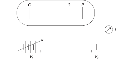
Figure A.1 Apparatus for the Franck-Hertz experiment

After evacuation, the tube is filled with mercury vapour. If there were no vapour, the current I will go on increasing with increasing V₁. In presence of vapour, the electrons will collide with mercury atoms, and if the collisions are elastic, the current will be unaffected by the introduction of the gas. This is because mercury atoms are too heavy to gain any appreciable kinetic energy. However, if an electron makes inelastic collision with mercury atom, thereby loosing energy E in exciting mercury atom, its kinetic energy will reduce to If this kinetic energy is very small, the retarding potential will be sufficient to prevent the electron from reaching the collecting plate P. Thus the current I will decrease.

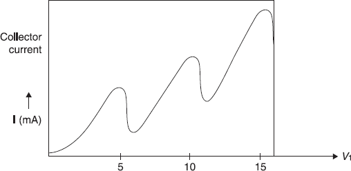
Figure A.2 Variation of collector current with voltage

When the experiment was carried out and current I was measured as a function of V₁, the current (shown schematically in Figure A.2) suffered a sharp decrease at a potential V₀, which for mercury was found to be 4.9 V. As discussed above, this result may be understood by assuming that mercury atom has its first excited energy level 4.9 eV above its ground state level. So, electrons having energy, eV₁ lesser than 4.9 eV are not able to excite mercury atoms, and their collision with mercury atoms is elastic. When eV₁ reaches the value 4.9 eV, a number of electrons (with energy 4.9 eV) collide with mercury atoms inelastically, transfer their energy to excite mercury atoms. As a result, such electrons are left with negligible energy not able to reach the plate. Thus current I decreases drastically. When voltage V₁ is increased further, current I increases, but again suffers sharp dips. These dips in current may be due to the excitation of mercury atoms to higher energy levels or due to multiple collisions of an electron with atoms, each time exciting atoms to their first (excited) level.

Therefore, the Frank–Hertz experiment provides an excellent confirmation of the discrete energy level in atoms.