CHAPTER  3

Hidden Performance Gotchas

By Gail Shaw

Performance tuning is often considered to be one of those dark arts of Microsoft SQL Server, full of secrets and mysteries that few comprehend. Most of performance tuning, however, is about knowing how SQL Server works and working with it, not against it.

To that end, I want to look at some not-so-obvious causes of performance degradation: predicates, residuals, and spills. In this chapter, I’ll show you how to identify them and how to resolve them.

Predicates

The formal definition of a predicate (in the database sense) is “a term designating a property or relation,” or in English, a comparison that returns true or false (or, in the database world, unknown).

While that’s the formal term, and it is valid, it’s not quite what I want to discuss. Rather, I want to discuss a situation where during the query execution process, SQL evaluates the predicates (the where clause mostly) and how that can influence a query’s performance.

Let’s start by looking at a specific query:

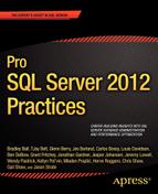
That’s very simple: two tables, two predicates in the where clause, and one in the from (the join predicate). Figures 3-1 and 3-2 show two execution plans from that query’s execution.

Figure 3-1. Execution plan 1.

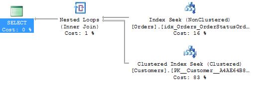
Figure 3-2. Execution plan 2.

At first glance, those two execution plans look pretty much the same, except for some slight differences in the relative cost percentages. They also look rather optimal (with two index seeks and a loop join). But what if I tell you that the execution statistics for the two executions were quite different?

Execution plan 1:

Table 'Worktable'. Scan count 0, logical reads 0.

Table 'Orders'. Scan count 1, logical reads 5.

Table 'Customers'. Scan count 1, logical reads 4.

SQL Server Execution Times:

  CPU time = 0 ms, elapsed time = 1 ms.

Execution plan 2:

Table 'Worktable'. Scan count 0, logical reads 0.

Table 'Orders'. Scan count 1, logical reads 301.

Table 'Customers'. Scan count 1, logical reads 4.

SQL Server Execution Times:

  CPU time = 0 ms, elapsed time = 4 ms.

You can see that there are 5 reads against the Orders table in execution plan 1, compared with 301 reads against the Orders table in execution plan 2, and both are index seek operations. What causes that difference?

Quite simply, it has to do with when, in the execution of the index seek, SQL Server evaluates the predicates. Let’s take a closer look at the execution plans—specifically, at the properties of the index seek (as shown in Figure 3-3).

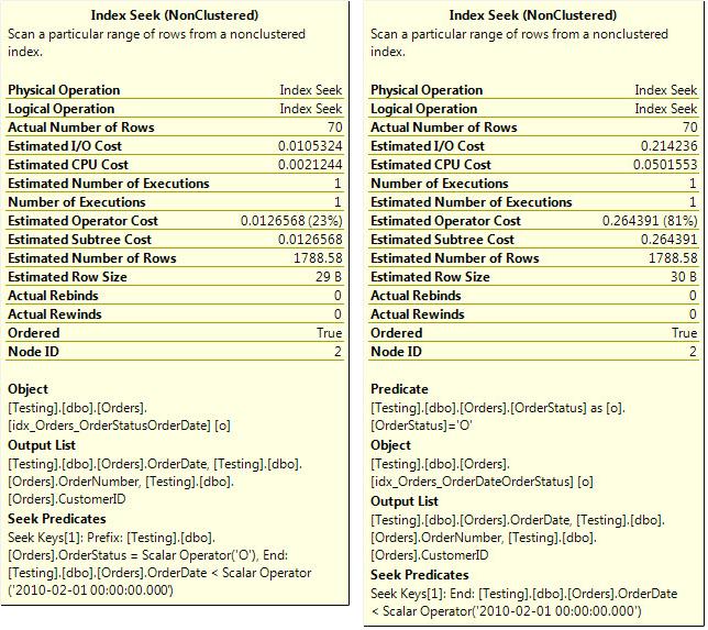
Figure 3-3. Optimal Index Seek (left) and a less-optimal Index Seek (right).

You might have noticed that the index names are different in the two displayed execution plans, and that is indeed the case. The indexes that SQL used for the two seeks were different (although the data returned was the same). That difference, although it did not result in a difference in execution plan operators that were used between the two queries, did result in a difference in performance. This difference is related to the properties shown in the Index Seek tooltips, the seek predicate (which both queries had), and the predicate (which only the not-so-optimal one had).

One thing to note, the actual row count shown in those tooltips is the number of rows that the operator output, not the number of rows that it processed. The total number of rows that the index seek actually read is not shown in the tooltip. The way to get a rough idea of that is to look at the Statistics IO and examine the logical reads (the number of pages read from memory) for the table that the index seek operates on. It’s not a perfect way to do it, but it’s usually adequate.

To understand the difference between the performance of those two queries, we need to make a brief diversion into index architecture and how index seeks work.

An index is a b-tree (balanced tree) structure with the data at the leaf level logically ordered by the index keys, as shown in Figure 3-4.

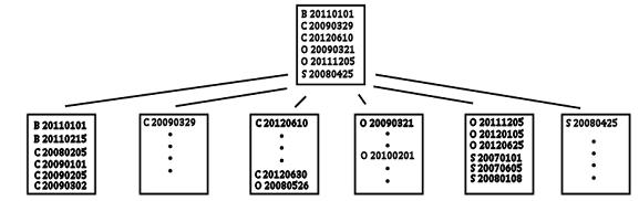
Figure 3-4. Index architecture of an index on OrderStatus, OrderDate.

An index seek operation works by navigating down the b-tree to the start (or sometimes end) of the required range and reading along the leaf level until the no more rows could possibly qualify. The seek predicate that is listed in the properties of the index seek is the condition used to locate the start (or end) of the range.

So let’s look at the two scenarios that are shown in the example.

In the first case, the optimal index seek, the seek predicate consisted of both the where clause expressions for the table. Hence, SQL was able to navigate directly to the start—or, in this particular case, the end—of the range of rows, and it was then able to read along the index leaf level until it encountered a row that no longer matched the filter. Because both of the where clause expressions on this table were used as seek predicates, every row read could be returned without further calculations being done.

In the second case, only one of the where clause expressions was used as a seek predicate. SQL again could navigate to the end of the range and read along the index leaf level until it encountered a row that no longer matched the seek predicate. However, because there was an additional filter (the one listed in the predicate section of the index seek properties), every row that was read from the index leaf had to be compared to this secondary predicate and would be returned only if it qualified for that predicate as well. This means that far more work was done in this case than for the first case.

What caused the difference? In the example, it was because the index column orders were different for the two examples.

The where clause for the query was OrderStatus = 'O' AND OrderDate < '2010/02/01'.

In the first example—the one with the optimal index seek—the index was defined on the columns OrderStatus, OrderDate. In the second example—the one with the not-so-optimal index seek—the column order was OrderDate, OrderStatus.

Let’s have another look at index architecture and see how those differ. See Figure 3-5.

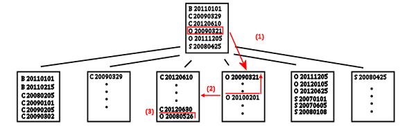
Figure 3-5. Index seek execution with an index on OrderStatus, OrderDate.

With the first index ordered by OrderStatus, OrderDate, SQL could execute the seek by navigating down the b-tree looking for the row that matched one end of that range, seeking on both columns (1). In this case, it searched for the row at the upper end, because that inequality is unbounded below. When it found that row, it could read along the leaf level of the index (2) until it encountered a row that did not match either (or both) predicates. In this case, because the inequality is unbounded below, it would be the first row that had an OrderStatus not ‘O’ (3). When that’s done, there’s no additional work required to get matching rows. That index seek read only the data that was actually required for that query.

Now, what about the other index—the one that had the columns in the other order? Take a look at Figure 3-6.

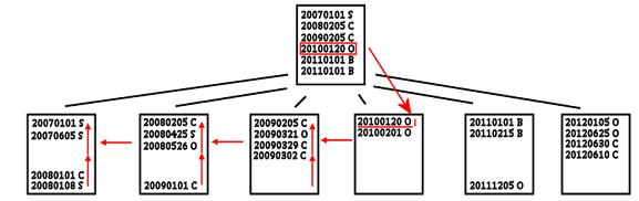
Figure 3-6. Index seek execution with an index on OrderDate, OrderStatus.

In the second case, SQL can still navigate down the b-tree looking for the row that matches one end (the upper end) of the range using both columns. This time, though, when it reads along the leaf level of the index, it can’t just read the rows that match both predicates, because the index is ordered first by the date and only within that by the OrderStatus. So all rows that match the OrderDate predicate must be read, and then a secondary filter must be applied to each row to see if it matches the OrderStatus. This secondary filter is what is shown in the tooltip as the predicate.

The reduced efficiency comes from two things. First, more rows are read than is necessary. Second, the evaluation of the filter requires computational resources. It doesn’t require a lot, but if the secondary filter has to be applied to millions of rows, that’s going to add up.

A more dramatic form of the secondary filter is when there is no where clause predicate that can be used as a seek predicate and, hence, SQL performs an index scan and applies the predicate to all rows returned from the index scan. Say, for example, I amend the earlier example and remove the where clause predicate on OrderStatus, but the only index is one with OrderStatus as the leading column. The plan for this new query is shown in Figure 3-7, along with the results.

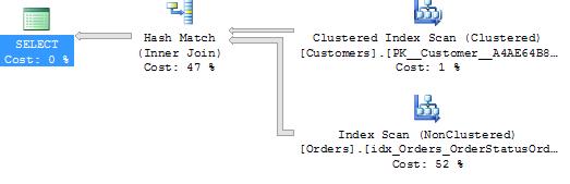
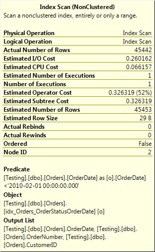
Figure 3-7. Index scan with a predicate on the OrderDate column

This results in an index scan with a predicate. (There’s no seek predicate. If it had one, it would be a seek, not a scan.) This means that every row gets read from the table and then tested against the OrderDate predicate.

So what causes this? There are a number of things. The most common are the following:

• The order of the columns in the index are not perfect for this query or necessary columns are not in the index at all.
• Any functions applied to the columns.
• Any implicit conversations.

I showed the order of the columns in the previous example. I can’t go into a full discussion of indexes here; that’s a topic large enough to need a chapter of its own. In short, SQL can use a column or set of columns for an index seek operation only if those columns are a left-based subset of the index key, as explained in a moment.

Let’s say you have a query that has a where clause of the following form:

If there is an index (for example, Col1, Col2, Col3), SQL can use that index to seek on the Col1 predicate as it is the left-most (or first) column in the index key definition. However, Col3 is not the second column, it’s the third. Hence, SQL cannot perform a seek on both Col1 and Col3. Instead, it has to seek on Col1 and execute a secondary filter on Col3. The properties of the index seek for that query would show a seek predicate on Col1 and a predicate on Col3.

Now consider if you have the same index (Col1, Col2, Col3) and a query with a where clause of the form:

Now the two columns referenced in the where clause are the two left-most columns in the index key (first and second in the index key definition) and hence SQL can seek on both columns.

For further details on index column ordering, see these two blog posts:

• http://sqlinthewild.co.za/index.php/2009/01/19/index-columns-selectivity-and-equality-predicates/
• http://sqlinthewild.co.za/index.php/2009/02/06/index-columns-selectivity-and-inequality-predicates/

There’s another form of the secondary, where one of the columns required is not even part of the index used. Let’s take this example:

Assume you have an index on SubTotal only and that the column OrderDate is not part of that index at all. SQL knows from the statistics it has that very few rows satisfy the SubTotal < 0 predicate. (Actually, none do, but there’s no constraint on the column preventing negative values. Hence, SQL cannot assume that there are no rows.) Figure 3-8 shows the execution plan for this query.

Figure 3-8. Execution plan with a seek and key lookup.

You get an index seek on the Subtotal index and a key lookup back to the clustered index, as shown in Figure 3-9.

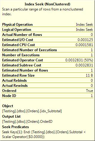
Figure 3-9. Index seek on the Subtotal index with no mention of the OrderDate predicate

The index seek has only a seek predicate. The key lookup, however, has something interesting in it. It has a predicate, as shown in Figure 3-10.

Figure 3-10. Key lookup with a predicate.

What’s happening here is that the index seek could evaluate only the SubTotal < 0 predicate because the OrderDate column was nowhere within the index. To get that column, SQL had to do key lookups back to the clustered index to fetch it. However, that column isn’t needed for output—because it’s not in the select clause—it’s needed only for the where clause predicate. Hence, each row fetched by the key lookup is filtered, within the key lookup operator, to discard any rows that don’t match the OrderDate predicate, and only rows that do match get returned from the key lookup.

Another common cause of inefficient index usage and secondary filters is the use of functions on the column in the where clause of the query. Consider the case of the table used in the example earlier, with the index on OrderStatus, OrderDate. Suppose you have an index on OrderStatus, OrderDate and the following where clause:

In other words, get all orders with a status of S that have order dates in the last month. Figure 3-11 shows the execution plan for that.

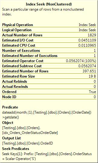
Figure 3-11. Index seek with a function resulting in a predicate.

The reason you have a predicate here and not just two seek predicates is that as soon as there is a function on the column, the where clause predicate that contains that function can no longer be used for an index seek. This is because the index is built on the column, not on function(column).

These kinds of predicates are often referred to as not being SARGable, (SARG standing for Search ARGument), a phrase that just means that the predicate cannot be used for index seek operations.

The third thing that can result in SQL having to apply secondary filters is the implicit conversion. Consider this common scenario:

The data types of the column and the parameter are different. SQL cannot compare two different data types, so one has to be converted to match the other. Which one is converted depends on the precedence rules of data types (http://msdn.microsoft.com/en-us/library/ms190309.aspx). In this case, the nvarchar data type has higher precedence than varchar, so the column must be converted to match the data type of the parameter. That query is essentially WHERE CAST(VarcharColumn AS NVARCHAR(<Column Length>) = @NVarcharParameter. That’s a function on the column. As in the previous discussion, this means that the predicate cannot be used for an index seek operation (it’s not SARGable) and can be applied only as a secondary predicate.

So, you’ve seen several causes. Now let’s look at what you can do about these.

The first thing to note is that the predicates are not always a problem. It is not always important to remove them. What is important to investigate before spending time trying to change indexes or rewrite queries is the number of rows involved. Specifically, you should determine the number of rows returned by the seek predicate and what proportion of them are then removed by the predicate.

Consider the following two scenarios: one where the seek predicate returns 100,000 rows and the predicate then eliminates 5 rows, for a total of 99,995 rows returned; and one where the seek predicate returns 100,000 rows and the predicate then removes 99,500 rows, for a total of 500 rows returned. The second scenario is a bigger problem and a bigger concern than the first.

Why? Because one of the primary goals for an index is to eliminate unnecessary rows as early as possible in the query’s execution. If a row is not needed, it is better not to read it at all rather than read it and then eliminate it with a filter. The first approach is efficient; the second approach is a waste of time and resources.

In the initial example in this chapter, the efficient option read 5 pages from the table and the inefficient option read over 300. That difference is sufficient to warrant investigation. However, if the efficient option had read 100 pages and the inefficient one had read 108, it wouldn’t be particularly worthwhile spending the time resolving the problem. You could find bigger wins elsewhere.

The first step, of course, is finding queries that have these problems. Probably the easiest way to do this is as part of regular performance tuning. Capture a workload with SQL Profiler or an extended events session, analyze it for queries doing excessive reads, and as part of the analysis see if they have inefficient index seeks.

The resolution depends on what specifically is causing the inefficient seek.

If the problem is the column order within the index, the solution is to change the order of columns in the index or create another index to fully support the query. Which option is best (and, in fact, whether either is necessary) depends on other queries that run against the particular table, the amount of data modifications that take place, the importance of the query, and how inefficient it really is. Unfortunately, a complete discussion on indexing changes is beyond the scope of this chapter.

If the cause of the inefficient seek is a function applied to a column, it’s a lot easier to resolve. Just remove the function.

Well, maybe it’s not that simple. It depends on what the function is doing as to whether it can be removed or altered.

In some cases, you can apply a function to the variable, parameter, or literal instead of the column to get the same results. An example of this is the following:

The execution plan is shown in Figure 3-12.

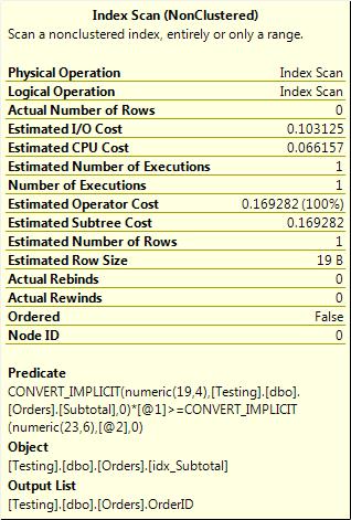
Figure 3-12. Scan caused by a function on the column in the where clause.

The multiplication that is applied to the column means that any index on Subtotal cannot be used for an index seek. If there is another predicate in the where clause, SQL might be able to seek on that and apply a secondary filter on Subtotal. Otherwise, the query has to be executed as an index scan with a secondary filter.

Basic algebra tells you that the expression x*y >= z is completely equivalent to x >= z/y (unless y is zero), so you can change that where clause to read as follows:

This example is not quite as intuitive as the first one, but it is more efficient, as Figure 3-13 shows.

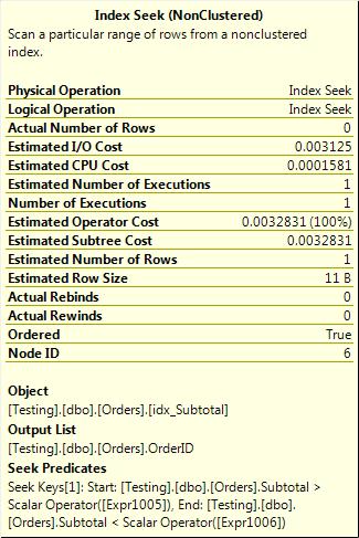
Figure 3-13. Changing where the function is evaluated results in an index seek.

Another common case is date functions, especially if a date is stored with its time in the database and the query needs to fetch all rows for a particular day. It’s common to see queries like this:

The cast to date eliminates the time portion of the datetime, so the comparison to a date returns all rows for that day. However, this is not a particularly efficient way of doing things, as you can see in Figure 3-14.

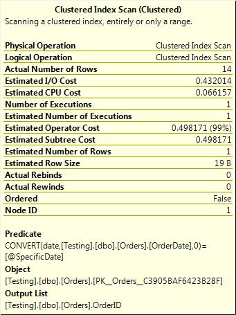
Figure 3-14. Conversion of the column to DATE results in a scan.

Instead, the query can be rewritten to use an inequality predicate and search for a range of times for the particular day, like this:

I don’t use BETWEEN because BETWEEN is inclusive on both sides and requires slightly more complex date manipulation if the rows with an OrderDate of midnight the next day are not required.

This form of the where clause is more complex, but it is also more efficient, as Figure 3-15 shows.

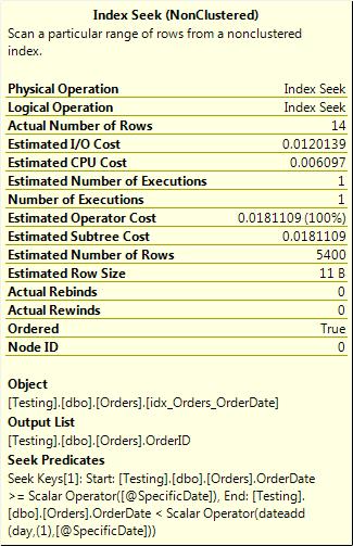
Figure 3-15. No function on the column; hence, a seek is used.

A third case is unnecessary string functions. I keep seeing code like this:

Unless the database is running a case-sensitive collation, UPPER is unnecessary (and I often see this in case-insensitive databases). RTRIM is unnecessary because SQL ignores trailing spaces when comparing strings. So ‘abc’ equals ‘abc’ when SQL does string comparisons. Otherwise, how would it compare a CHAR(4) and a CHAR(10)? LTRIM potentially has a use if the database is known to have messy data in it. My preference here is to ensure that inserts and loads always remove any leading spaces that might creep in. Then the queries that retrieve the data don’t need to worry about leading spaces and, hence, don’t need to use LTRIM.

The implicit conversion is probably the easiest problem to fix (though it’s often one of the harder ones to find). It’s mostly a case of ensuring that parameters and variables match the column types; of explicitly casting literals, variables, or parameters if necessary; and ensuring that front-end apps are passing the correct types if they are using dynamic or parameterized SQL statements.

A common culprit here is JDBC (the Java data access library), which by default sends strings through as nvarchar no matter what they really are. In some cases when dealing with this, you might need to alter the column’s data type to nvarchar just to avoid the implicit conversions if the application cannot be changed. Some ORM tools show the same default behavior.

One implication of this discussion that I need to draw particular attention to is that not all index seeks are equal, and just having an index seek in a query’s execution plan is no guarantee that the query is efficient.

I recall a discussion on a SQL forum a while back where someone was asking how to get rid of the clustered index scan that he had in his query execution plan. The pertinent portion of the query was something like this:

As mentioned earlier, the way to optimize that query is to remove the function from the column, change the where clause to use either BETWEEN or >= and < operators, and ensure that there’s a suitable index on the OrderDate column to support the query. The solution that someone posted was to add a second predicate to the where clause, specifically an inequality predicate on the primary key column (which was an integer and had the identity property with default seed and increment, and hence was always greater than 0) as such:

Does that achieve the desired goal? Figure 3-16 has part of the answer.

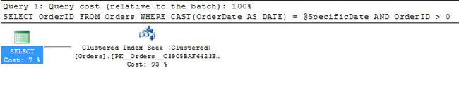
Figure 3-16. Clustered index seek.

It seems to achieve the desired goal because there’s a clustered index seek now. But what’s that seek actually doing? See Figure 3-17.

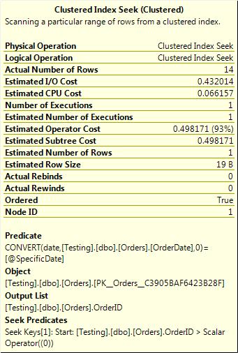
Figure 3-17. Very inefficient clustered index seek.

The seek predicate OrderID  > 0 matches every single row of the table. It’s not eliminating anything. (If it did, adding it would change the meaning of the query, which would be bad anyway.) The predicate is the same as it was before on the index scan. It’s still being applied to every row returned from the seek (which is every row in the table), so it’s just as inefficient as the query was before adding the OrderID > 0 predicate to the where clause. An examination of the output of statistics IO (which I will leave as an exercise to the reader) will show that adding that OrderID > 0 predicate made no improvements to the efficiency of the query.

Be aware, not all index seeks are created equal and adding predicates to a where clause just so that the execution plan shows a seek rather than a scan is unlikely to do anything but require extra typing.

Residuals

Moving on to residuals, they are similar in concept to the predicates on index seeks, index scans, and key lookups, but they are found in a different place. They’re found on joins, mainly on merge and hash joins. (Residuals on a loop join usually show up as predicates on the inner or outer table, or sometimes both.)

Let’s start with an example:

The plan for this query is shown in Figure 3-18.

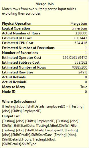
Figure 3-18. Partial join.

The tooltip of the join operator shows that the Join columns was EmployeeID only. There’s no mention of my date expression. Where did that go? See Figure 3-19 for the answer. It shows that it went into the join residual section in the properties of the join operator.

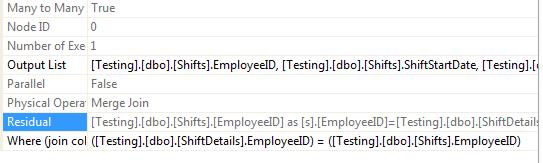
Figure 3-19. Join residual as seen in the properties of the join operator.

It’s hard to see what’s happening there, so I repeated it and cleaned it up here:

The join columns just contains the EmployeeID; it’s the residual that has both. What’s happening here is that SQL evaluates the join on the join columns (in this case, EmployeeID) and then applies the filter listed in the residual to every row that qualifies for the join. If the match on just the join columns isn’t very restrictive, you can end up with a huge intermediate result set (a partial cross join, technically) that SQL has to find memory for and has to work through and apply the residual to. This can be seen in the properties of the join, as shown in Figure 3-20.

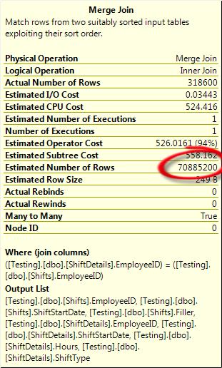
Figure 3-20. Many-to-many join with a huge row count.

There are 70 million rows estimated, and that’s estimated based on what SQL knows of the uniqueness of the join columns on each side of the join (and in this case, the EmployeeID is not very unique in either table). The Actual Row Count (as mentioned earlier) is the total rows that the operator output, not the total rows that the join had to work over. In this case, the number of rows that the join operator had to process is a lot higher than the number that were output (probably close to the estimated rows).

Depending on how many rows match on just the join columns (vs. both the join and the residual), this can result in minor overhead or major overhead.

To put things in perspective, the prior example ran for 14 minutes. A fixed version that joined on a direct equality on both EmployeeID and ShiftStartDate and had both predicates listed in the join columns (and returned the same rows) ran in 20 seconds.

Hash joins can also have residuals. The properties of the hash join (shown in Figure 3-21) show the join and the residual slightly differently to the merge.

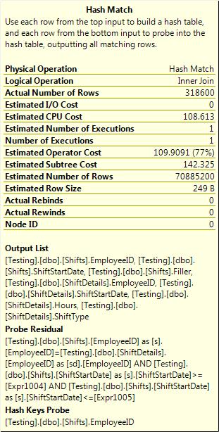
Figure 3-21. Hash join properties.

The columns that are used to join appear as Hash Keys Probe in the tooltip, and as Hash Keys Build and Hash Keys Probe in the properties of the join operator (as shown in Figure 3-22). The columns for the residual appear in the probe residual in both the tooltip and the properties.

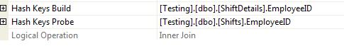
Figure 3-22. Hash join build and probe columns.

As with the merge join, the number of rows that the residual has to process affects just how bad it will be in terms of performance.

That’s all well and good, but how do you fix them?

As with the predicates on index seeks and scans, multiple things can cause residuals.

Unlike predicates, the index column order is not a main cause. Hash joins don’t mind the index column order much. Merge joins do because they need both sides of the join to be sorted on the join columns, and indexes do provide an order. However, if the order isn’t as the merge wants it, the optimizer can put a sort into the plan or it can use a different join, such as a hash join.

Mismatched data types can result in joins that have residuals, as Figure 3-23 shows. By “mismatched data type,” I mean joins where the two columns involved are of different data types. The most common ones I’ve seen in systems are varchar and nvarchar, varchar and date, and varchar and int.

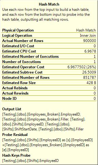
Figure 3-23. Hash join with a residual caused by a data type mismatch.

It’s not clear from the tooltip shown in Figure 3-23 that any conversions are occurring; even the properties do not show anything wrong. In fact, the presence of the residual is the only hint that something’s not right. If you compare that to a query where the data types do match (shown in Figure 3-24), you’ll notice that there’s no residual in that case.

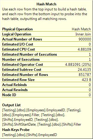
Figure 3-24. Hash join without a residual.

The last cause I’ll look at is strange join predicates. By “strange,” I mean something like an inequality in the join predicate.

Merge joins and hash joins are both limited to being able to use equality predicates only for the actual join. Anything other than an equality has to be processed as a residual. (Nested loop joins do not have such a limitation.) This was the example I used initially: a join with a between because the date in one table was a date with the time set to midnight, and the date in the other table had a date with a time other than midnight. Hence, the only way to join those was with a between, and that resulted in the inefficient join.

Mismatched data types and non-equality join predicates are often indications of underlying database design problems—not always, but often. Fixing them can be difficult and time consuming. In the case of the mismatched data types, fixing the problem might require altering the data type of one or more columns in a database, or possibly even adding additional columns (usually computed columns) that convert the join column to the matching data type for an efficient join.

Queries that join on inequalities are harder to fix. Although there are certainly legitimate reasons for such a join, they should not be common. The fixes for queries using inequality joins depend very much on the underlying database and how much (if at all) it can be modified.

The example I started the section with has a Shifts table with a ShiftStartDate that always contains a datetime where the date portion is midnight and a ShiftDetails table with a ShiftStartDate that has dates with time portions that are not midnight, and the join needs to be on the date. To optimize that query and to avoid the inequality join predicate you could add another column to the ShiftDetails table that stores the date only. This would likely be a persisted computed column. Of course, that assumes the application using those tables won’t break if another column is added.

Fixing these kinds of problems in an existing system is very difficult and, in many cases, is not possible. It is far better to get a correct design up front with appropriate data type usage and properly normalized tables.

Spills

The third form of hidden performance problem that I want to discuss is the spill. Before I can explain what a spill is, I need to briefly explain what memory grants are.

A memory grant is an amount of memory that the query processor will request before it starts executing the query. It’s additional memory that the query needs for things like hashes and sorts. The memory grant amount is based on the number of memory-requiring operations, on whether or not the query will be executed in parallel, and on the cardinality estimates in the execution plan.

I don’t want to go too deep into the process of requesting and granting that memory; it’s not essential for the rest of this section. If you are interested in the topic, you can refer to the following blog entries for further detail: http://blogs.msdn.com/b/sqlqueryprocessing/archive/2010/02/16/understanding-sql-server-memory-grant.aspx and http://www.sqlskills.com/blogs/joe/post/e2809cMemoryGrantInfoe2809d-Execution-Plan-Statistics.aspx. Also, you can view the presentation that Adam Machanic did at the Pass Summit in 2011 (http://www.youtube.com/watch?v=j5YGdIk3DXw)

The use of memory grants is all well and good, but those memory grants are based on cardinality estimates and estimates can be wrong. So what happens when they are wrong?

Let’s compare two examples, one with an accurate estimate and one with a badly inaccurate one. (I’ll use some hints to force a bad estimate because it’s both easier and more repeatable than creating actual stale statistics or simulating other conditions that result in poor estimates.)

The two plans look identical, so I’m not going to show them (two index seeks, a hash join, and a select). I’ll just show the properties of the hash joins and of the selects for the two.

The first query, with accurate estimations, is shown in Figure 3-25.

The second query, with poor estimations, is shown in Figure 3-26.

Ignore “Estimated Number of Rows 1” on the tooltip of the select. That shows up because the outer select was a COUNT (*).

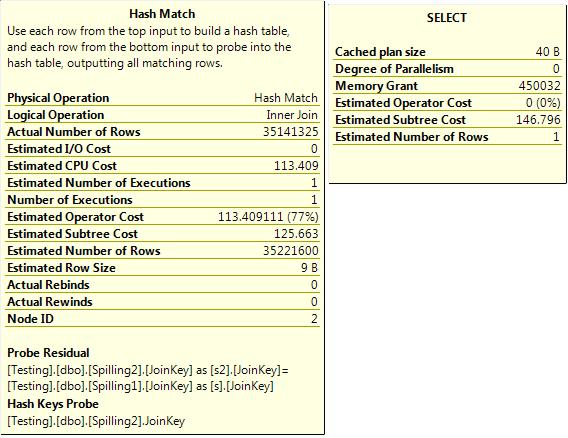
Figure 3-25. Accurate estimations.

If you take a look at those, the first hash join has an estimated row count of 35 million and an actual row count of 35 million. To do the hash join (which was a many-to-many join), the query was granted 450 MB of workspace memory.

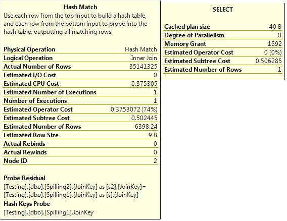
Figure 3-26. Inaccurate estimates.

The second query has an estimated row count of 6,000 rows and an actual row count of 35 million. The memory grant that the query execution engine requested was based on that estimate, and was 1.5 MB. If the first query required 450 MB to do the hash join, the second is not going to be able to do it in 1.5 MB. So what happens? Figure 3-27 shows the result.

A hash spill happens. I won’t go into the complexities of hash spills here because that’s beyond the scope of this chapter, but in short, portions of the hash table are written to TempDB and then read back when necessary. This can happen once or it can happen repeatedly during the execution of the query.

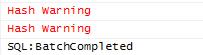
Figure 3-27. Hash warnings viewed via SQL Profiler.

As I’m sure you can imagine, that’s not going to be good for performance. Memory is many times faster than disk and having to write and re-read portions of what should be an in-memory structure is going to make the query run slower than it otherwise would. In this example, the query that didn’t spill took on average 8 seconds to run and the query that did spill took on average 10 seconds. That’s not a huge difference, but that was on a machine with a single user and no other appreciable I/O load.

In addition to the hash spill, there are other operations that can spill—sorts and exchanges being the most common. Spools also use TempDB, but that’s not so much a spill as the fact that a spool is, by definition, a temporary structure in TempDB.

The obvious outstanding questions are how do you detect these spills, what do you do about them, and how do you prevent them?

Detecting hash spills is the easy part. There are three SQLTrace events that fire in response to hash spills, sort spills, and exchange spills. They are hash warnings, sort warnings, and exchange warnings, respectively.

Those trace events show only that a spill has happened; they don’t say anything about how much data was spilled to TempDB. To detect that information, you need to turn to the Dynamic Management Views—specifically, to sys.dm_db_task_space_usage and sys.dm_db_session_space_usage. I’ll use the second one because it is a little easier. The first one shows data only for currently executing queries. The second one shows data for currently connected sessions.

This query tells you how much space in TempDB any current connection has used, along with either the currently running command or the last command that was run.

Using that on the earlier example, I can see that the query that didn’t spill had 0 pages allocated in TempDB. The query that did spill had 0 pages of user objects and 10,500 pages of internal objects—that’s 82 MB. (A page is 8 KB.)

That query can be scheduled to check for any processes that are using large amounts of TempDB space and to log any excessive usage for further investigation. Large amounts of internal allocations don’t necessarily indicate spills, but it’s probably worth investigating such readings. (Large amounts of user allocations suggests temp table overuse.)

On the subject of fixing spills, the first and most important point is that spills cannot always be prevented. Some operations will spill no matter what. A sort operation is the poster child here. If you imagine a sort of a 50-GB result set on a server with only 32 GB of memory, it’s obvious that the sort cannot be done entirely in memory and will have to spill to TempDB.

Tuning spills has three major aspects:

• Prevent unnecessary spills caused by memory grant misestimates.
• Minimize the number of operations that have to spill.
• Tune TempDB to be able to handle the spills that do happen.

Memory grant underestimates are often a result of row cardinality misestimates. These can be caused by stale statistics, missing statistics, non-SARGable predicates (as discussed in the first section of this chapter), or a few less common causes.

For more details on cardinality problems, see the following:

• http://blogs.msdn.com/b/bartd/archive/2011/01/25/query_5f00_tuning_5f00_key_5f00_terms.aspx
• http://msdn.microsoft.com/en-us/library/ms181034.aspx
• Microsoft SQL Server 2008 Internals by Kalen Delaney (Microsoft Press, 2009)

Minimizing the number of operations that have to spill is mostly a matter of application design. The main points are not to return more data than necessary and not to sort unless necessary.

It’s common for applications to fetch far more data than any user would ever read, retrieving millions of rows into a data set or producing a report with tens or even hundreds of pages of data. This is not just a waste of network resources and a strain on the client machine, but it can often also lead to huge joins and sorts on the SQL Server instance.

There’s a fine line between a chatty application that calls the SQL Server instance too many times requesting tiny amounts of information and an application that fetches far too much data, wasting server and client resources.

When you are designing applications, it is generally a good idea to fetch all the data for a particular screen or page in the smallest number of calls possible. That said, don’t err on the side of fetching the entire database. The user should be able to specify filters and limitations that restrict the data that is requested. Don’t pull a million rows to the app and let the user search within that. Specify the search in the database call, and return only the data that the user is interested in.

On the subject of sorts, note that it’s worthless to sort the result set in SQL Server if the application is going to sort it when displayed. It’s also sometimes more efficient to sort the result set at the client rather than on the server, because the client is dealing only with the one user’s requests and small amounts of data while the server is dealing with multiple concurrent requests. You should consider this during the application design and development phases. It’s certainly not always possible to do this, but you should at least consider whether it can be done.

The last part is tuning TempDB for the cases that will spill. This is one of those areas where almost everyone has an opinion and none of them are the same. I won’t go into huge amounts of detail; rather, I’ll just give you some solid guidelines.

Unless you have a storage area network (SAN) large enough and configured to absorb the I/O requirements of TempDB and the user databases without degradation, the TempDB database should preferably be placed on a separate I/O channel from the user databases. This means putting them on separate physical drives, not on a partition on the same drive as the user databases. Preferably, you should use a dedicated RAID array.

TempDB should be on a RAID 10 array if at all possible. If not, RAID 1 might be adequate. RAID 5 is a bad choice for TempDB because it has slower writes than RAID 1 or 10 because of the computation of the parity stripe.

I’ve heard of suggestions to use RAID 0 for TempDB. In my opinion, this is a very dangerous suggestion. It is true that there is no persistent data in TempDB (or at least there shouldn’t be) and, hence, losing anything in TempDB is not a large concern. However, RAID 0 has no redundancy; if a single drive in the array fails, the entire array goes offline. If the drive hosting TempDB fails, SQL Server will shut down and cannot be restarted until the drive is replaced or TempDB is moved elsewhere. Hence, although using RAID 0 for TempDB does not pose a risk of data loss, it does have downtime risk. Depending on the application, that might be worse for the app.

If Solid State Drives (SSD) are available, putting TempDB onto the SSD array should be considered—just considered, not used as an automatic rule. It might be that a user database has higher I/O latency than TempDB and would hence benefit more, but it is definitely worth considering and investigating putting TempDB onto an SSD array if one is available.

On the subject of the number of files for TempDB, much has been written. Some writers on the topic even agree.

There are two reasons for splitting TempDB into multiple files:

• I/O throughput
• Allocation contention

Allocation contention seems more common than I/O throughput, though it isn’t clear whether that’s just because it’s talked about more or whether it occurs more. Allocation contention refers to frequent PageLatch waits (not PageIOLatch) seen on the allocation pages in TempDB, usually on page 3 in file 1 (appearing as 2:1:3). They also appear on page 1 and 2 (appearing as 2:1:1 and 2:1:2), though those are less common. These waits can be seen in sys.dm_exec_requests or sys.dm_os_waiting_tasks.

The contention happens because (very simplified) anything writing to TempDB needs to check those pages to find a page to allocate and then needs to update that page to indicate that the allocation has been done. The primary solution for allocation contention is to add more files to TempDB. How many, well, that depends. You can read more about this at the following website: http://www.sqlskills.com/BLOGS/PAUL/post/A-SQL-Server-DBA-myth-a-day-%281230%29-tempdb-should-always-have-one-data-file-per-processor-core.aspx.

Splitting for I/O throughput is less common. If the dedicated array that holds TempDB is not providing adequate I/O throughput and cannot be tuned, you might need to split TempDB over multiple dedicated arrays. This is far less common than splitting for allocation contention.

For further reading, see the white paper “Working with TempDB in SQL Server 2005” (http://www.microsoft.com/technet/prodtechnol/sql/2005/workingwithtempdb.mspx).

Conclusion

All of the problems looked at in this chapter are subtle, hard to see, and very easy to miss, especially in the semi-controlled chaos that many of us seem to work in these days. I hope the details I provided give you valuable insight into some design and development choices that can influence the performance of your apps and systems in various ways. This chapter also described additional tools and processes you can examine and experiment with when faced with performance problems.