CHAPTER 18
![]()
Tuning for Peak Load
Today is historically the busiest day of the year for your online shopping business. At 11 AM, the system is starting to show signs of strain and load that exceeds that of the previous year. Customers are having problems completing their orders. Some fail, others are just slow. The operations center calls you in to see what’s going on with SQL Server, and you observe that processes are starting to queue up because of large blocking chains, which ultimately affects the checkout process. You didn’t code the application, but your job as a database administrator (DBA) is to fix the problem. As this event is unfolding, upper management is concerned and the Chief Information Officer (CIO) is standing over your shoulder watching you try to resolve the issue—no pressure there. Things eventually calm down later in the day, but it is unknown how many sales or potential customers were lost because of the slowdown or failed checkouts. In addition to the orders being affected, replication to the reporting environment now has 12 hours of latency affecting the reports to internal consumers of the raw sales data. Can you prevent this scenario from happening? In many cases, you can.
Every organization has mission-critical applications that run the business. These applications must scale and perform to handle load when the system is at its busiest—otherwise known as its peak load. Peak loads might occur daily or at varying intervals, often during the peak season; it’s not necessarily just a once-a-year occurrence such as the holiday season (which could be considered a peak season) described in the preceding example. To address these challenges, organizations must plan for these events well in advance so that they can have peace of mind that their systems will meet the increased traffic demands. Failure or downtime is often not an option because most businesses either depend on a large percentage of revenue from these peak times or have mission-critical business events, such as an accounting department’s year-end close.
The way your solution looks the day it is put in place is not the way it will look 10, 100, or 1,000 days later. More users are added and traffic increases. You need to anticipate the change not only in daily usage (which might represent your peak time), but also for those special times when system performance is crucial. This chapter will show you how to plan for the times when your servers will need to scale and perform to handle this additional traffic.
Define the Peak Load
Do you know how many transactions you expect during the peak hour of your peak day? If so, how accurate is that number? Are there documented performance requirements for the core transactions to meet the service level agreements (SLA)? Have you measured how many transactions the current system can handle day to day? These and many other questions are important to answer before the business can feel comfortable about going into the peak season.
Every application and environment is different. However, there is one thing that is constant: no single action will make the system scale. A combination of different things must happen to achieve the desired result. For example, the business cannot assume that purchasing newer, bigger hardware will solve its performance woes and make the application scale. Think about your critical application and how a large blocking chain during the core business hours might affect the application and, ultimately, the business itself. Hardware will not account for, nor fix, blocked internal resources in SQL Server. Blocked resources is an application issue, even if it winds up being as simple as fixing an index or something as complex as rewriting application logic. The process to prepare the application for the peak load is a repetitive one that often must be repeated several times before the environment is ready to scale to meet the additional load.
Before you can do any analysis to possibly remediate the application to handle your peak load, you need to put a multifunctional project team in place. The project team should consist of various groups from across the enterprise, including the technical and nontechnical sides of the business.
Here is the makeup of a typical project team, listed by function:
- Project manager
- Several application representatives
- DBA lead
- Storage resource
- Network resource
- Server resource
- Business representative
The project team’s major responsibility is to clearly define the goals that must be met during the peak usage time (whether it’s an event, day-to-day use, seasonal use, and so forth) and to implement the changes necessary to enable the systems to meet or exceed these goals. These goals must be formally documented and agreed upon so that everyone is on the same page when it comes to expectations. If this is not done, you might wind up in the scenario that started the chapter.
Start by defining what is expected during the peak window. Depending on the environment and the company, this exercise might be easier for you than others. The expectation should always start as a nontechnical requirement from the business. Discussions to get to that expectation often involve looking at the current market conditions and reviewing a lot of data, both current and historical. The goal is to define how many business transactions the company expects to process within a certain period of time. The transactions represent the core processes the consumer or end user will use or initiate during the peak season. For example, if your company is an online retailer, the core transactions might be product searches, adding products to the shopping cart, the checkout process, processing payments, and reviewing orders. What you’re really trying to understand is this: when will the transactions occur, and what is the expected peak volume? How many orders does the company anticipate confirming within an hour or day? Is it 1,000 per hour or 500,000 per day? Does that volume change at certain times of the day, month, or year? Planning for 1,000 transactions per hour is very different than planning for a workload of 500,000 transactions. You need to design solutions to meet the maximum number of transactions during the peak time frame.
Applications are the key, so mapping something like X sales per hour to the number of transactions in the system to how many transactions need to occur in SQL Server is important. This gives the technical side of the team an idea of where to start and what to look for and architect to.
The number of business processes that are expected during the peak season or peak hours is not the only measurement you need to determine. How long can the average response time be? The response time should meet the expectations of end users regarding how long the end-to-end transaction should take. Most of us can design a system to process a high number of transactions, but it is another task entirely to guarantee the transactions are completed within a specific time frame. This is often specified in the performance-based SLA you will be measured against. Even if it hasn’t been formally documented, the SLA often has already been defined for the core business processes. The performance SLA is one of the most important factors to the business and the customer because if you do not fulfill the terms of the contract, there are different ramifications, including financial penalties. For example, the credit card industry often specifies in an SLA a response time of two seconds to perform a balance check. If the response does not come back in a certain amount of time, the company on the other side of the transaction might have to stand in for the transaction. For each stand-in, there is a cost and these costs can add up fast. If the system is not available for 10 minutes on a big retail shopping day like Black Friday in the United States, it could cost a company several hundred thousand dollars.
Defining what is transactional volume during the peak load is often one of the most crucial and challenging tasks for the business to do. If the business misses the mark with regard to implementing appropriate response times, it might not have enough resources to process all of the transactions or might even end up seeing its systems fail because there is not enough capacity. Having excess capacity can be a good thing to account for unforeseen growth, and a good rule of thumb is to add 20 percent to the peak numbers. What you want to avoid is having too much capacity, which means that the business might have spent money unnecessarily. At the end of the day, there is a balance that must be achieved.
Once you have the formalized requirements, the technical team has to take the business requirements and map them to technical requirements, which is a vastly different exercise.
Determine Where You Are Today
Preparing a system for the peak load is like training for a marathon and not getting winded by running a sprint. Once the team sets the formal expectations, you have to analyze whether you can handle your peak load. This is not a straightforward process. To begin, you must put together a list of the applications, servers, instances, databases, and so forth that are affected by the peak-load requirement. For example, in a larger organization, the peak season might involve or touch numerous individual servers, with each one being impacted by the additional load in different ways. For smaller organizations, it might involve a handful of web servers and a single server running SQL Server. Just because there are fewer servers does not necessarily mean it is easier to plan for your peak usage. It depends on what is being asked for when it comes to performance.
You must assess each application and its associated back end to see where you are today versus where you need to be to meet the peak load. An important part of this effort is to discover the environmental constraints, including items that cannot be changed or addressed in the short (or long) term. These environmental constraints need to be identified early on so that a workaround can be planned if necessary, because additional lead time is often needed to address them. Some of the most common limitations are application editions or versions; infrastructure like storage area network (SAN) capacity or performance; and server hardware, such as a motherboard that cannot support additional memory. These constraints are important to know up front because they need to be in the back of your head when you are assessing the environment.
If the environment you support is large and includes many systems that make up the core business, you should prioritize the applications and their associated servers into Tier 1 and Tier 2. The Tier 1 applications initiate and support the core business processes. To determine if an application is Tier 1, ask yourself this question: If the application or its servers are not up, can a transaction be completed? If the answer is no, it is a Tier 1 application. Tier 2 applications provide auxiliary functions and are not required to be up and performing to complete a core transaction. Reporting servers are often classified as Tier 2 because processing the sales transaction is more important than providing a report on how many products were sold. By classifying each application in this way, you will have a smaller list of applications to perform the initial assessment on, which is important if the timeline is tight.
![]() Note Because this book is focused on SQL Server, I’ll concentrate on assessing each application from the viewpoint of using SQL Server. Your assessment should also take into account other aspects such as infrastructure, the underlying server hardware, and Windows. Everything matters.
Note Because this book is focused on SQL Server, I’ll concentrate on assessing each application from the viewpoint of using SQL Server. Your assessment should also take into account other aspects such as infrastructure, the underlying server hardware, and Windows. Everything matters.
For the purposes of this chapter, the following scenario will be used:
- The application is an online tax application that allows users to enter their federal tax information online with a workflow to assist them, save the tax return, file the forms online with the federal government, and process the payment.
- Historically, the application has had performance issues during the tax season, specifically with reporting and with some of the payment processes.
- A dedicated environment does not exist for performance testing. All performance and system testing is done in the Quality Assurance (QA) department, which is half the size of the production environment but shares the same type of disk subsystem.
- The growth rate for the number of returns processed online and the number of payments processed is shown in Table 18-1.
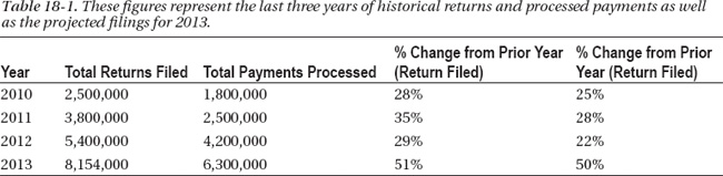
![]() Note Assume that new functionality is being released in the program, which is being heavily marketed. Because of these factors, it is estimated the application will see a 22 percent increase in filings in 2012.
Note Assume that new functionality is being released in the program, which is being heavily marketed. Because of these factors, it is estimated the application will see a 22 percent increase in filings in 2012.
As shown in Figure 18-1, this physical environment consists of three web servers running Internet Information Services (IIS), two middle-tier servers, and a single SQL Server cluster running SQL Server Standard Edition 2012, which hosts three databases that consume 900 GB. The application is a .NET application and leverages the middle tier for all data access, connection management, transaction management, and session state. The database has the basic maintenance processes in place and is supported by a part-time DBA.
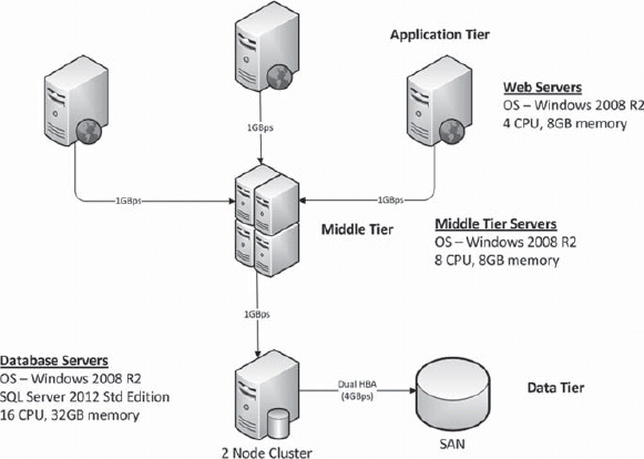
Figure 18-1. A high-level topology diagram for the tax application.
Perform the Assessment
Where do you start to figure out what is going on—especially in a large environment? You need a road map, and creating one is facilitated by identifying existing sources of data within your environment. Check to see if a topology diagram or configuration management database (CMDB) repository exists. The topology diagram will provide the 50,000-foot view of the application. Depending on the level of information maintained in the CMDB, you might be able to see the server details, application owners, as well as application relationships—all of which are important when working with a system you might not be familiar with. The goal is to identify any other applications the primary application might interface with because it might impact the scalability.
If a CMDB does not exist in your environment, work with the server, operating system (OS), and storage teams to gather the basic configuration information about the application environment. Table 18-2 contains a high-level list of important attributes to collect from each server. What if you do not know what a lot of the information in Table 18-2 means? This is why you put together a multidisciplined project team with members from all areas of technology that will be responsible not only for gathering this data, but for working with you to analyze the data. The goal of the project team is to bring together all of the data, analyze it, and determine what needs to be addressed based on the goals the business has defined.
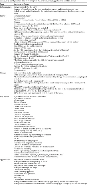
Configuration data by itself is useful, but often it needs to be paired with performance-based runtime information to create the full picture. The configuration data in Table 18-2 will be used later, after you have collected additional application data, additional runtime data, and historical performance data. The data gathered often leads to other questions, other data that will be captured, and ultimately, other conclusions.
Define the Data to Capture
After you have the base information about the environment, you can collect performance data. Depending on your environment, some or all of the performance data might already exist in some format that you and your team members can access without a lot of extra effort. Most environments have some level of monitoring in place already, which generates alerts based on certain conditions and also stores the performance metrics for a period of time. Historical performance information is a treasure trove of information if it is available because the data can be analyzed to establish trends over time. The farther back you can go, the more trends you can see. If you are lucky, you might have captured the performance data from the last peak time frame. If any of this type of data does exist, be sure to use it, back it up, and save it for future analysis. This type of information is valuable because most products archive or aggregate older data, which results in a loss of data fidelity.
Collecting System Performance Data
Whether or not you already have performance data for the application and database servers, SAN, and network, you still need to have current information. More importantly, you need to have the right items captured. Capturing information for the sake of capturing information is a pointless exercise. This effort does not need to cost a lot of money or take a lot of work to put in place. Several tools are available that capture performance data. If you do not have money in the budget to purchase them, you can leverage native tools that Microsoft provides for free. You can use Performance Monitor (often referred to as just Perfmon), which is built into Windows, to collect hundreds of performance metrics with very little overhead. Perfmon allows users to create a data collector, which is a saved profile that contains a list of the objects to capture, the file location for the data, the format of the file, the start and end times, and the interval, which can be measured down to the second. Remember, though, that just because it can capture data every second does not mean you should—or could—do it. (For example, collecting data this frequently might add unnecessary overhead, depending on how much data you are capturing.) You need to think about the goal of your data collector and how frequently you need the data to be collected to meet that goal.
What to capture will depend on the application as well as what technologies your application is using. For SQL Server and the related server-level data, the goal of the collection process is to capture information related to the processor, the network, the disk, memory, and SQL Server itself. The goal of the data capture is to identify if there is any pressure within a certain layer. If there is, you should capture additional information to understand why that is happening. The secondary goal of the data capture is to be able to use this data as a performance baseline.
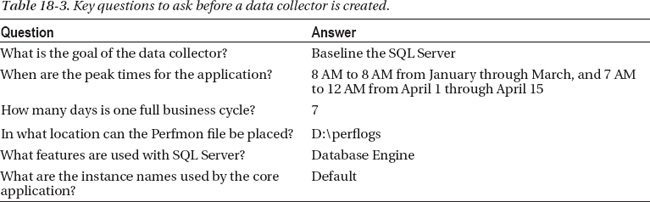
Now that you understand the goals, I’ll apply the data-capture principles just described to an example scenario. Before you can start a process like this, you need to answer some questions that will drive the data-collector configuration. An example of what types of questions you need to answer is shown in Table 18-3. Without having answers to these questions, the data collector might not collect data for the core business hours or the right features. If the peak window times are not captured, you will end up with misleading data to analyze.
Using the answers just shown, follow these steps to create a new data collector set in Perfmon:
- To open Perfmon, click on Start Administrative Tools and select Performance Monitor.
- When Perfmon is open, expand Data Collector Sets. Right-click User Defined, and select New from the context menu.
- The dialog box shown in Figure 18-2 appears. This is where you have a choice to make. If you are new to Perfmon, you might want to choose Create From A Template so that you can use predefined options. After you have worked with Perfmon a few times, choosing Create Manually is the way to go. The manual mode allows you to create a data collector that is customized to the situation. Make your choice, and click Next.
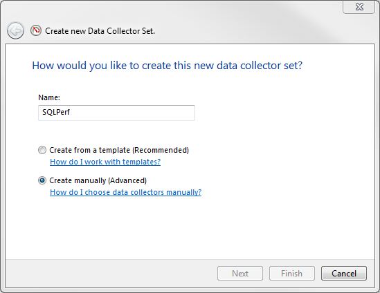
Figure 18-2. Creating a manual data collector.
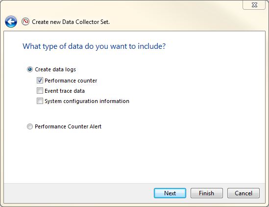
- The next step is to define what type of data you will collect (as shown in Figure 18-3). Normally, you will choose Performance Counter because you can use this option to collect the performance data from the system. However, as you can see, there are other options in the dialog box you can use to capture more data about a server.
- After you select Performance Counter and click Next, you need to select the objects you want to capture (as shown in Figure 18-4). There are many options, which can be daunting. Before you choose any objects, think back to the core areas of the system: CPU, network, disk, memory, and SQL Server. The goal is to capture high-level data for each of these areas. For the scenario defined earlier, the counters defined in Table 18-4 will be used. You can use this configuration as a starting point for any system where you want to gain high-level insight into how busy the system is, the system’s health, and the system’s pain points.
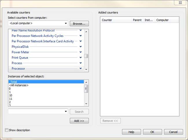
Figure 18-4. Displays the objects that can be selected for monitoring SQL Server, Windows and many other applications
Note SQL Server dynamic management views (DMV) can provide additional data for many of the SQL Server–related Performance Monitor counters. If an object counter records a level that is above a certain threshold and additional information is required, consider using DMVs to provide a better picture of the situation.
- The last step is to schedule the data collector. Click on the Schedule tab, as shown in Figure 18-5. This tab provides several options for scheduling, such as Beginning Date and Expiration Date, along with options for specifying the time and days. You can use the options on this tab to schedule the data collector over a weekend or during off-peak hours. To add a schedule, Click on the Add button and select the beginning date and Expiration Date.
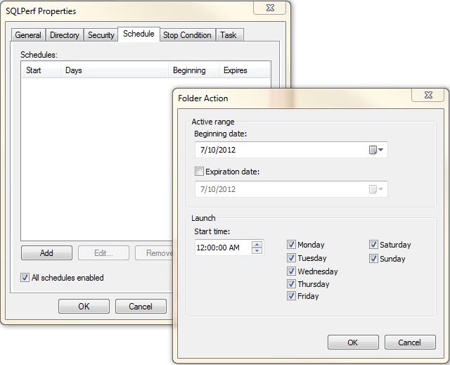
Figure 18-5. The Folder Action dialog box, which was accessed from the Schedule tab, for a data collector.
- Another tab that is commonly used is Stop Condition, which is shown in Figure 18-6. You can use this tab to define stop conditions for the data collector. This is important because you can use it to ensure that the data collector does not run for an extended period of time and eventually cause additional issues on the system. A common rule to follow is to always define a stop condition based on time or file size. This minimizes the risk that the data collector will fill up the system partition and cause an outage.
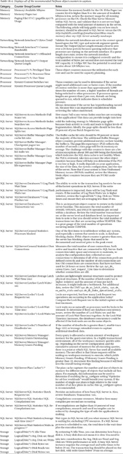
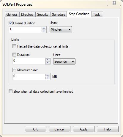
Figure 18-6. The Stop Condition tab for a data collector.
Collecting Application Performance Data
The Perfmon data collected to date provides a view into how the servers themselves are performing, but it is only one view of what is going on. This information does not tell you what type of code SQL Server is running, what type of calls are being executed from the various application servers, and whether the performance is optimal. Capturing this type of data is called application profiling. Application profiling involves capturing all of the application calls generated by performing a single action from a process or an end-user request. Profiling an application gives you important data related to performance tuning an application. This information helps you understand what operations the application is performing for a specific request. Following are several questions to get answers to when you are reviewing the application profile data.
![]() Note These application-profile questions are focused on the database tier.
Note These application-profile questions are focused on the database tier.
- How many database statements were executed for each request?
- Were the database statements part of a single batch, or is each one a separate database call?
- Is the application using connection pooling? If not, how many loginlogouts occurred for each application request?
- Are the database calls ad-hoc or stored procedures?
- Are there statements that consume a high number of physical resources—such as CPU or I/O—or are there long-running statements?
To profile an application, you can use SQL Server Extended Events to define custom traces to capture the application requests and other pertinent data. Just like the Perfmon data, this data can be used as a baseline for the application or the database server.
![]() Note SQL Server Profiler was deprecated as of SQL Server 2012, so it is recommended you start learning how to use the Extended Events feature.
Note SQL Server Profiler was deprecated as of SQL Server 2012, so it is recommended you start learning how to use the Extended Events feature.
Before you can start, you need to define the different types of data you want to capture. Typically, there are four types of traces that are run to capture different types of data, as shown in Table 18-5, with some sample guidelines.
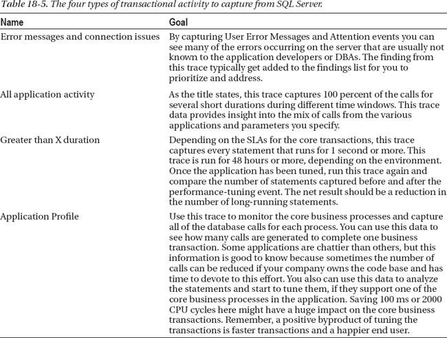
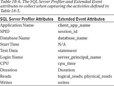
When using Profiler to capture system activity, make sure to create a server-side trace and log the information to a file locally. If possible, save the file to a faster drive (especially one that does not contain the data and log files for the database being analyzed) to improve the performance. Table 18-6 is a list of recommend columns to capture when you use Profiler or Extended Events.
Analyze the Data
By now, you have collected a large amount of data, which might include topology diagrams, configuration information about the servers and applications, runtime data from SQL Server, and performance data from the network, servers, and applications. This information represents the current state of the environment, and you need to analyze it from the top down to fully understand the application and identify potential areas to address related to the business goals.
Analyzing Application-Usage Data
One of the important questions you asked the business to provide was related to the usage and performance metrics for the core business transactions that need to scale. This usage data, when coupled with the system metrics, provides you with valuable insight into what state the system is currently in. This is important because if you don’t know what state the system is in (and what state it has been in recently), it is impossible to plan for the future. When it comes right down to it, this is a capacity-planning exercise. The goal of this specific capacity-planning exercise is to create a mental picture about the application to fully understand the why, when, what, and where of the configuration options, processes, and timing of events. You need to know this to determine how many business transactions the application can support for a specific configuration.
Figure 18-7 shows an example of performance data collected from a third-party monitoring tool. It shows the cumulative number of requests and the response time by day for a two-month period. The Latency (measured in ms) is on the left axis, and the total number of requests are shown on the right axis, while the shaded areas show the total latency or response time for the host, network, Secure Sockets Layer (SSL), idle, and requests. The dotted line represents the total number of requests for that day. Along the top of the graph, you can switch the display to show the X percentile. This data does not have the usage and performance data for each of the core business transactions, but it gives you an overall picture of the roundtrip times for virtual IP (VIP)-to-VIP for the application calls.
If you do not have access to a more advanced and costly monitoring tool that checks all of the application calls, there are alternatives. Most alternatives usually require you to be creative and use native tools (and possibly open-source utilities) that you already own. As mentioned previously, Extended Events can create an application profile, but it can also be used to capture long-term performance data. You can use the raw performance data captured to create charts in Microsoft Excel (or another tool that can process data), as demonstrated in Figure 18-7. The challenge is to capture additional data at the application layer so that you can see the full picture. If you have only the performance numbers for the database, you might not be aware that the application has issues until you get a call from an end user complaining about performance.
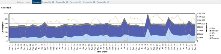
Figure 18-7. Performance data for all application calls over a two-month period, summarized by day.
The observations in Table 18-7 represent the high-level analysis of Figure 18-7. From these observations, you can determine the rate of the monthly transaction growth, see the large increase in response time, and identify potential performance issues that might occur on the weekend.
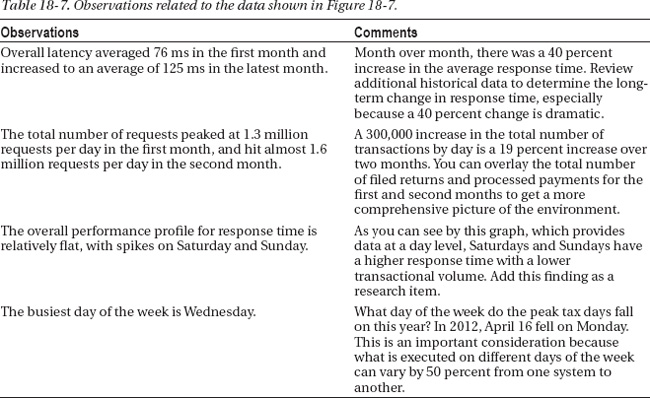
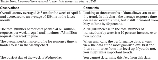
Figure 18-8 shows the cumulative number of requests and the response time by week for a three-month period. The week view provides a different view of the data, which is more helpful when you are looking for trends and anomalies.
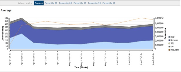
Figure 18-8. Performance data for all application calls over a three-month period, which is summarized by week.
The observations in Table 18-8 represent the high-level analysis of Figure 18-8. From these observations, you can determine the monthly transaction growth and observe a decrease, and then an increase, in response time over the three-month period.
The chart in Figure 18-9 displays the total number of requests by day and by response time. The categories can be customized to represent the SLAs, which provides another important view of the data. Following are the three categories representing the current SLA:
- Satisfied Less than 2 seconds
- Tolerating 2 seconds to 5 seconds
- Frustrated Greater than 5 seconds
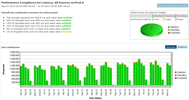
Figure 18-9. SLA compliance for all application requests by day for the last two months.
The observations in Table 18-9 represent the high-level analysis of Figure 18-9. From these observations, you can determine that the number of “tolerating” and “frustrated” requests have gone up and are higher on the weekends.
Now you have a better understanding of the usage profile for the application, but what were the utilization levels on the application and database servers? Are the database servers 25 percent or 75 percent utilized to handle 1.6 million daily requests? This is where the performance data you collected earlier becomes important.
Analyzing Perfmon Data
You might see a statement such as “The SQL Server’s CPU is averaging 25%, it is healthy and there is excess capacity.” Today’s systems and applications are very complex and cannot be measured by only a single metric like processor utilization. The % Processor Time counter is one of the many object counters you collected data from as part of this effort. Each object counter is important and tells a different part of the story. A system averaging 25 percent might be having a problem elsewhere, such as scheduler pressure, and you might overlook it by just looking at the % Processor Time data.
There are several important rules to follow when you are reviewing the performance data and working through the findings:
- When analyzing data, refer only to facts, not hypotheticals. Hypotheticals often lead people down the wrong road.
- Perform proper root-cause analysis. Many times the cause of an issue is identified without the person analyzing the data trying to understand what the real problem was. Instead, the analyst bases her opinion on circumstantial evidence that can be misleading. It would be like saying, “Johnny was in the back yard when the window was broken, so he must have done it.”
- Some object counters can be reviewed in isolation, but most object counters need to be reviewed with other related object counters. A periodic increase in I/O on the disk that contains the transaction logs is most likely the result of database checkpoints. If you review both counters together, you can correlate these events.
Analyzing performance data can be a frustrating experience for some DBAs because SQL Server performance metrics represent a small percentage of the overall object counters available and/or captured. As noted earlier, this is where the other members of the team come into play, because each one will analyze his or her respective area of the system. This enables everyone to correlate data points. A specific data point analyzed in isolation might look bad, but when you put it together with all the other information, it might be better or worse than you originally thought.
An example of this is when the Max Server Memory data for a given SQL Server instance is set to a large fixed amount that is actually starving Windows from the memory it needs. It might not be evident in SQL Server, but the OS-level counters show that there is excessive paging in the OS. When the server administrator reviews the server object counters, he might know that SQL Server is on the system but not that the internal memory setting for SQL Server is so high that it can cause such a problem. Only when the two administrator talks to another team member does he figure out that there is a mismatch. That is why communication is key within the team, especially when you are reviewing the performance data. The reality is that many non-DBAs do not understand how SQL Server works. Ensure you fully explain what you are seeing within SQL Server, and this will help others on the team make connections they otherwise wouldn’t.
If you are a DBA who likes to learn, use peak load as the perfect opportunity to learn how to analyze Perfmon data. There is a huge amount of information about Perfmon on the web that talks about the object counters and all of the recommended thresholds. There are also several great tools that can help you analyze the collected data, and templates are available that are specific to SQL Server. One of them is Performance Analysis of Logs (PAL), which you can find at http://pal.codeplex.com/. You can use this tool to analyze the Perfmon files with SQL Server–specific thresholds. After you answer some questions about the server, PAL analyzes the Perfmon file, produces a report, and outlines all of the object counters that need to be reviewed. Figure 18-10 shows sample output contained in a PAL report.
Figure 18-10. High-level view of a sample PAL report.
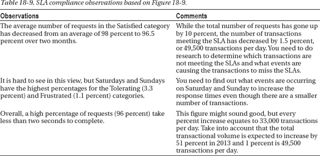
PAL breaks down a larger Perfmon data capture into smaller time slices so that numbers better reflect the performance during that specific time window. For example, if the average for PLE is calculated over 48 hours, it might include times when the buffers are under more pressure due to reindexing processes. For each time slice, the minimum, maximum, and average values for each object counter are evaluated to determine if they are within an acceptable range. If the counter is outside of this range, PAL will highlight the finding in yellow for a warning and in red for critical. The condition is shown as a hyperlink to supporting detail, as shown in Figure 18-11. Above the graph is a detailed description for the respective object counter, which is very informative, especially for DBAs who are not familiar with Perfmon data.
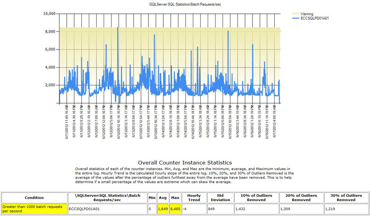
Figure 18-11. Supporting detail for Batch Requests/sec.
As you can see in Figure 18-11, additional analysis is provided if you remove the outliers for the top 30 percent and calculate the standard deviation. The data points in Figure 18-10 reflect the average over a specific time, but you cannot see the trends of the data. Reviewing the chart in Figure 18-11 provides you with a better view of the data. It is easier to see trends in the chart view than in the report view, as you will see when you analyze the Perfmon files in Performance Monitor.
PAL is a great tool for reviewing a large Perfmon file quickly, but it does not correlate the separate object counters, which as established above, is an important part of this process when analyzing the performance of complex systems. This is where utilizing the Perfmon file in binary (BLG) format comes into play. You can view the BLG file in Performance Monitor in several different formats, but the two formats I’ll walk you through are the line view and the report view. The line view displays the data in a graphical format, where it is easier to correlate the data and see trends in the data. The report view lists the values only, which makes it easier to see the values and compare them to the thresholds. You will walk through both types of formats as you analyze performance data for the example tax application.
Figure 18-12 shows the report view from a system that was run for seven days. By default, Perfmon displays the average of all values. In this view, it’s easy to see that the values for the F drive Avg. Disk sec/Read is an average of .043 over seven days.
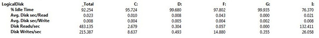
Figure 18-12. Report view in Performance Monitor for a seven-day capture of the logical disk counters.
The problem here is that the average over seven days skews the data. Realistically, you need to filter this down to, say, the core business hours. You know Wednesdays are the busiest day of the week based on data you reviewed earlier. Figure 18-13 shows how the data from the BLG can be filtered to show only data from Wednesday between 7 AM and 8 PM. To modify the Time Range setting, slide the left or right time indicator to the appropriate time.
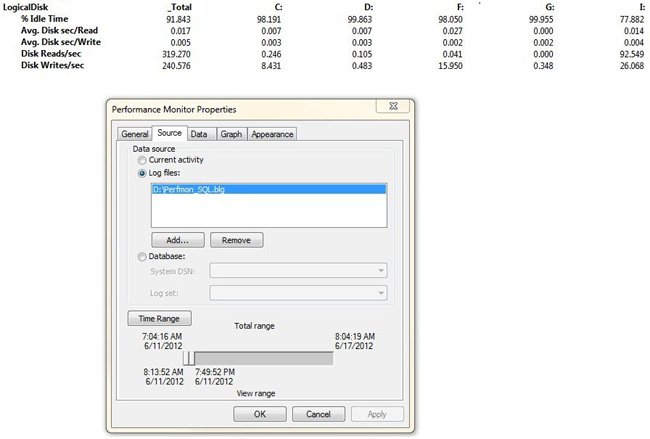
Figure 18-13. Report view in Performance Monitor for a one-day capture of the logical disk counters.
As you can see in Figure 18-13, when the F drive is viewed for the core business hours, it is .025 ms healthier than before. If you reviewed only the seven-day capture, you might believe the performance for the F drive is a lot worse than it is. You still want to understand what is causing the latency to increase to .043 ms over the seven days. To do this, you review all of the values in Figure 18-12 to determine if there are any areas of concern. Based on the numbers shown, you need to monitor the F drive’s performance over time because it is on the borderline of the threshold for acceptable performance for a transaction application.
The other view in Performance Monitor is the line view. In Figure 18-14, you can observe the Avg. Disk sec/Read performance over time. Notice the frequent spikes every 15 minutes; these are caused by transaction-log backups. One of the most important goals when analyzing the configuration or performance data is to create a mental image of the environment and be able to explain what you are seeing. Here you are looking at the disk performance, and you can see a pattern in the data. By explaining what is creating the load, you can then address the cause if necessary.
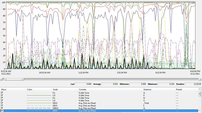
Figure 18-14. Line view in Performance Monitor for a one-day capture of the logical disk counters. The values have been scaled so that the lines are easier to read.
The other important data points in Figure 18-14 are the average, minimum, and maximum values. Because scales for the lines in the graphs are frequently different, it is often easier to review the average below the line graph. Remember, when reviewing performance data, the averages are what matter most of the time. You focus on the average of a value because that is the typical load that needs to be sustained for a period of time. If the server’s % Processor Time spikes to 80 percent once in a while, it might not indicate a problem—but it takes more information to know if that is true or not.
Reviewing the Perfmon Data File with PAL
Objective: Quickly review a large Perfmon data file, and apply the predefined SQL Server best-practice thresholds.
- Generate the report by selecting the SQL Server profile and answering all of the required questions.
- Review all warnings and critical events.
- Document any unexpected findings or critical alerts. The critical alerts might indicate potential bottlenecks, depending on the time of the day and frequency.
Review the Perfmon Data File with Performance Monitor – Report View
Objective: Review custom time windows, and see additional object counter values that are not included in PAL’s analysis.
- If the data capture is a multiday capture, filter the timeline down to the peak window.
- Review the report view first because this provides a high-level overview of the object counters.
- Add all object counters.
- The easiest way is to open the BLG file, which will add all the object counters in addition to the ones with instances.
- For items like Logical Disk and Databases, add these manually.
- Start from the top of the report, and go down while documenting all the findings.
- While you are reviewing the object counters, document your observations so that you can review them later.
- As you review the object counters, you can remove the objects that are healthy from the report view. The result is a high-level report with only the object counters you are interested in, whether they are usage based or out of compliance with best practices.
- If you want to save the images of the report, you can right-click and save the image as a GIF.
Review the Perfmon Data File with Performance Monitor – Line View
Objective: Find trends in the data over different time windows, and correlate the data from the related object counters.
- If the data capture is a multiday capture, filter the timeline down to the peak window. The non-peak window is also important to review, but concentrate on the peak window first.
- Reviewing the line view is done differently than reviewing the report view. When adding the objects to the line view, add groups of related objects together. There are a couple of important reasons for this, and the most obvious one is space. If you add 75 objects to the line view, the graph will be hard to analyze because of the large number of lines graphed. The goal of the line view is to find trends and correlate values. By adding subsets of object counters, it is easier to find trends in the data. Once the object counters are added to the graph, highlight all of the counters on the bottom and scale the lines. This increases the readability of the graph.
- For each counter on the bottom, review the line and values over time.
- Review the line over time, and identify when the counter is under pressure and for what duration.
- Review the average value. Is the counter within an acceptable range?
- How frequently is the maximum or minimum value hit and is the peak value sustained?
- Review related counters during this time to see if their values can be correlated to the event. If the value average is as expected or the counter is immaterial, delete the object counter from the line view.
- Again, remove the normal values so that the more important counters are the ones that remain.
- Once you are done reviewing a group of related object counters, you can save the image or add additional ones. Remember, the line view only has the object counters of interest. Reviewing the counters with issues along with the new counters provides you more opportunity to discover different trends in the data.
After reviewing all of the object counters, you should have a clear understanding of the peak usage times when SQL Server is under the most pressure and know what areas of SQL Server are potential bottlenecks. The other important data to incorporate into this review is the number of business transactions that were completed during the corresponding time window. With that data, you can fill in the information for statements such as the following: “My system is only 30 percent utilized when processing X number of payments.”
Analyzing Configuration Data
Typically, when a new server configuration that will run SQL Server is built, it is often done with a standard build approved by the IT organization and it’s not necessarily optimized for SQL Server. Most companies like to maintain as few server configurations as possible and make them work everywhere if possible. The build process most likely will be automated to a certain extent, with some items manually configured. The result is expected to be a server that looks, acts, and feels like all other servers within the company for a specific platform and version. Based on my experience, the standard build will usually be 98 percent correct with a 2 percent variation from the norm. The deviations are what cause problems, some of which will not be evident immediately.
Incorrect infrastructure and server configurations often contribute to performance issues. If they are caught in time, such as right after the server is handed off to the DBAs, they are easy to fix. If they are not caught in time, but are caught at some point after a server is in production, this can lead to the need to schedule downtime for the fix—even if it is easy. Some common examples of poor configurations include misconfigured memory settings, local policies, and page-file settings.
A perfect example that seemingly has nothing to do with SQL Server but, in fact, has everything to do with it are the power-management settings in Windows. A base configuration of Windows Server 2008 (or later) has a default power management plan of Balanced. The Balanced power profile turns off cores and reduces the clock speed of cores to conserve power. This throttling can impact the server’s performance. If SQL Server is installed on that server, performance could go from blazingly fast to extremely slow because of that one setting. Changing the setting is easy and might improve performance immensely. Similarly, the EFI or BIOS settings related to power might override the Windows settings, so they also need to be checked. This is another case where you need to draw all of the logical dots to come up with a single, correct conclusion.
A large part of the assessment is to collect configuration data from application servers, servers hosting instances of SQL Server, and the infrastructure. While the goal is to review the configuration of the servers and determine if they are configured correctly, what exactly is correct? Before you review the configuration data, work with the appropriate team members and get a copy of the standard build documents. The standard build should be the baseline because most companies spend a large amount of time engineering and testing the base builds. Because the standard builds might not be optimized for SQL Server, you might identify places for improvement for future builds in this process.
When you are reviewing the configurations for the various servers, keep in mind the findings from the review of the performance data. Using the example from earlier, if you see a large amount of paging in the OS and review the Max Server Memory in SQL Server, is the memory dynamic or static? Is the memory configured too high or too low? How will it need to be readjusted, or do you need more physical memory in the server? Reviewing the performance data before looking at, and possibly changing, the configuration settings provides you with valuable information you can use when you are analyzing the server’s configuration. Now you have some context for determining what the potential bottlenecks are and what areas of the system are healthy.
Because we are focusing on SQL Server, I’ll review some of the recommended configuration settings to capture, as shown in Table 18-10.
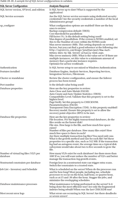
Depending on the SQL Server configuration and when the last time an assessment was performed on the server, there might be a lot of changes and tasks that result as part of the configuration assessment. For all changes, always test in a similar environment to ensure the application does not have an unexpected behavior. Production should never be the first place changes are applied. If you do not test in a similar environment first and problems are encountered, you might make things worse rather than better. Some configurations might appear to be only cosmetic, but the majority of the changes you make will change either the behavior of SQL Server or how the application will perform.
The initial Perfmon data is your performance baseline, or what the system performance was before any changes were made to the system. After changes are implemented, a new baseline will need to be created so that you can measure the percent change in the system. You can use the existing data collector to create the new baseline—just change the destination to a new file. Over time, you can start to see the impact of all the changes in the application and the system—good or bad—and adjust the configuration accordingly.
Analyzing SQL Performance Data
Tuning indexes or queries is what most people probably think about when you mention tuning a SQL Server instance for peak load. However, as you have seen in this chapter, there is a lot more to tuning for that time frame than just adding some indexes and rewriting statements. If the disk subsystem is misconfigured and you are able to perform only 10 I/O per second, all statements will suffer—even with optimized code. You might think, “How could this happen? My SAN guys told me that you had the optimal configuration.”
Here is an example from one of my past customers. This particular client was able to achieve only 10 I/Ops on its disk subsystem with reasonable performance. The server with SQL Server was configured using iSCSI to connect to the SAN. Because the disk I/O was slow, this was showing up as a performance issue to end users. It took some time, but we were able to track down the issue by working with the SAN as well as the network teams. As it turns out, the network switch that the iSCSI interfaces were plugged into was misconfigured. Because iSCSI is based on TCP/IP, the lack of performance makes sense if a key component is not configured properly. That is why it is so important to validate the underlying configuration before reviewing any part of the application. Tuning is much like peeling back the layers of an onion—you find one thing, and another gets uncovered.
So where do you start when looking at all of the SQL Server performance data if you have captured a lot of it? It can be daunting. You have data from the Dynamic Memory Views (DMV) that shows the most frequently running code, which will correlate to the largest I/O consumers. You have different data sets from Profiler or Extended Events for long-running statements or all traffic over a specific time. And what about the data set with all of the transactions that are involved in the core business transactions? As you can see, there is a lot of data—and this does not even include any of the metadata from SQL Server about object use or execution plans.
Prior to reviewing the configuration data, you reviewed the Perfmon data to provide more information about what the performance on the SQL Server instance is like. Before you review any of the information from the traces or DMVs, you need to review the current activity. The current activity of the instance that was captured earlier provides you with insight into what type of statements are executed, the common wait stats, the resource usage, and many other factors. After you do this on several of your systems, you will start to recognize patterns in the data and see when the system has an issue. Figure 18-15 is an example of the output from a script that shows details for all active process on a SQL Server instance.
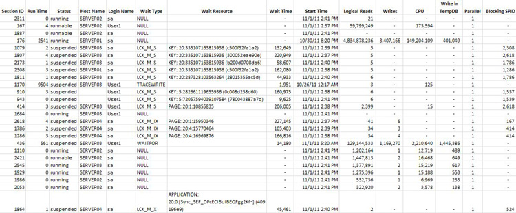
Figure 18-15. Current activity of a SQL Server instance gathered from a SQL script.
If you ran a script that generated this data several times over the course of the day, you could see patterns in the data. Following are observations from analyzing the data shown in Figure 18-15:
- There are several blocked processes, with the longest process being blocked for almost four minutes.
- Session ID is a long-running process that has consumed over 4 billion logical reads and a large number of other resources.
- Session ID 1864 is trying to acquire an application lock.
- Even though the code is not in the view shown in Figure 18-5, the sessions on the bottom of Figure 18-15 are all running the same code with a nonoptimal execution plan.
- A client-side trace is running a deadlock capture.
- There is a WAITFOR process that captures performance metrics for the custom application.
As you can see, from this one execution of the current activity data, you can identify several behaviors about this SQL Server instance. These behaviors will help you start to build the mental image in your mind about what you can expect to see as you monitor the system over time. Some of the behaviors you can expect to see are the following:
- There are large blocking chains.
- There are queries that consume a number of large resources.
- The application is using application locks in the database (
sp_getapplock).- There are nonoptimal plans for some frequently executed procedures.
There are several critical items in the preceding list that need to be addressed before the peak season. For example, at the beginning of the chapter we talked about large blocking chains that are impacting the application. The blocking chain in Figure 18-15 was impacting users for a minimum of 4 minutes, and this potentially could cost the business thousands of dollars in potential orders.
Additional information needs to be captured for all of these items. You need to identify the unique blocking chains, when they occur, and what objects and processes are involved. Another source of blocking information is the sys.dm_db_index_operational_stats DMV, which you can use to see which objects are frequently waiting on locks or have lock contention. Frequently executed statements need to be tuned and potentially rewritten to minimize the chance of receiving a nonoptimal execution plan. The goal for the core business transactions is for them to be predictable so that they can meet the performance requirements in the SLAs. If several stored procedures involved in a core business transactions have a large runtime variance, the risk of not meeting the requirements of the SLAs increases. The next step addresses the large resource consumers because we’ll review the runtime data that we captured from SQL Server and the application.
Begin by reviewing the index utilization statistics that were captured during the data-collecting stage. Index changes are usually low-risk and high-reward changes to make. If you adjust the indexing strategy on the core tables, you can have a positive effect on a large number of SQL statements. If you start by tuning SQL statements, the risk is higher. Tuning SQL statements requires more effort and a significant amount of testing. After you adjust the indexing strategy and affect many of the execution plans, you will be in a better position to review the runtime performance for the SQL statements.
Figure 18-16 represents a sample data set you will review. It is a subset of the result set for index usage data. Additional columns included in the view are server name, database name, source, object name, object_id, index name, last user scan, last user seek, and run time.
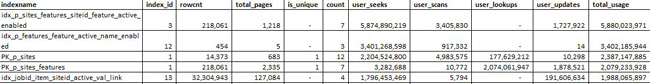
Figure 18-16. Usage statistics for all indexes.
Figure 18-16 shows index usage statistics and some other metadata about the indexes on particular objects. This data includes many attributes that are essential for the analysis, such as is_unique, rowcnt, total pages, and the total number of indexes on a table. From this data, you can determine the following scenarios:
- Unused indexes Indexes that have not been used.
- Costly indexes Indexes that require more resources to maintain than is warranted by how much the index is used.
- High number of indexes Review all tables with a large number of indexes. What is considered to be a large number of indexes? The answer to this depends on which of the following types of applications SQL Server is supporting:
- Transactional Database For this type of database a large number would be about three to five indexes per table, but what qualifies as “a large number” really depends on the amount of system activity.
- Reporting Database For this type of database, a higher number is acceptable, but a large number might affect the extraction, transformation, and load (ETL) performance.
- Mix – Transactional and Reporting Database If both of the preceding types of databases are used, about five to seven indexes per table is considered to be a large number. However, it really depends on the amount of system activity.
- Missing indexes Larger objects with high scan counts are candidates for additional indexes.
- High number of lookups Review the most frequent statements against the object to see if adding a couple of columns might help offset the need for a lookup. Remember, leverage INCLUDE columns but consider the index width.
- Non-Optimal Clustered Key Notice the nonclustered index in Figure 18-17 with a lower number of seeks and a high number of lookups on the clustered index. This indicates the common access path into this table is on PK_Table1 than on CDX_Table1. Consider changing the columns that are clustered in this example.

Figure 18-17. Usage statistics for a table that needs the clustered key switched to another column(s).
![]() Note After the new index changes have been implemented, you need to collect updated DMV performance data as shown in Figure 18-16 and trace data, as shown in Table 18-5 because the index statistics and performance profiles will have changed.
Note After the new index changes have been implemented, you need to collect updated DMV performance data as shown in Figure 18-16 and trace data, as shown in Table 18-5 because the index statistics and performance profiles will have changed.
After you have performance-tuned a system several times or even tuned the same system over time, you will start to notice that tuning indexes gets you most of the way to where you need to be. Adjusting configurations, the timing of events, and code will get you the rest of the way.
There are several approaches you can use when identifying which SQL statements to performance tune. Following are different sources, in order of preference:
- Top 100 Query Stats by Execution Count These frequently called statements represent the majority of the total resource consumption. If 75 percent of these statements are tuned with indexes or code modifications, you will reduce total resource consumption by a large percentage. Remember, people and time are usually limited, so spend your time tuning processes that will have a large impact on the system. Do not tune the one query that uses 500 million I/O because this is not an effective use of time and the net savings you’ll see in terms of system resources is not as great.
- ALL statements from the core business transaction Evaluate these because they have a direct impact on the user experience. If you make these statements faster, the user experience will most likely be better.
- SQL statements that frequently receive nonoptimal plans and are frequently called Based on my experiences, nonoptimal plans are usually magnitudes worse and could cause additional issues on the server.
By adjusting the indexing strategy and performance tuning of the most frequently called procedures, you can reduce the total resource consumption of the server. There is often a single large query that consumes a lot of resources, but tuning that should be secondary to one that is executed 1,000,000 times per day. Once the changes are implemented, measure the new resource levels as talked about earlier to see if things are better or worse. This is an iterative process, so make sure to collect updated metadata and runtime statistics.
At the end of this exercise, if you determine that the current environment will not be able to handle the peak load, start to think about other environmental or process-related changes. Not every change needs to be a code or configuration change. If reporting is going against the transactional environment and the total resource consumption is 25 percent, can you shift this to another server running SQL Server? If you only need 5 percent to 10 percent more resources, what can be delayed or turned off during the peak load? Can you run the maintenance processes two days before? What about disabling nonessential processes? When you are tuning for peak usage, every option should be on the table. Sometimes you need to think outside of the box because certain environments have some unique challenges.
Devise a Plan
So how do you translate all the analysis and findings into an actionable plan? As you have done up until now, you need to take your time and review all of the findings to come up with the right solutions. The challenge now is determining what change you implement first, and what the expected impact and potential risks are of applying that change. Are there any system limitations that you identified earlier that might impact the potential changes—including figuring out whether the change can even be implemented? These questions are complex and the potential impact of your decision is often not fully understood until the change is fully deployed into a test or production environment.
The same way that you started to analyze the data, you will implement the proposed changes. Always start with the configuration changes. These will correct misconfigurations in the environment or change the behavior of the respective technology. For example, if you choose Optimize For Ad-Hoc Workloads option in SQL Server, this will change the behavior of SQL Server and reduce the amount of memory consumed by the procedure cache at the instance level. After you make a change, make sure you document the actual result of the change if possible. This way, you can have a record of the action and result just in case there is an issue later on and the change needs to be rolled back.
Table 18-11 is the sample order of proposed changes for the tax application. In addition to the server-specific changes shown in Table 18-11, there can also be application, infrastructure, and process-related changes.
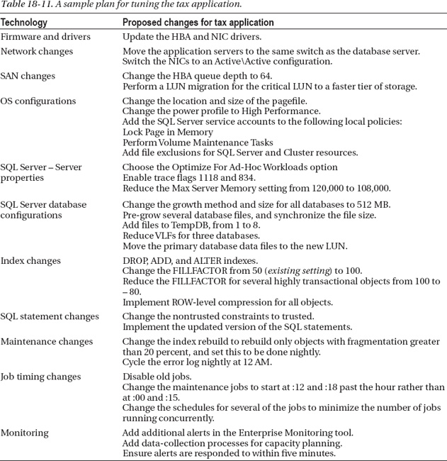
Something that cannot be overemphasized is ensuring there is sufficient support from the developers and all levels of operations during the peak load. If issues occur during this time, people need to be able to respond in a timely manner. Depending on the SLAs, the response time might be minutes rather than an hour. Processes and procedures need to be defined and clearly communicated to the staff.
Conclusion
Every DBA has servers running SQL Server that must perform and scale day after day, year after year. Over time, things change. The data grows, the load and usage patterns might increase, and the functionality often evolves. So what will you do this peak season to ensure your organization is able to process this year’s peak load? What lessons did you learn from last year’s peak load so that you don’t have the same problems?
By creating an ongoing team that is capable of analyzing the environment and implementing necessary changes, you will have a head start toward making sure the environment can scale to meet increased demands, whether it is the Black Friday sales day or just a busy Wednesday. Things will change in the environment and with the application, but these changes might bring more opportunity, such as long-term recommendations being folded into the application design or the architecture of the entire solution being changed. The key to being successful is to be curious and look under all of the rocks and behind all of the doors for opportunities for improvement.