CHAPTER  13

I/O: The Untold Story

By Jeremy Lowell

We are living in an age when data growth is being measured in factors over the previous decade. There’s no indication that the rate of growth will subside. This pace is here to stay, and it presents companies and data professionals with new challenges.

According to Gartner (http://www.gartner.com/it/page.jsp?id=1460213), data growth is the largest challenge faced by large enterprises. Not surprisingly, system performance and scalability follow close behind.

In an unscientific study based on conversations I’ve had with many database administrators (DBAs) and other personnel in companies I have the honor of working with, I’ve found that they are struggling to keep up with this data explosion. It’s no wonder that DBAs share one of the lowest unemployment numbers in the technical field. The purpose of this chapter is to provide DBAs with the knowledge and tools to drive this conversation with your company, your peers, and that wicked smart storage guru in the corner office.

How many times have you entered a search in Google related to I/O and come up with either a trivial answer or one so complex that it’s hard to fully understand? The goal of this chapter is to help bridge that gap and fill in the blanks in your knowledge regarding your database environment and the correlating I/O.

I/O is often misunderstood with respect to its impact within database environments. I believe this is often due to miscommunication and a lack of foundational understanding of how to measure I/O; what to measure; how to change, modify, or otherwise alter the behavior; and perhaps more importantly, how to communicate and have the conversation about I/O with peers, management, and of course the storage and server gurus whom we all rely on. As you delve into this chapter and learn how to better measure, monitor, communicate, and change your I/O patterns, footprint, and behavior, it’s important to begin from a common definition of “I/O.”

A distilled version of I/O, as it relates to this chapter, is “Data movement that persists in either memory or on disk.” There are any number of additional types of I/O, all of which are important but fall outside of the context and focus of this chapter.

The untold story of I/O is one you have likely struggled with before—either knowingly or unknowingly—and it contains within it a number of very important data points for your database health, consistency, performance, and availability. This chapter will focus on two primary types of I/O: memory (logical I/O) and disk (physical I/O). Although they are intimately related, they follow different patterns, and different approaches are required for measuring, monitoring, and resolving issues with each of them.

The Basics

The beginning of this quest starts with preparation. In this case, with understanding what your database system requires of your disk subsystem during normal operations, peak loads, backups, subsystem (SAN) maintenance, and what appear to be idle periods.

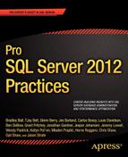
Baselining your database, server or servers, and environment is critical to understanding the I/O characteristics of your system. More importantly, it helps you to determine if there’s an issue and where its origin might lie. There are a handful of metrics you need to obtain and whose trends you need to monitor over time. Table 13-1 shows sample output from the counters you can use for this, and they will be explained in further detail as you dive deeper into the chapter.

The source for the data in Table 13-1 is Performance Monitor. Performance Monitor is a utility found in Microsoft operating systems which graphs performance related data. In the “Tactical” section of this chapter, you can find details on how to configure counters in Performance Monitor.

There are two primary counters found in Performance Monitor for the counters referenced in Table 13-1: the Logical Disk counter and the Physical Disk counter. I prefer the counter Logical Disk for a number of reasons, but an understanding of the primary difference between the two can be found in the description of the counters, which in part reads, “The value of physical disk counters are sums of the values of the logical disks into which they are divided.” As such, the Logical Disk counter provides you with a lower level of granularity, and I’d argue it gives a more accurate depiction of how the server—and thus, the database—is performing on that drive. It’s also a more intuitive way to look at the disks on the server because most DBAs know which database files live on which drives.

Monitoring

The counters I prefer to base decisions on have changed over time. Years ago, I relied on the Disk Queue Length counter. This counter measures the queued requests for each drive. There is a common rule which states that a sustained value above 2 could be problematic. The challenge with this value is that it must be a derived value. To derive the correct number, the quantity of disks or spindles involved must be taken into account as well. If I have a server with 4 disks and a queue length of 6, that queue length appears to be three times higher than the threshold value of 2. However, if I take that value of 6 and divide it by the quantity of disks (4), my actual value comes out to 1.5, which is below the threshold value of 2. Over the years, storage vendors have done some wonderful work, but it has left others wondering how to adapt to the changes. This is the reason that I leave out the counter I relied on many years ago and now my primary counters deal with how much data the database is moving to the storage subsystem (Disk Bytes/sec), what type of bytes (read or write) they are, how many of them there are (Disk Reads/sec) and (Disk writes/sec), the size of the I/O request (in and out requests per second) (Avg. Disk Bytes/Read) and (Avg. Disk Bytes/Write), and finally how quickly the storage subsystem is able to return that data (Avg. Disk sec/Read) and (Avg. Disk sec/Write).

This set of counters yields interesting data, all of which happen to be in a language your server administrator or your storage guru can relate to. Note that when your operating system (OS) reports a number, it might not be the same number that the storage device is reporting. However, it shouldn’t be far off. If it is, it’s often due to the sample interval that each of you are independently working from. Traditionally, storage area network (SAN) metrics and reporting aren’t sampled at a frequency of one second. However, servers are often sampled at this frequency, and for good reason. The sample set is typically sourced from Performance Monitor, and it’s only captured during times of interest at that poll frequency. The result is that when the conversation begins, you need to ensure that everyone is talking about the same apples—this includes the same server, logical unit number (LUN), frequency of the sample (sample interval), and of course time frame. Time frame is certainly important here, because averages have a way of looking better over time.

There’s an interesting relationship between all of these counters which helps to explain the I/O behavior on a database server. As you can imagine, if the Disk Reads/sec (read In/Out Per second, IOPs) increased, one would expect the Disk Read Bytes/sec counter to increase. Typically, this is true, but what if, at the same time, a different profile of data were accessing the database server and the Disk Bytes/Read decreased? In this manner, you certainly could have more I/O requests per second, at a smaller size, resulting in the same Disk Bytes/second measure. It’s for this reason that knowing and understanding your specific I/O footprint and pattern is so important. There are times of the day that your system will behave in a certain fashion and other times of the day when it’s significantly different.

Considerations

Imagine that your database server supports an online retail store where 99 percent of the orders and the web traffic occur between 8:00 AM and 5:00 PM. During that time of the day, your I/O pattern will be indicative of what the web application needs in order to fulfill orders, look up item information, and so forth. Of course, this assumes you don’t run database maintenance, backups, Database Console Command’s (DBCCs), and so forth during the day. The only thing running on the database server during those hours are applications that support the online web application r applications. Once you have an understanding of what that I/O profile looks like, it will give you a solid foundation to begin from.

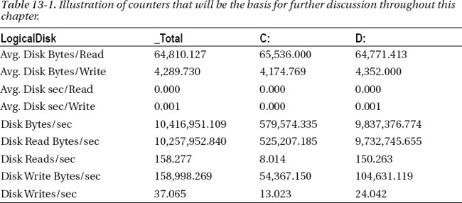
At this point, if you are anything like me, you are thinking to yourself, “Can’t you just show me a picture, already?” Indeed, often it can be easier to visualize the relationship between counters to see why they matter. Figure 13-1 shows that relationship.

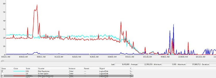
Figure 13-1. Illustration of Disk Reads/sec (Bold), Disk Read Bytes/sec (Normal), Avg. Disk sec/Read (Light), and Avg. Disk Bytes/Read (Dash)

This is an interesting view of the logical disk because it shows that the relationship of IOP size (Avg. Disk Bytes/read), disk throughput (Disk Read Bytes/sec), and the quantity of IOPs (Disk Reads/sec). The Disk Reads/sec counter (the bold line) shows a very steady size for the majority of the sample, but as you can see early on, there was an increase in the size of the I/O, which translated into nearly a threefold increase in disk throughput.

This means, in short, that not all I/Os are created equal. As you can see in Figure 13-1, a variation in the size of the IOP can have a noticeable effect on the environment. One of the primary reasons I look for this and make note of it is so that I’m not surprised when this occurs in an environment. Imagine that you are working diligently on providing scalability numbers for your environment and one of the key performance indicators (KPIs) is “business transactions.” In this context, the application group makes a statement along the lines of “You do 1,000 transactions per hour during the day and 100 transactions per hour at night,” and you are asked what that means at a database level. In this scenario, the business also wants to know what it would mean if the transaction rate remained the same yet native growth of the database continued over the period of a year. They also want to ensure that the next hardware purchase (the server and SAN, specifically) will provide enough horsepower to further the native growth of the database and also a potential transaction increase from 1,000 per hour to 2,000 per hour.

At first blush, this scenario seems simple: double what you have and you will be OK. But what if that simple math didn’t actually pan out? What if, due to “wall-clock” time and service times on the SAN, there suddenly weren’t enough hours in the day to update your statistics, rebuild your indexes, execute DBCCs, or keep up with the backup window?

Typically, there’s not a linear increase with data growth over time. For many businesses, the customer base is expanding, not contracting. These additional customers will slowly add to the size of your database and require additional I/O that you cannot see a need for in your data today. Even in the scenarios where the customer base is contracting, it’s common that data is kept for the old customers. This happens for a variety of reasons, including regulatory, marketing, financial, and so on. The result is that, while it’s tempting to rely on the simple math, doings so can result in some complications down the road.

For this reason, understanding your I/O profile over time and knowing which data is in the mix is critical.

The type of I/O will change based on the type of business transaction or the operation you have written or scheduled. Backups, for instance, have a very different I/O profile than traditional business transactions, and even business transactions are not created equal. Consider a company that sells widgets online and via an outbound call center. The type of I/O for the online web store might have differing characteristics than the client-server application that’s used by the outbound call center employees.

Another interesting example is determining what type of reporting occurs against your OLTP database server and even the times that the reports are run. Often, operational types of reporting occur during the day, while summarized information or rolled-up data reporting occurs during the evening hours. But what if users have the ability to run the larger, more I/O-intensive rollup types of reports at, say, the end of each month in the middle of the day? What if that coincides with a marketing push and your web store traffic increases by 50 percent?

What if your environment is configured in such a manner that you have a multinode cluster in which all clusters reside on the same SAN? In that scenario, when you are doing your nightly maintenance (backups, index maintenance, DBCCs, updating statistics, user processes, and so forth), the job to populate your data warehouse is also pulling large amounts of data from your OLTP database into your staging environment, and then munging that data into your star schema. You can see that during that time, no single server will appear overloaded; however, they all share the same storage array and, likely, the same controllers and, many times, the same spindles (disks). Suddenly, your scheduling takes on new meaning. Ensure that your scheduling is thought through from an environment perspective, not just at a server level. Every shared component needs to be taken into account.

Tactical

As you go through the process of measuring, monitoring, and trending your IOP profile, bear in mind the ever-important Avg. Disk sec/Read and Avg. Disk sec/Write counters because they are critical to your I/O performance. They measure the duration it takes to read and write that specific IOP request to the disk. In Table 13-1, you can see that the disk I ran a test on is very fast, taking 0.000 seconds (on average) to read from the disk and only .001 seconds to write to the disk.

In my experience, it’s difficult to find an authoritative source for what these numbers should be. This is due to the quantity of variables involved with reading from and writing to disk. There are different speeds of disks, sizes, manufacturers, seek times, scan times, throughput metrics, SAN cards, SAN card configurations, SAN configurations, OS configuration, LUN layout, and database settings. Most importantly, there are also differences in your database, its access patterns, data types, and size, to name a few. I believe it’s due to those variables that vendors, SAN manufactures, server manufacturers, Microsoft, and even experts in the field hesitate to provide hard-and-fast answers. With all of that said, the numbers in Table 13-2, in part, are subject to the variables I just listed, as well as any number of additional items that I have yet to come across.

Table 13-2 represents a best-case scenario for how long it should take your subsystem (disk) to return data to the OS based on the counters Avg. Disk sec/Read and Avg. Disk sec/Write.

The numbers in Table 13-2 are given in fractions of one second, and it’s often easier to have this illustrated and communicated in milliseconds. By multiplying the values shown in the table by 1,000, the time will be displayed in milliseconds (ms). Throughout this chapter, when disk read and write time is referenced, it will be shown in milliseconds.

Armed with this as a guideline, be aware that there are additional variables to take into account that can and should be taken into account when you’re striving to better understand your I/O footprint or resolve a potential issue in your environment. The specific variables are TempDB and transaction logs. You also should keep your application in mind. If you support an ultra-low latent application—such as those found in the credit card industry or trading industry, such as the stock market or energy market—these numbers are likely not applicable. Alternatively, if your application supports a mail order catalog, which has no user front end and is predominately batch in nature, these numbers could be too aggressive. Again, it’s all relative. The intent of providing the numbers in Table 13-2 is to give you a gauge of what I’ve commonly seen over the years with a variety of applications and I/O requirements.

Logs are more impacted by long write times and, depending on the environment, can become problematic by having long read times as well. Each transaction in a database that requires an element of data modification (Insert, Update, or Delete) is a logged operation. This is always the case, regardless of the recovery model in place. As such, ensuring that the write time for your transaction logs is as low as possible is perhaps one of the most important things you can do within your database environment.

A practical way to think about this is in terms of write transactions per second. This counter is interesting to look at in combination with transactions per second because it illustrates how many transactions are dependent on the write time to the transaction log. If you couple this value with the Avg. Disk sec/Write, you can often find a correlation. The reason that this matters is that if your database environment is adding 20 unnecessary milliseconds to each write transaction, you can multiply the quantity of write transactions by the quantity of milliseconds to further understand how much “wall clock” time is being spent on waiting for the storage array to tell the OS it has completed its operation. As you do that math, watch your blocking chains and scenarios and you will likely see that you have a higher number of blocks during the longer-duration log write events.

The size of the I/O request also plays a part. The size refers to how much data exists for each request. Traditionally, read IOPs will have larger blocks than write IOPs. This is due, in part, to range scans and applications selecting more data than they write. This is another area where understanding your I/O profile is very important. For instance, in the evenings when re-indexing occurs, you’ll likely see higher values for the size of your IOP request than you will see during the day. This is because the sizes of the transactions you are working with are much larger than individual inserts or updates, which are traditionally very small. Imagine the scenario where you have a solid understanding of your I/O pattern yet you notice that your Disk Bytes/sec counter varies. The problem here is likely the size of the I/O request. It’s important to understand that these counters work in concert with one another and, in their completeness, the full picture can be seen and your true I/O pattern can be realized.

At this point, you should have a good understanding of how to monitor your I/O. Over the course of this chapter, a harder portion of the equation will be factored in as well. The aforementioned equation includes some of the variables mentioned previously, specifics unique to your environment and database, and, of course, some suggestions for what can be done about decreasing or changing your I/O footprint and/or pattern.

To monitor your I/O, open Performance Monitor, expand Data Collector Sets, right-click User Defined, and select New. That will bring up the screen you see in Figure 13-2.

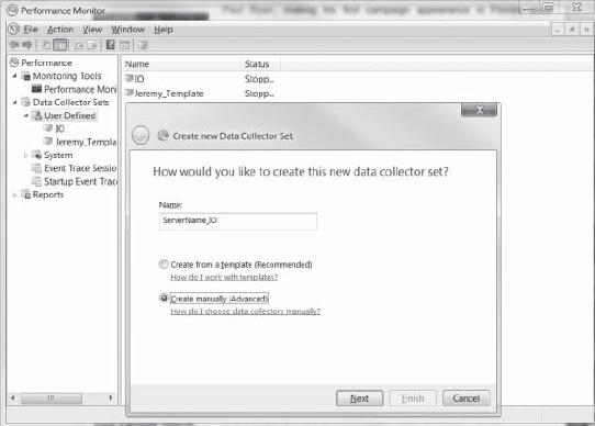
Figure 13-2. Creating a new data collector set using Performance Monitor.

Choose Create Manually, click Next, and then choose Create Data Logs and select Performance Counter, as shown in Figure 13-3.

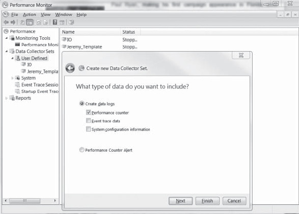
Figure 13-3. Specifying the type of data to collect with Performance Monitor.

Click Next, set the sample interval to one second, and then click Add. Then choose Logical Disk and, for the sake of simplicity, choose All Counters and <All Instances>, as shown in Figure 13-4.

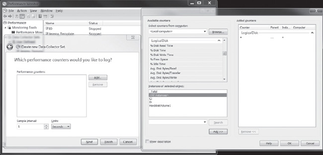
Figure 13-4. Specifying which counters to use in Performance Monitor.

You will then choose where you want the file written to. As you become more familiar with Performance Monitor, you will find that Log Format, Log Mode, and additional options that can be helpful depending on your needs.

Now that you have numbers in hand… (Oh, didn’t I mention earlier that there would be some required work associated with this chapter?) If you don’t yet have your IOP numbers, go get them—I’ll hang out and watch another episode of Mickey Mouse Clubhouse with my daughter.

Later, you can work on refining your process, your data-collection times, your reporting for this data, and so on; for now, know what your numbers are. Without knowing your I/O profile inside and out, how can you ever know if it’s good, bad, or an issue at 3:30 AM on a Saturday morning after a fun night out on the town? Trying to figure this out while in the midst of a performance meltdown of your .com server on Super Bowl Sunday is not only a way to develop ulcers, it could be the demise of your tenure at FillInTheBlank.com.

Code or Disk?

I’ve read many articles and books over the years that state, in part, that not having backups is an inexcusable offense for a DBA. I couldn’t agree more with that sentiment, but honestly, that bar is pretty low and I think we’re all up for raising it a few notches. So let’s throw I/O into that mix as well.

One of the questions I often receive is along the lines of “Is this bad code or bad IO?” I love that question because the answer is typically “yes.” Of course your system has bad code. Of course your environment has bad I/O. There’s no such thing as “good I/O” in a database system, where I/O is the slowest portion of the database environment. Well, it should be. If it isn’t, read other chapters in this book!

So what’s to be done about this? Let’s begin with the I/O pattern, which was covered earlier. In most database environments, the I/O pattern will look very familiar day to day and week to week. Often, this I/O pattern looks the same during different times of the month as well, (Think about a retail store that is open from 8 AM to 5 PM and records inventory or reconciles its balances once per month or a traditional financial institution that sends out monthly statements at the end of each fiscal month.) The examples could go on forever, and you have an example of your own that you should be aware of, based on the business your database supports.

The I/O pattern is a valuable and actionable data set. With it, scheduling can encompass much more than just your database server because most environments contain shared storage (SANs or NASs) and these shared-storage appliances have their own maintenance windows, their own peak windows, and so forth.

Once we are all working from the same sheet of music, it’s much easier and more effective to communicate challenges. These challenges aren’t experienced by you alone. This is very important to understand. If you are on a shared storage device, other application owners are encountering the same challenges that you are. The difference here is that you can be the one to drive the conversation for everyone because you are armed with data and you know your schedule and when you need certain IOP throughput from your shared storage device. I cannot emphasize enough the importance that this conversation will have within the various groups in your organization. This will build bridges, trust, and confidence. It will enable the SAN gurus to better understand your needs and why they matter, and it will enable the server administrators to change their system backup windows or virus scans to a different time. In short, it enables communication and collaboration because having such discussions without data, without the facts, it can come across as finger pointing or an attempt to shift the blame.

One of my favorite conversations with clients revolves around this topic because it’s easy to take ownership of your database being “hungry” for IOPS. If the value and necessity of it can be clearly communicated with hard-and-fast data points, well, how can you go wrong? How can your organization go wrong?

Moving on, the point of the previous section was to introduce you to the metrics and to explain why they matter, what can be done with them, and how to obtain them. Now that you have them, let’s talk about a few of the finer points.

In your I/O profile, you will likely see that during different times of the day your I/O pattern changes. Take, for example, the Disk Bytes/sec counter. If you see significant and sustained changes in this counter, check the related counter, Disk Bytes/Read(Write). You’ll likely see a change in the size of the I/O because different types of IOPS are used for varying database loads. While looking at this, go ahead and look at the Disk Reads(Writes)—the correlation should be pretty clear. You will see that during your backup window, the quantity of IOP is decreased while the throughput is increased, and the size is likely elevated as well. The same will be true for re-indexing activities.

Consider changing your backups, re-indexing, or statistic updates to times when your subsystem can better handle that type of load. When you contemplate changing this, you should communicate it with your system administrator and SAN guru, because they will appreciate the communication and might change something on their side to accommodate your need.

Now on to more specifics because, as they say, the devil is in the details and there’s nothing like having your environment, including your I/O pattern pretty well understood and then being surprised. One of the key elements with this monitoring and analysis is to do it by LUN. Ideally, your database files are broken out on different LUNs. For example, having the log file on a separate drive makes monitoring easier, so is having TempDB broken out to a different drive. This is because the I/O pattern and type vary with these specific workloads, unlike the user databases in your environment. The log files, for example, will require the lowest possible write latency because every transaction is dependent on this file. If you have replication enabled, note that there will be some reads as well, but the more important aspect with your transaction log is that the writes need to be as fast as they can be. TempDB is a different beast, and it’s used for a number of different functions within the RDBMS, such as for table variables, temp tables, global temp tables, sorts, snapshot isolation, and cursors. Because of the dynamic usage of TempDB and the elements which are enabled in your environment, you need to not only tune TempDB from a file management perspective, but also from an I/O perspective. This takes two forms: decreasing latch contention, and increasing throughput in TempDB. After all, the intent of having multiple data files for TempDB is to increase throughput in TempDB, which translates to increased throughput to the disk. If the disk cannot adequately support that throughput, the intended gain cannot be realized. TempDB usage, due to the quantity of operations that can occur in this database, can be more challenging to identify a known I/O pattern. Keep in mind that if you find slow I/O in TempDB, the scenario is similar to a slow log write except that your primary impact are to reads.

Times Have Changed

Many years ago, the predominate method of attaching storage to a server was to procure a server with enough bays, find a controller that could support your redundant array of independent disk or disks (RAID) considerations and throughput requirements, and then find the drives that were the correct speed and size for what you needed.

As a simple example, suppose you have three hard drives. Believe it or not, this was a common configuration years ago, and often these three drives would be provisioned as a RAID-5 array, often with two logical drives partitioned.

Understanding the types of RAID will help you develop a solution that’s in the process of being designed or configure an existing solution that is either being refactored or scaled up. In today’s world, the ticky-tack details of RAID inside of current SANs is a bit different than it used to be, but you need to understand some of the underpinnings of the technology to better appreciate what the storage gurus do in your company. Developing such an understanding might build a communication bridge when they learn that you know a thing or two about their world.

You can think of RAID, in its simplest form, as taking the three disk drives, pushing the magic “go” button, and transforming them into one viewable disk from the operating system and by extension, SQL Server. Now that you have a drive with three disks, you can have bigger LUNs and more easily manage the OS and the databases that reside on the server. At this point, you are probably thinking the same thing I thought when I wrote that, which is “That’s what those storage gurus get paid for?” Clearly, there’s a bit more to it than pushing the magic “go” button. Just imagine if the storage gurus always gave you what you asked for. In this case, you would have one “drive” with your logs, data, OS, TempDB, and any third-party software you use on your server. Suddenly, the file structure on your server looks like the one on your laptop, and most folks aren’t happy with the performance of their laptop when they are saving a big file or unzipping a .blg they just copied from their server to get to know their I/O pattern.

The primary purpose for the drives on your servers implementing a type of RAID is fault tolerance. In today’s world, anyone can walk into a big-box electronics store and buy a terabyte of hard-drive space for less than $100. Compared to commercial-grade drives, that is a very good bargain—but somewhere you hear your grandfather’s wisdom whispering, “You get what you pay for.” While the quantity of storage per dollar reaches historically low levels year after year, the performance and availability of those hard drives hasn’t had a similar increase. This means that if one terabyte of storage cost $1000 US dollars just five years ago and now it’s $100 US dollars—a tenfold decrease—the availability, durability, and speed of that terabyte of data has not increased tenfold.

You also need to have a good grasp on the types of RAID. RAID 5 was the primary RAID configuration that I learned about, and it’s still one of the most frequently used type in the industry. The concept of RAID 5 is akin to striping a file across all of the drives involved and then adding parity. In this manner, any singular drive in a three-drive configuration can fail and the data will still be available until such time as the drive is replaced and the data is then written to the new drive. This is perfect when the intent is to have fault tolerance with a hard drive. However, it comes at a price. In this case, that price is performance. For RAID 5 to be successful, it must read the data you are accessing, and if you modify it, it must re-read the block to recalculate the parity, write the data, and then rewrite the data to maintain parity. This becomes a performance bottleneck rather quickly, and it’s why you will see many blogs recommend that SQL Server transaction logs and TempDB be located on RAID 1+0 (10).

RAID 10 is arguably a better form of RAID for database systems because this form of RAID obtains its fault tolerance from mirrors of information and its performance from striping the data across all of the spindles (disks). Due to the definition of the word “mirror,” the three-disk configuration I mentioned earlier wouldn’t work for RAID 10, but if you had a fourth disk, you could implement RAID 10. This mean that the write penalty wouldn’t be as significant as with RAID 5 but the usable space is now only roughly half as much as the storage you purchased, because the data is being mirrored. In our configuration with RAID 10, two of the drives simply mirror the other two, which means that our footprint for available data is half of the storage purchased. From a performance perspective, this is a much better way to go because the mirrors can be read from, and to support your data footprint, more spindles need to exist.

There are additional types of RAID. I could attempt to explain them all in this chapter, but your eyes are likely rolling back right in their sockets at this point and you are probably wondering, “Why do I care?”

You need to care because if your storage guru asks what you want, you can confidently say “I’d like a double pounder with cheese and a….”. Back up—you aren’t that cozy with your storage guru, yet. Arming yourself with knowledge about RAID and your specific SAN is invaluable when it’s time for your storage guru to assign you LUNs for your database. It provides you with the opportunity to have an educated conversation with him and request what your database longs for: fast I/O. It was mentioned earlier that Transaction Log files and TempDB are both susceptible to slow I/O, and I/O waits are the bane of a well-performing database system.

In the majority of environments today, SQL Server database storage is often found on shared disk (SAN or NAS). Many of these appliances will have hundreds of spindles. If you consider the example we’ve been discussing with three disks, you can see how much this changes the landscape for your environment. One would immediately think “Yahoo! I have more spindles.” Yes, you do—but with that, you typically have other applications on those same spindles.

For instance, what if the storage appliance your database is on also houses your Microsoft Exchange environment, SharePoint, middle-tier servers, web servers, and file shares? Suddenly, you find yourself competing for I/O with the shared-storage appliance and controller or controllers on that appliance. This not only changes the landscape, it also introduces some complexity in monitoring and measuring the performance of your database. This means you need to dive a bit deeper than just Performance Monitor numbers. If you have data points in hand and knowledge about your storage guru’s world, you can better communicate what your database needs in order to support your SLA or the businesses expectations with regard to performance.

Getting to the Data

With the Performance Monitor data you have in hand, you can see the impact that slow disk-access time has on your database by querying the Dynamic Management Views (DMV) in SQL Server. SQL Server offers a number of DMVs that can be used to dig deeper into the causes of your I/O, in conjunction with external data such as that provided by Performance Monitor.

The data set from the DMVs, in the query referenced next, can be queried, and it will return what’s known as disk stalls. This result set is significant because it begins to narrow down which of your data files (databases) is driving your I/O.

In traditional Online Transactional Processing (OLTP) databases, the majority of I/O is consumed via reads. The percentage of reads compared to writes in most OLTP workloads follows the 90/10 rule. This is to say that 90 percent of the data your database server will present is for read operations and only 10 percent will be written. This number, however, is significantly skewed (in a good way) due to RAM. The more RAM you have, the more data you have in cache and, as such, the less data you have that needs to be retrieved from disk. The ratio of how much data is read from disk or written from disk varies significantly based on the usage patterns, access paths, indexing, available memory, workload, and so forth. As a result, it’s important for you to know what your database server’s ratio is. Again, keep in mind that backup operations, DBCC CheckDB, reindexing tasks, updating of statistics, and any number of additional database maintenance tasks can significantly alter the result set because this data is cumulative since SQL Server was last restarted.

Without further ado, the following query will begin to answer these questions for you:

Sample output for this query can be found in Table 13-3.

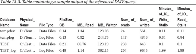
This is an interesting data set because it helps to illustrate which specific database is driving your IOPS higher.

The result set columns that aren’t apparent are as follows:

• FileSize_GB This is the size of the file as persisted in the dm_io_virtual_file_stats DMF.
• MB_Read The quantity of MB read from this data file.
• MB_Written The quantity of MB written to this data file.
• Number of Reads The quantity of reads from this data file.
• Number of Writes The quantity of writes to this data file.
• Minutes of IO Write Stalls The aggregated total of all of the waits to write to this file.
• Minutes of IO Read Stalls The aggregated total of all of the reads to this data file.

The values in this table are certainly useful, yet they contain information since the instance was last restarted. Due to this, the values reported are going to contain your backup I/O, your re-indexing I/O, and, of course, normal usage. This tends to skew these numbers and makes it challenging to know when the reported waits are occurring. One option is to create a job that persists this data at an interval. In this manner, it is easier to tell which databases are consuming the majority of I/O and, more importantly, identify the related stalls. I/O stalls are not a bad thing, and they will occur. However, if you see a significant deviation between your files and find that your log files have a high number of stalls associated with them, you need to determine if they are related to checkpoints or normal operations. A good way to tie this information together is via the wait statistics, per server, which are available via the sys.dm_os_wait_stats DMV. This DMV is also cumulative and provides some excellent information about your overall wait types. Armed with data in this DMV, you can begin to figure out what’s causing the I/O stalls.

Even with that subset of information, it might not be clear what you need to address. That’s where the session-level information begins to be of value.

The following query will begin to provide the actual T-SQL that is driving your I/O, as long as it’s a query. It’s certainly possible that external events can drive I/O, but those items are typically secondary to what drives I/O on a dedicated SQL Server server.

Now we’re getting somewhere. In the result set in Table 13-4, you see which SPIDs are driving the I/O at this moment in time.

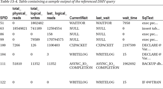
In this example, the database server is rebuilding a clustered index, running some long-running stored procedures with complex logic, deleting data from a table with blobs in them, and backing up a large database. Some of these tasks require a significant amount of I/O. As a result, you see in the wait types that the wait type for the backup SPID (111) is ASYNC_IO_COMPLETION, which is SQL Server waiting for an I/O completion event. SPID 104 and 122 are actually of more concern because they are waiting for their respective data to be committed (written) to the transaction log. In this event, it would have been wise to not run backups and stored procedure calls known to have high I/O while rebuilding a clustered index.

Figure 13-5 shows the quantity of bytes per second read and written and the response time to the SAN. As you can see, the response time ranges from 11 to 27 ms. In this environment, that’s a very long time. Coupled with the query results from Table 13-4, it illustrates that the server was very busy during this time.

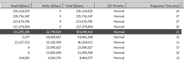
Figure 13-5. Illustration of server activity on a SAN under load.

In the result set, it’s helpful to know exactly what this query was doing. With that information, you can begin to dig deeper into your specific environment and address the I/O contention on two fronts: hardware and software (T-SQL). From here, you can choose to tune a particular query or take a broader view and interrogate the system tables about which indexes might be driving your I/O.

The following query provides usage statistics for your indexes:

This data set can help narrow down which of the tables in the query or stored procedure returned is the most or least used. Additional overhead could be due to a missing index, a fragmented index, index scans, or RowID lookups (bookmark lookups).

Another interesting query can be found by interrogating the sys.dm_os_schedulers object like this:

Unlike the previous queries in the chapter, the results of this query are solely based on current activity and do not represent historical data.

Addressing a Query

What you’ve just gone through can produce a lot of data, perhaps an overwhelming amount. However, perhaps you found that there’s a particular query that is the most expensive from an IO perspective. Perhaps you opened this chapter with one already in mind. The question is, how to address it. Before that however, you first must understand some characteristics around this query.

There are many good books on execution plans and I’m not going to spend time in this chapter discussing them as there’s an alternate manner to evaluate physical reads for a specific query or T-SQL batch. By using the statement SET STATISTICS IO ON, you can view some valuable characteristics about where a query is obtaining its data (disk or memory).

The following query was written for the AdventureWorksDW2008R2 database:

The output of this query isn’t relevant, but if you click on the messages tab you should see something similar to the following:

This output shows us some very interesting items. If you focus on the results for physical reads and read-ahead reads, you can begin to figure out how to better optimize this query or the objects it’s pulling data from.

The most interesting result I see here is the second reference to the object FactInternetSales. It has a physical read count of 10 and read-ahead reads of 1,032. In total, 1,042 data pages were retrieved from disk and placed into cache to satisfy the query. That’s a lot of data for a result set of only 13 rows. Granted, there is a GROUP BY involved, so it needed more rows in order to satisfy the WHERE clause, which alone returns 2,230 records.

So the question is, how can you make this query better with this data alone? If I run the statement sp_help FactInternetSales, part of the output for reads looks like Figure 13-6.

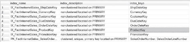
Figure 13-6. Illustration of the output of sp_help FactInternetSales.

This alone tells me that the query optimizer might try to use the index IX_FactInternetSales_ProductKey to satisfy the WHERE criteria, and it will most certainly use the clustered index PK_FactInternetSales_SalesOrderNumber_SalesOrderLineNumber. At this point, it doesn’t matter which one it’s using because I’m certain that, based on the columns in the index, the clustered key is where the majority of reads are coming from.

What if you took the simplest route with this query and simply added a covering index? A covering index is an index that satisfies the WHERE criteria and the join criteria, as well as the select columns in the query.

The index creation statement looks like this:

With that in place, the STATISTICS IO output for the query is as follows:

That’s much better. The count of pages necessary for the same query with that index in place dropped from a total of 1,042 to 11.

If this was a frequently run query, the potential IO savings are significant, as well as the potential memory savings. Instead of placing 1,302 pages of the table into memory, this query had a read-ahead count of only 8 pages.

To take it one step further, what if this index were compressed via row compression? This is a bit of a challenge because this table is relatively small and the dataset you are after is also small, but let’s see what happens.

An index can be rebuilt and row compression can be added in the following manner:

When the query is re-run, the STATISTICS IO output reads as follows:

It did help—a little. The total physical reads counter decreased from 3 to 2, but the logical reads (memory) decreased from 17 to 10. In this case, it had a minor impact on phsyical I/O but a more noticeable impact on memory I/O.

Additional resources for SET STATISTICS IO ON can be found at http://msdn.microsoft.com/en-us/library/ms184361.aspx. If you aren’t familiar with this option, I recommend reading up on it and adding it to your tool box. More information on read-ahead reads can be found at http://msdn.microsoft.com/en-us/library/ms191475.aspx.

With the simple statement SET STATISTICS IO ON, a very valuable set of data can be obtained about how SQL Server is trying to access your data and that statement will also point you to which object to focus on in a specific query.

Environmental Considerations

Earlier in this chapter, I mentioned a number of variables that come into play and will vary widely, even in your own environment. This portion of the chapter will cover the more common variables at a high level.

Depending on the version of the operating system and SQL Server, granting access to “Lock Pages in Memory” for the SQL Server service account will prevent the operating system from paging data in SQL Server’s Buffer Pool. This can have a marked impact in your environment. In my experience, I’ve seen this most often with virtualized SQL Server instances.

Another setting that can improve I/O throughput is “Perform volume maintenance tasks.” This permission allows the SQL Server process to instantly initialize files, which at start-up will decrease the time it takes to create TempDB. It also helps during incremental data-file growths or when new databases are being created. Note that this setting does not have an impact on transaction logs—only data files qualify for instant (zero fill) initialization.

I’ve discussed SANs at length in this chapter and, although the technology is continually changing, there are a couple of primary considerations to be aware of. The first is how the cache is configured on the controller. Typically, SANs contain memory, which is often backed up by battery power and enables that memory to be used as a write store. In this manner, your transactions won’t have to wait for the data to actually be persisted to disk. Instead, the data makes its way through the server, the host bus adapter (HBA), and then the controller. Depending on the specific SAN vendor, controller, and configuration, it’s likely that your data is only written to memory and then later flushed to physical spindles. What’s important here is how the memory is configured in your environment. Many vendors have an auto-balance of sorts, but for traditional database workloads the primary usage of cache is best used in a high-write configuration. For instance, if your controller has 1 GB of memory, it’s preferred, from a database workload, that the majority of that cache be allocated to writes rather than reads. After all, your database server has memory for read cache, but it does not contain write cache.

Another closely related setting to this is the queue depth on your HBA card. This is the piece of hardware that enables the server to connect to your SAN. The recommendations for configuring the HBA card vary and are based on your specific card, SAN, server, and workload. It’s worth noting, though, that increasing the queue depth can improve performance. As with anything of this nature, ensuring that you test your specific environment is critical. The good news, at this point, is that you have known IOP characteristics in hand about your environment and you can use these to configure a test with SQLIO. This utility measures your disk throughput and can be configured for the type of I/O you are interested in testing (read or write), the number of threads, the block size in KB (IOP size), among many other factors. It will test contiguous reads and/or writes and random reads and/or writes. Running this is intrusive to your disk subsystem—don’t run it in the middle of your business day. If you run this test, modify your queue depth, and then run it again, you can find the ideal balance for your specific workload on your specific hardware. The download for this can be found here: http://www.microsoft.com/en-us/download/details.aspx?id=20163.

Considerations about your I/O workload differ when working with virtual environments because the operating system is often running on the same set of spindles as your data files. These additional considerations can present opportunities for you to work with your virtualization expert and your storage guru to perhaps isolate the I/O required for the operating systems in the environment from your database files. A good way to illustrate the I/O required is with the Performance Monitor data discussed earlier and by using the SQLIO tool I just discussed.

Features of SQL Server will also impact your I/O. A great example of this is backup compression. When you use backup compression, fewer I/O requests are required to write the data file because it’s compressed in memory before it writes to the disk. Another SQL Server feature is Snapshot Isolation, which enables SQL Server to use optimistic locking rather than the default pessimistic locking scheme. The difference is considerable. Pessimistic locking can be considered serialized, meaning that modifications can occur for only one column at a time. With optimistic locking, Microsoft introduced a way for multiple requests to modify the same column. The reason that it’s important in this context is that the row version store required for Snapshot Isolation is in the TempDB database and can use TempDB aggressively, thereby increasing your I/O footprint. Again, this is an excellent feature, but one that must be tested in your specific environment.

Over the past several years, a few companies have risen to the forefront of I/O performance. I’ve had the pleasure of working with products from Fusion-io that provide very fast I/O throughput. I’ve used Fusion-io cards for TempDB, file stores, and even transaction logs. The throughput you can achieve with a Fusion-io card far exceeds that of traditional spindles, but the real value comes from the decreased latency. The latency of their entry-level product is measured in microseconds. This is pretty impressive considering that you measure I/O time in milliseconds. If you are considering purchasing this product or have a product similar to this, data files that require ultra-low latency benefit from this type of storage.

Compression is another feature that can benefit your I/O throughput and overall database performance, as it relates to I/O. There are two primary types of compression to be aware of. The first is backup compression. When creating a backup, you can choose to compress the backup. This decreases the amount of data that has to be written to disk. The second is data compression. Data compression comes in two primary forms: row and page. Chapter 14 dives into the details of data compression, but what you need to know for the purpose of this chapter is that data compression, if applied correctly, can significantly increase your database throughput, decrease your latency (read and write time), and improve the response time of your database server. It can also decrease memory pressure that you might be experiencing. There are many caveats to the case for using data compression and deciding which tables and index to compress in which fashion is critical. So be sure that you read the chapter on this topic and that you spend time to test.

Partitioning is another excellent avenue for decreasing your IOPS. Partitioning, in a nutshell, is akin to breaking your table up into many different tables. A quick example of this will help you understand the value of partitioning and, more importantly, the concept of partition elimination.

A simple illustration with the Transactions table that has a TransactionDate column will help. In this table, let’s say that you have one million records ranging from 2005 to 2010 (five years). For the purpose of this example, assume that the data distribution across each year is identical. For each year, there are 250,000 transactions (rows). When you run a query similar to SELECT COUNT (*), Convert(date, TransactionDate) as TransactionDate FROM Transactions where TransactionDate BETWEEN ‘06/01/2005’ and ‘06/01/2006’, the database engine will need to access n pages at the root and intermediate levels.

If partitioning is implemented on this table—specifically, on the TransactionDate column—you can decrease the footprint of the data that SQL Server needs to evaluate your particular query. Another way to think about this partitioning concept is akin to one of having multiple tables which contain the data in the Transaction table.. In this example, if you had a Transactions table for each year, SQL Server’s work would be significantly less. It would also make for some challenging T-SQL or implementation of a distributed partition view (DPV), but let’s keep it simple and just partition the table and allow SQL Server to eliminate what it doesn’t need to read. There are many good resources available to learn more about this subject, and one of my favorites can be found here: http://msdn.microsoft.com/en-us/library/dd578580(v=sql.100).aspx. Details specific to SQL Server 2012, including a change from previous versions of SQL Server as it relates to the quantity of partitions a table can contain, can be found here: http://msdn.microsoft.com/en-us/library/ms190787.aspx.

Conclusion

At times, there are no easy answers for dealing with the increase in data volumes that many of you experience on a daily basis. However, there are tools at your disposal to help you define and then articulate your specific situation. There are also design considerations you can help introduce or implement in your environment. It all begins with knowing your IOP pattern and being able to discuss it at a moment’s notice. Then work on the ideas you have gleaned from this chapter. Your IOP pattern will change over time and with new features and functionality. Keep your IOP profile up to date, take your storage guru out to lunch, build the bridge of communication and trust with your peers. Before you know it, you will be able to look this 800-pound I/O gorilla in the eye and not blink.