CHAPTER  4

Dynamic Management Views

By Kellyn Pot’vin

I’ve been working with Microsoft SQL Server since version 6.5 and was introduced to performance tuning and high-intensity database management in SQL Server 7 back in 2000. The environment at that time was a SQL Server 7 implementation clustered on a Compaq SAN and pulling in 1to 4 gigabytes (GB) per day, which was considered a great deal for a SQL Server back then. Performance tuning incorporated what appeared as voodoo to many at this time. I found great success only through the guidance of great mentors while being technically trained in a mixed platform of Oracle and SQL Server. Performance tuning was quickly becoming second nature to me. It was something I seemed to intuitively and logically comprehend the benefits and power of. Even back then, many viewed SQL Server as the database platform anyone could install and configure, yet many soon came to realize that a “database is a database,” no matter what the platform is. This meant the obvious-: the natural life of a database is growth and change. So, sooner or later, you were going to need a database administrator to manage it and tune all aspects of the complex environment.

The days of voodoo ceased when SQL Server 2005 was released with the new feature of Dynamic Management Views (DMVs). The ability to incorporate a familiar, relational view of data to gather critical system and performance data from any SQL Server version 2005 or newer was a gigantic leap forward for the SQL Server professional. As an Oracle DBA who had access to V$* and DBA_* views for years, the DMV feature was a wonderful addition to Microsoft’s arsenal of performance tools.

In this chapter, I will not just describe the views and how to collect the data, but I’ll cover why collecting this data is important to the health and long performance of an MSSQL database. Performance tuning is one of the areas that I see often neglected in MSSQL, because it is often marketed as being easy to set up, yet it takes strong, advanced database knowledge to understand what can hinder performance and how to resolve that problem. The introduction of Dynamic Management Views gives you the ability to provide clear, defined performance data, whereas before they were introduced, incorrect assumptions were easily made and many mistakes resulted from them.

Understanding the Basics

Dynamic Management Views must be used with Dynamic Management Functions (DMFs). There is no way around this: the views are the data, and the table functions offer you the additional processing capability required to view the data—specifically, using the OUTER and CROSS APPLY operators to present the results in a proper format for easy readability.

Table functions can perform more than a single select (that is, of a view). When that functionality is used with Dynamic Management Views, it offers more powerful logic choices than any view alone could offer.

Before you can use the techniques found in this chapter, you need to understand basic database administration, which includes knowing how to locate a database ID (DBID), how to query views with function calls, and the differences between SQL calls from Procedure object names.

Naming Convention

The DMVs and DMFs reside in the SYS schema and can be located by their specific naming convention of dm_*. No aliases (synonyms) have been created for DMVs or DMFs, so you must prefix them with the sys. schema name. When DMVs are discussed, they often are referred to with the sys. in the name, but within this chapter, the sys. part will be assumed—for example, sys.dm_exec_sql_text.

These naming conventions can be confusing at times, depending on what type of dynamic-management object you are referring to. DMVs can be queried using a “simple” naming convention, whereas DMFs can be referenced only with the standard two-part and three-part names—that is, <dbname>.<dbowner>.<view_name>, not the four-part, fully qualified naming convention, which adds the <dbserver> prefix.

For example, if you want to query the Employee table from the HumanResources schema in the AdventureWorks2012 database that resides on ServerHost1, the naming convention breakdown looks like the following:

• Four-part ServerHost1.AdventureWorks2012.HumanResources.Employee
• Three-part AdventureWorks2012.HumanResources.Employee
• Two-part HumanResources.Employee

Groups of Related Views

More views and functions have been added in each subsequent SQL Server release to support the dynamic-management features. These views are then grouped by usage. In SQL Server 2005, there were 12 initial groups; in 2008, there were 15; and in 2012, there are now 20 groups of views. These additional groups include ones to support the new disaster-recovery and high-availability feature: the AlwaysOn Availability Groups Dynamic Management Views and Functions group.

As of 2012, the DMVs are broken down into the following groups:

• AlwaysOn Availability Group Dynamic Management Views and Functions
• Index Related Dynamic Management Views and Functions
• Change Data Capture Related Dynamic Management Views
• I/O Related Dynamic Management Views and Functions
• Change Tracking Related Dynamic Management View
• Object Related Dynamic Management Views and Functions
• Common Language Runtime Related Dynamic Management Views
• Query Notifications Related Dynamic Management Views
• Database Mirroring Related Dynamic Management Views
• Replication Related Dynamic Management Views
• Database Related Dynamic Management Views
• Resource Governor Dynamic Management Views
• Execution Related Dynamic Management Views and Functions
• Security Related Dynamic Management Views
• Extended Events Dynamic Management Views
• Service Broker Related Dynamic Management Views
• Filestream and FileTable Dynamic Management Views (Transact-SQL)
• SQL Server Operating System Related Dynamic Management Views
• Full-Text Search and Semantic Search Dynamic Management Views
• Transaction Related Dynamic Management Views and Functions

To query DMVs and DMFs, the user must have the VIEW SERVER STATE or VIEW DATABASE STATE permission granted. Without this permission, users receive an error stating the object does not exist.

Varbinary Hash Values

To query the data from a DMV, you need to use SQL Server’s version of a system-generated hash value, called the handle. The handle replaces other options that could have been used but would have been more difficult, including data that is stored in XML formats. A handle is stored in a varbinary(64) datatype, and the performance benefits for doing this are apparent.

Varbinary is variable-length binary data. A varbinary value can be a value from 1 to 8,000. After creation, when measuring allocation, the storage size is the actual length of the data entered plus an additional 2 bytes.

Following are some characteristics of varbinary data:

• Varbinary is data that has inconsistent or varying entries.
• Varbinary is more efficient if any sorting is required because it does not require collation.
• Varbinary generally consumes fewer bytes on average than a varchar or other common datatype choices.
• Note that, as different datatypes are converted to varbinary, they can be padded or truncated on the left or right, depending on the datatype they are being converted from.

The two most widely used varbinary datatypes in DMVs are the following:

• plan_handle  Hash value of the execution plan for the sql_handle in question.
• sql_handle  Hash value of a given SQL statement. This is a unique value for a SQL statement that is produced by an algorithm that will guarantee that the same sql_handle will appear on any SQL Server server for a unique statement. This can be very useful in clustered environments or for comparisons between development, test, and production SQL Server servers.

You will find that there are a number of ways to query the sql_handle. The following code demonstrates how to pull the sql_handle for a procedure call:

The following code shows how to query the handle with a select command, with the results shown in Figure 4-1:

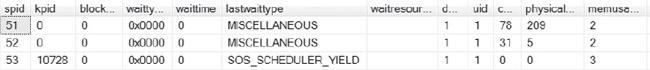
Figure 4-1. Results joining sys.processes and sys.dm_exec_sql_text.

Each SQL Server performance-tuning DBA has its own suite of scripts to query DMVs in times of performance challenges. Included in this chapter is my own collection of scripts that I have pulled together through the years. Most of them are sourced from MSDN, various websites, and books. I made changes to some of them as was required for the environment I was working in, but I’ve often noticed that many DBAs query the data the same way to gather the same pertinent information.

Common Performance-Tuning Queries

Performance tuning is an area that many have found more difficult to master in SQL Server than they might have in other database platforms. The DMVs covered in this section represent an incredible leap in the direction of performance control, understanding, and reporting that the SQL Server DBA didn’t have access to in earlier days.

Because performance tuning is my niche, the *exec* DMVs are by far my favorite area of the featured DMVs. This section covers how to locate connection, session, and status information, and then moves on to actual query stats and performance metrics.

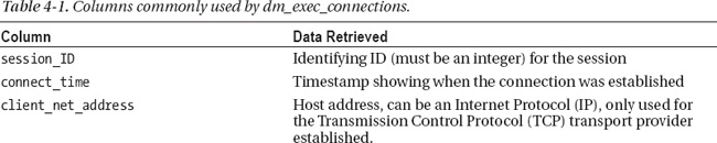
Retrieving Connection Information

Query the sys.dm_exec_connections view to retrieve information about connections to the database. Table 4-1 lists the most commonly used columns in the view.

Following is an example query against the view. The query returns a list of current connections to the instance.

Figure 4-2 shows my output from this query.

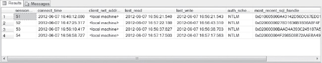
Figure 4-2. Example output showing currently connected sessions.

Showing Currently Executing Requests

For the dm_exec_requests DMV, the results show information about each of the requests executing in SQL Server at any given time. The results from this view will appear very similar to the sp_who view of years gone by, but the DBA should not underestimate the added value of this DMV.

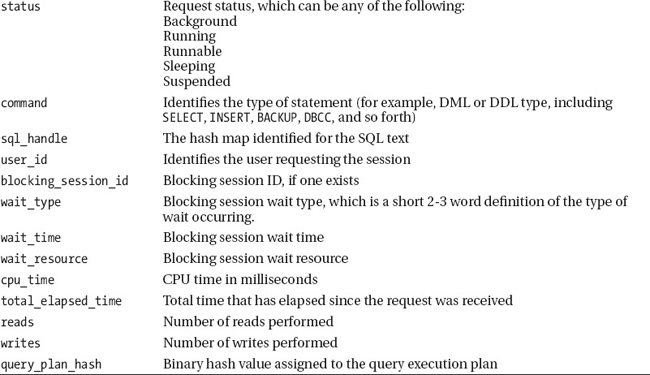
Table 4-2 lists columns commonly used in this view.

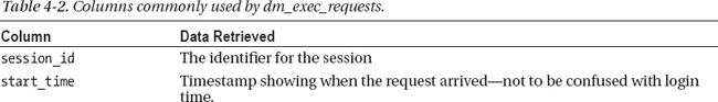
The dm_exec_requests DMV can pull basic information or be joined to other views, such as dm_os_wait_stats, to gather more complex information about sessions currently executing in the database. Here’s an example:

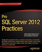
Figure 4-3 demonstrates the output for the current requests.

Note that the background processes for MSSQL, (the session number is less than 51, which signifies a background system session) are displayed with the command type and purpose, along with what database (DBID) it belongs to.

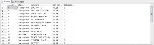
Figure 4-3. Example output showing current requests.

Locating a blocked session and blocked information is simple with sys.dm_exec_requests, as the following example shows:

Figure 4-4 shows an example of results for a blocked session.

Figure 4-4. Example output showing a blocking session.

In the scenario shown in Figure 4-4, you can see that the blocked session (56) is blocked by session ID 54 on an update for the same row (LCK_M_U), and that it is suspended until the lock is either committed or rolled back. You now identify the transaction_id, which can also be used for further information in joins to secondary DMVs.

Locking Escalation

Locking escalation is one of the enhanced features in SQL Server that Microsoft spent a lot of time on. When an issue does arise, it is important that the DBA understand what is occurring and how to address a lock-escalation issue. If you do experience a locking issue in one of your databases, the following query, using the dm_trans_lock DMV returns information regarding locking status from the database in question.

Figure 4-5 shows the results of this query.

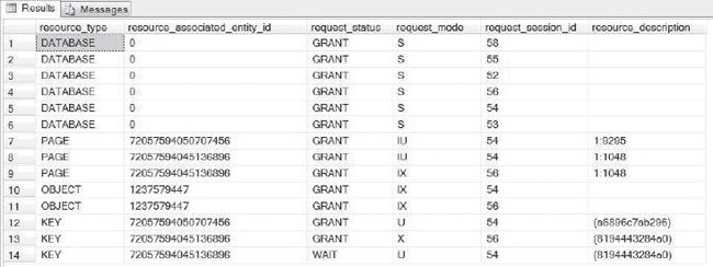
Figure 4-5. Demonstration of locking-escalation information shown in SQL Server.

In Figure 4-5, you can see that there is a lock escalation in progress between session IDs 54 and 56. The “Page” escalation on resource_associated_entity_id (the Employee table) involves the index (IX, KEY) as well. Always be aware of object and key escalations. Lock escalation should work seamlessly in SQL Server and when issues arise, always inspect the code and statistics first for opportunities for improvement.

Identifying what type of locking status, including, the mode, the transaction state the lock is in, addressing a lock that has escalated and has created an issue are pertinent parts of the DBA’s job. Gathering the information on locking is now simple—you do it by joining the dm_tran_locks DMV to the dm_os_waiting_tasks DMV, as shown here:

Finding Poor Performing SQL

As a performance-tuning DBA, I find the DMVs in the next section to be some of my favorites. These DMVs are the most commonly queried by any DBA looking for performance issues with the plan cache of SQL Server. With these queries, you can view aggregated data about execution time, CPU resource usage, and execution times.

How is this view an improvement over the voodoo that DBAs used to perform to locate issues in versions of SQL Server prior to 2005?

• It isolates each procedure and procedure call to identify how each one impacts the environment. This can result in multiple rows for the same procedure in the result set.
• It immediately isolates an issue, unlike the SQL Profiler.
• It produces impressive results when you use it with the DBCC_FREEPROCCACHE before executing queries against it.
• It can be used to create performance snapshots of an environment to retain for review when performance issues arise.
• It makes it easy to isolate top opportunities for performance tuning, allowing the DBA to pinpoint performance issues—no more guessing.
• Not all queries show up in this view. SQL that is recompiled at the time of execution can circumvent the view results. (You need to enable StmtRecompile to verify.)
• It can be used with a multitude of SQL Server performance tool suites (such as DB Artisan, Performance Dashboard, Toad, and so forth). However, these tools might not give you the full access that querying the view might grant to a DBA.

Here is what happens when performance data with DMVs isn’t 100 percent accurate:

• Removing the compiled plan from cache will result in the corresponding rows for the query plan being removed from the DMV as well.
• Results will show in this DMV only after the query execution has successfully completed, so any SQL that is still executing or long-running queries can be missed because of this fact.
• Cycling the SQL Server or any interruption in service to the hardware will remove the corresponding rows from the DMV as well.

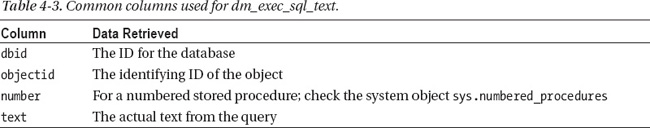
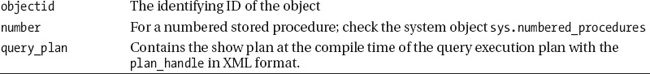
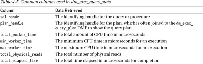
The most common method of locating performance issues with SQL is by using the dm_exec_sql_text, dm_exec_query_plan, and dm_exec_query_stats DMVs, which are joined together to give DBAs the most accurate information about the database. Tables 4-3 through 4-5 list the columns most commonly used of these DMVs.

Using the Power of DMV Performance Scripts

Locating the top 10 performance challenges in any given database can be a powerful weapon to use when issues arise. Having this data at your fingertips can provide the DBA, developer, or application-support analyst with valuable data about where to tune first to get the best results.

There are two areas in this query, along with the subsequent ones in this section, that I want you to fully understand. The first is the initial column of SQL, followed by the XML output of the showplan, which you can see in Figure 4-6.

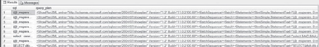
Figure 4-6. Top 10 performance-challenging queries, arranged by total working time in the database.

The example in Figure 4-6 shows the results of a CPU intensive environment. As helpful as this data is, the process of collecting this data can add CPU resource pressure to a production environment and the database professional should take care regarding when and how often this type of query is executed. The benefits of the resulting query are the links shown for the show plan data, which can then be clicked on to show the full SQL for the statement in row chosen.

When investigating further, the next area of focus is on how the quantity of execution counts corresponds to the impact to CPU, reads, durations and other pertinent data, as shown in Figure 4-7.

Figure 4-7. The response from this query results in a wide array of columns that can then identify SQL code with high execution counts, extensive physical reads and/or elapsed time.

When any performance DBA is evaluating easy options for performance tuning, identifying the low-hanging fruit—that is, comparing the number of executions to the time they take and the impact they have on the CPU—is crucial. Identifying and tuning these can result in a quick performance gain  by making small, efficient corrections to one to five offending top processes rather than creating a large, resource-intensive project to correct an environment.

Note also that the preceding queries and subsequent ones all have a common DMF call in them. You can use this DMF to retrieve a sql_handle for a given SQL statement, such as CROSS APPLY sys.dm_exec_sql_text(sql_handle) sql. As mentioned earlier, for performance reasons DMVs refer to SQL statements by their sql_handle only. Use this function if you need to retrieve the SQL text for a given handle. This DMF accepts either the sql_handle or plan_handle as input criteria.

Many of the performance DMFs won’t complete in SQL Server environments if version 8.0 (SQL 2000) compatibility is enabled. The common workaround is to execute the DMF from a system database using the common fully qualified name—for example, CROSS APPLY <dbserver>.<dbname>. sys.dm_exec_sql_text(plan_handle).

Divergence in Terminology

Terminology divergence is a common issue for many as new versions and features evolve. Note that DMVs that use the plan handle to execute results within the execution plan will also be referred to as the showplan. This now is often shown as a link in a user-friendly XML format. The links will only display plans that are executed or are still in cache. If you attempt to display plans other than these, a null result will occur upon clicking on the link.

• Execution plans in XML format are often difficult to read. To view execution plans graphically in Management Studio, do the following:
  • The function will return a hyperlink automatically for the showplan XML.
  • Click on the hyperlink to bring up the XML page in an Internet browser.
  • Click on FileSave As and save the file to your local drive using a .SQLPLAN file extension.
  • Return to SQL Server Management Studio. You can now open the file you just saved without issue.
• It is a best practice to retain an archive of the XML for execution plans of the most often executed SQL in each environment.
• The creation of XML for any execution plan uses a fair amount of CPU. I recommend performing this task at off hours if you are executing the XML on a production system.
• You can use the data in the show plan for comparisons when performance changes occur, allowing you to compare performance changes and pinpoint issues.
• The query plan is based on the parameters entered during the execution of the first query. SQL Server refers to this as parameter sniffing. All subsequent executions will use this plan whether their parameter values match the original or not.
• If a poor combination of parameters was saved to the base execution plan, this can cause performance issues not just for the original execution but for all subsequent ones. Because you can view this in the execution-plan XML, knowing how to view this data when you have concerns regarding a query can be very helpful.
• If you do suspect an issue, you can locate the correct plan and force its usage with the OPTIMIZE FOR hint.

Optimizing Performance

There are many versions of queries joining the DMVs dm_exec_query_stats and dm_exec_sql_text to provide a DBA with information regarding poor performance. The following is a collection of queries that I retain in my own arsenal to locate and troubleshoot performance.

Top 1000 Poor Performing is a script that will generate a large report, showing the worst code executed in the environment, and for many environments, it will show some of the least offending code executed in the environment. This provides you with a solid understanding of what code is executed in the environment and how much is high impact and how much is standard processing and everyday queries.

When you execute this query, it returns the top 1000 procedures or processes and it breaks down performance impacts by the actual procedural calls, listing the offending code from the procedure or complex process, as Figure 4-8 shows.

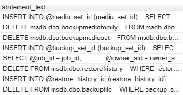
Figure 4-8. Results of the top 1000 SQL Statement text from the query.

You can also take advantage of various joins between dm_exec_query_stats and dm_exec_sql_text to clearly identify the statement by average CPU and SQL text, two of the most important aspects to note when researching poorly performing SQL. Here’s an example:

The results are shown in Figure 4-9.

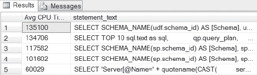
Figure 4-9. The top five offending statements, ordered by average CPU time. This query is based on the “top 20,” which results in a more defined report for the DBA to inspect and clear CPU-intensive resource data that is important in terms of performance.

Always remember, CPU is everything in a SQL Server environment. The output from many of the performance queries in this section of the chapter gives the DBA a clear view of what statements are the largest impact on this important resource usage.

The results of this query are shown in Figure 4-10.

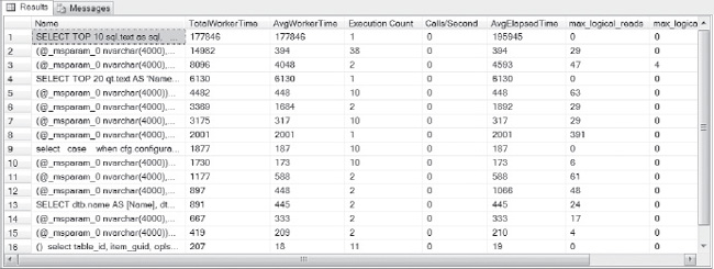
Figure 4-10. CPU usage, time, and reads, broken down by averages, minimums, and maximums.

Inspecting Performance Stats

Generating useful performance stats have been a common challenge for SQL Server DBAs. DMVs offer another option for extracting information that provides clear answers that can then be viewed in a user-friendly XML format.

Performance statistics can come in many forms- physical reads, logical reads, elapsed time and others. The following query is an excellent demonstration of high-level performance statistics in a MSSQL environment.

Figure 4-11 shows the results of this query.

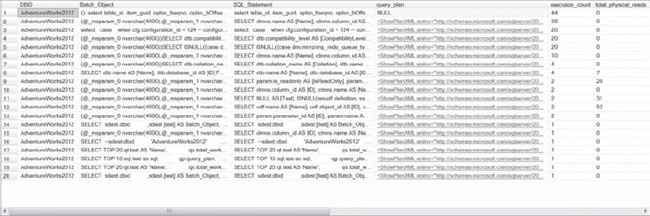
Figure 4-11. XML query plan links offered through DMVs that open a browser to the showplan for each statement and provide more defined performance data.

Top Quantity Execution Counts

As any performance-oriented DBA knows, it’s not just how long a query executes, but the concurrency or quantity of executions that matters when investigating performance issues. DMVs provide this information and, in more recent releases, inform you of how complete the data is with regard to concurrency issues, which can be essential to performing accurate data collection.

The results of this query are shown in Figure 4-12. They show that a process has performed a full scan on the HumanResources.employee table 10,631 times, and they show the average worker time, average elapsed time, and so forth.

Figure 4-12. Highly concurrent SQL; note the average elapsed time versus. the number of executions shown in the Execution Count column.

Physical Reads

Another area of high cost to performance is I/O. Having a fast disk is important, and as SQL Server moves deeper into data warehousing, having a faster disk and fewer I/O waits are both important to performance. There is a cost to all reads, regardless of whether they are physical or logical, so it is crucial that the DBA be aware of both.

The results of this query are shown in Figure 4-13.

Figure 4-13. Physical and logical read data generated by the preceding query.

Physical Performance Queries

Physical performance tuning involves indexing, partitioning and fragmentation unlike the queries in the previous section, which are often used to discover opportunities for logical tuning.

Locating Missing Indexes

When SQL Server generates a query plan, it determines what the best indexes are for a particular filter condition. If these indexes do not exist, the query optimizer generates a suboptimal query plan, and then stores information about the optimal indexes for later retrieval. The missing indexes feature enables you to access this data so that you can decide whether these optimal indexes should be implemented at a later date.

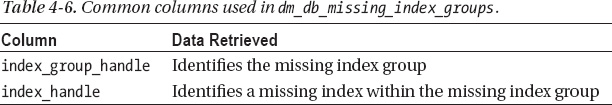
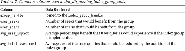
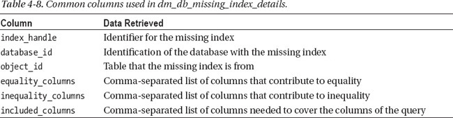
Here’s a quick overview of the different missing index DMVs and DMFs:

• sys.dm_db_missing_index_details (DMV)  Returns indexes the optimizer considers to be missing
• sys.dm_db_missing_index_columns (DMF)  Returns the columns for a missing index
• sys.dm_db_missing_index_group_stats (DMV) ; Returns usage and access details for the missing indexes similar to sys.dm_db_index_usage_stats.

The pertinent columns for these three DMVs and DMFs are covered in Tables 4-6 through 4-8.

For these DMVs to be useful, the SQL Server instance must have been in service for a solid amount of time. No set amount of time can be given, because the level of knowledge of the database professional’s is what determines whether sufficient processing has occurred to provide the DMVs with accurate data. If the server has just been cycled, you will be disappointed with the results. The only way SQL Server can tell you if indexes are used or missing is if the server has had time to collect that information.

Take any recommendations on index additions with a grain of salt. As the DBA, you have the knowledge and research skills to verify the data reported regarding index recommendations. It is always best practice to create the recommended index in a test environment and verify that the performance gain is achieved by the new index. Indexes should always be justified. If you create indexes that are left unused, they can negatively impact your environment, because each index must be supported for inserts and updates on the columns that they are built on.

Identifying missing indexes to improve performance is a well-designed and functional feature that DMVs offer. Note that the index recommendations that are needed are collected during the uptime of the database environment and are removed on the cycle of the database server. There is a secondary concern that needs to be addressed. Is this is a test environment or a new environment, where processing would not have accumulated the substantial time required to offer valid recommendations? Information must be accumulated in the DMV to provide accurate data, so a nonproduction or new environment might yield inaccurate results.

The above query will only result in accurate results if you first run the Database Engine Tuning Advisor fromtheManagement Studio to determine your initial indexing needs. The simple wizard will take you through the steps needed to easily execute the analysis, and it will locate the new object readily, as shown in Figure 4-14.

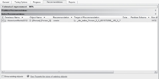
Figure 4-14. Results of the Database Engine Tuning Advisor.

Index performance challenges involve determining how the index is used and whether there is an index for a specific query to use. Reporting aggregated totals for all index usage in the current database—broken down by scans, seeks, and bookmarks—can tell you if your indexing is efficient or if changes are required. By using the dm_db_index_usage_stats DMV, you can find out exactly how an index is used. In the view, you will see the scans, seeks, and bookmark lookups for each index.

Removing unused indexes produced some of my largest performance gains in most SQL environments. It is common for many to mistakenly believe “If one index is good, more means even better performance!” This is simply untrue, and as I previously stated, all indexes should be justified. If they are unused, removing them can only improve performance.

Index usage should be established over a period of time—at least one month. The reason for this is that many environments have once-per-month or month-end processing, and they could have specific indexes created for this purpose only. Always verify the index statistics and test thoroughly before dropping any index.

You will know the index is unused when all three states—user_seeks, user_scans, and user_lookups—are 0 (zero).

Rebuild indexes based on the value in dm_db_index_usage_stats. Higher values indicate a higher need for rebuilding or reorganizing.

Return all used indexes in a given database, or drill down to a specific object. Remember that the following query returns only what has been used since the last cycle of the SQL Server instance.

Additionally, with a small change, using very similar columns to the dm_db_ missing_index_group_stats view, you now have view results based on index usage rather than the results you got from previous queries, which focused on indexes that were missing:

Figure 4-15 shows the results from the preceding query and that the Person_2, Employee, and Department tables are experiencing full scans. It is important for the DBA to understand why the scan is being performed. Is it due to a query, an update, or a hash join?

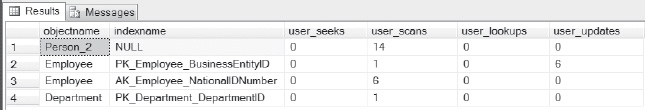
Figure 4-15. Table scans versus different types of index scans.

You can also use the missing views on indexing to view when you are not using an index. This is one of the most common tuning gains for a DBA: adding missing indexes to avoid table scans.

Figure 4-16 shows the results of this query.

Figure 4-16. Tables without indexes.

As I stated before, locating unused indexes and removing them can be one of the quickest ways a DBA can produce performance gains, as well as achieve space-allocation gains. Executing the following query will join the dm_db_index_usage_stats DMV to sys.tables and sys.indexes, identifying any unused indexes:

Figure 4-17 shows the results.

Figure 4-17. Unused index on table Person.

The index shown in Figure 4-17 was created by me for just this query. It’s never been used and is on the column MiddleName of the Persons table. This might seem like a ridiculous index, but it would not be the worst I’ve identified for removal. The important thing to note is that you should monitor unused indexes for at least a month’s time. As new objects and indexes are placed into an environment, they might not be called (that is, objects are released, but application code is to be released at a later date that will call upon the index, and so forth). These scenarios must be kept in mind when choosing indexes to remove, because removing a needed index can have a serious performance impact to the users or applications.

Partition Statistics

Reporting on partition statistics can offer the DBA pertinent day-to-day data storage information, performance information, and so forth. Knowing how to join to system tables, such as sys.partitions, is important because it can give database professional more valuable data, as well as reviewing space usage and LOB info.

The DMVs will show only one row per partition. This allows the DMV to simplify partition count queries for any given object. Row overflow data, which is extremely important to maintenance work, can be pulled easily from the DMV, too.

Querying partition statistics DMVs offer high hit partitions with drill down lists, page and row-count information. The OBJECT_ID function can then be used to identify the objects from the views by name.

Retrieving information about used pages and the number of rows on a heap or clustered index can be challenging, but not if you use the following query:

Figure 4-18 shows the results.

Figure 4-18. Statistics on a partitioned index.

Locating partitions with the largest row counts can give you pertinent data about future partitioning needs. This data can be very helpful when deciding whether to create a subpartition.

The results are shown in Figure 4-19.

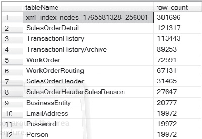
Figure 4-19. Row counts on partitions.

System Performance Tuning Queries

System requests are often joined with the operating system wait DMVs (referred to as operating system waits) to give DBAs a clear picture of what is occurring in a SQL Server environment. Where once the DBA was dependent on the information in sp_who and sp_who2, now they can use the information in DMVs and have defined control over the data regarding system information in a SQL Server environment.

What You Need to Know About System Performance DMVs

Any database professional will have an appreciation for the replacement DMV queries for sp_blocker and sp_who2. You can now request the blocking session_ids and locate issues more quickly, along with extended data with DMVs.

During joins to dm_exec_requests, always verify the blocking session_id. As with any time-sensitive views, you need to know that you have the most up-to-date information in your blocking session results.

Percent_complete and estimated_completion_time can now be retrieved for tasks such as reorganizing indexes, backing up databases, and performing certain DBCC processes and rollbacks In the past, this data was unavailable.

Keep in mind that the data used by the following queries doesn’t have to be cleared by a cycle of the database server or services. The data can also be cleared by running DBCC FREEPROCCACHE.

Sessions and Percentage Complete

Being able to track sessions and obtain information about the logged-in session (such as whether it’s active and, if so, how close to complete the process is) is a task most DBAs face daily. DMVs offer up this information in a simple, easy-to-read format, which is focused on the session ID and results that include the SQL statement text and the percentage complete:

Figure 4-20 shows the result of this query.

Figure 4-20. Locating all available requests with percentage complete.

The following query locates all active queries, including blocked session information:

Figure 4-21 shows the result of this query.

Figure 4-21. Locating all active queries, including blocked-session information.

The two DMVs—dm_os_tasks and dm_os_threads—can be joined to identify the SQL Server session ID with the Microsoft Windows thread ID. This has the added benefit of monitoring performance and returns only active sessions.

Figure 4-22 shows the results of this query.

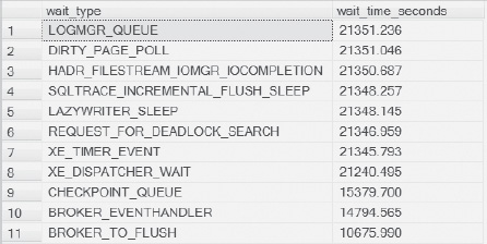
Figure 4-22. Results of query showing session_id and the matching operating system thread ID in Windows.

Of course, the most important session ID info most investigations need is the information for any session IDs less than 51.

Wait statistics are important in any database, and SQL Server is no different. The following DMV, dm_os_wait_stats, lists the wait type and also shows you the wait time in seconds. You’ll find this very useful when looking for the top five wait statistics in any given environment.

Figure 4-23 shows the results of this query.

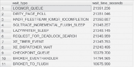
Figure 4-23. Results for different wait types in SQL Server.

In Figure 4-23, there isn’t any user processing, only background processes, so the wait time in seconds won’t be the standard event times you would normally see.

Gaining insights into which operating-system processes have issues is sometimes left to the DBAs perception and assumptions. The DMV dm_os_workers takes the guesswork out of this task by listing each of the operating-system sessions, indicating whether there is an actual issue with any one of them.

The results are shown in Figure 4-24.

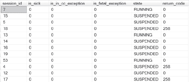
Figure 4-24. Health results of operating-system processes on the database server.

If any of the preceding processes were found to be in trouble (that is, they showed up as is_sick, is_in_cc_exception or is_fatal_exception), they would have returned a value of 1 in Figure 4-24. Here is a list of the values that indicate some sort of trouble:

is_sick	Process is in trouble
is_in_cc_exception	SQL is handling a non-SQL exception
is_fatal_exception	Exception has experienced an error

The meaning of the codes in the State column are as follows:

INIT	Worker is currently being initialized.
RUNNING	Worker is currently running either non-pre-emptively or pre-emptively.
RUNNABLE	Worker is ready to run on the scheduler.
SUSPENDED	Worker is currently suspended, waiting for an event to send it a signal.

And the meaning of the return codes are the following:

0	Success
3	Deadlock
4	Premature Wakeup
258	Timeout

The dm_os_volume stats view, which is new to SQL Server 2012, returns the disk, database-file, and usage information. There is no known way to collect this data for a pre-2012 version of SQL Server.

For my little test hardware, there isn’t much that’s interesting to report on (as you can see in Figure 4-25), but this data could prove incredibly valuable in production environments when you want to inspect the I/O resources available to the database server.

Figure 4-25. Volume stats of mount points obtained through the dm_os_volume stats DMV.

I included the transactional snapshot information because I find the virtual table generation an interesting feature of this view. It’s not commonly used, but it demonstrates how easy it is to use these views and produce valuable information from them.

The following query reports transactions that are assigned a transaction sequence number (also known as an XSN). This XSN is assigned when a transaction accesses the version store for the first time.

Keep the following in mind when executing this query:

• The XSN is assigned when any DML occurs, even when a SELECT statement is executed in a snapshot isolation setting.
• The query generates a virtual table of all active transactions, which includes data about potentially accessed rows.
• One or both of the database options ALLOW_SNAPSHOT_ISOLATION and READ_COMMITTED_SNAPSHOT must be set to ON.

The following is the output from executing the query:

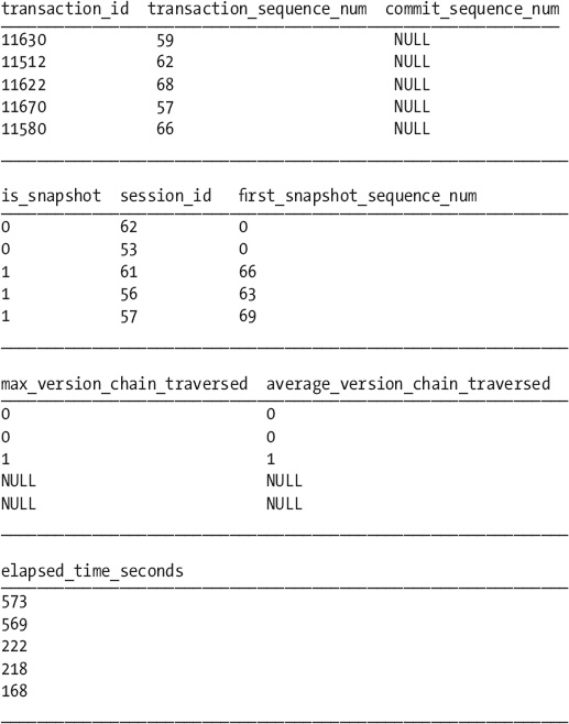
Here’s how to read these result tables:

• The first group of columns shows information about the current running transactions.
• The second group designates a value for the is_snapshot column only for transactions running under snapshot isolation.
• The order of the activity of the transactions can be identified by the first_snapshot_sequence_num column for any transactions using snapshot isolation.
• Each process is listed in order of the transaction_id, and then by elapsed_time.

Conclusion

Anyone database administrators who were troubleshooting performance-level or system-level issues before the existence of Dynamic Management Views faced unique challenges. The introduction of this feature has created a relational database management system environment with robust performance-tuning and system-metric-collection views that DBAs can use to figure out answers to the performance challenges that exist in their SQL Server environments.