
The preceding chapter dealt with graphics on a pixel-by-pixel basis, and this is fine for simple rendering. When you’re building a multilayered, multiplayer game, however, you need to program at a higher level. At the very least, you need to create graphics with three dimensions rather than two. This means dealing with concepts such as lighting, depth, and perspective. The functions in OpenGL (Open Graphics Library) make this possible.
Now is a giddy time to write about OpenGL, particularly for the Cell processor. As I write this, three tumultuous developments have either taken place recently or are underway:
The Khronos Group has announced the development of OpenGL 3.0, which promises to be completely different than OpenGL 2.1.
Brian Paul has released the open source Gallium toolset for 3D graphic development, a complete departure from the old Mesa toolset.
An OpenGL driver for the Cell is now available. Unlike regular Mesa drivers, it’s based on Gallium.
This presentation in this chapter consists of two parts. The first presents the history of OpenGL and explains the developments to come. The second part discusses the technical aspects of OpenGL development: creating a window with GLUT, defining a viewing region, and placing OpenGL graphics inside the viewing region.
To understand the upheavals that face OpenGL development, it helps to know something about its history. This brief treatment provides background on OpenGL, including its origin and purpose. It also introduces Mesa, the open source, hardware-independent implementation of OpenGL.
It’s been over fifteen years, but I can still remember the first time I saw the demonstration of Silicon Graphics’ Indigo workstation. The presenter talked about geometry and vectors and state machines, but no one paid attention: All we could do was stare hypnotized at the viewscreens. The graphic processing was light years beyond anything available at the time—higher speed and higher resolution than any console or computer. The years haven’t been kind to Silicon Graphics or the Indigo, but the graphic programming API, OpenGL, continues to evolve and find new adherents.
Put simply, OpenGL defines a set of functions that build graphical applications. These routines perform many tasks, including the following:
Identify vertices in two and three dimensions
Combine vertices into shapes (lines, triangles, rectangles, polygons)
Define colors and coloring schemes for the vertices and shapes
Manage the viewing scene with transformations and depth ordering
When Silicon Graphics (SGI) made OpenGL available to third-party licensees in the early 1990s, it became a great and popular success. Software programmers were happy because they had a standard, high-level means of building 3D applications. Hardware vendors were also happy because they knew what routines their graphics devices had to implement.
Until 2006, OpenGL development was overseen by the OpenGL Architecture Board (ARB). In addition to defining the standard set of OpenGL functions, the ARB created an extension mechanism for including vendor-specific features. For example, if a new graphics card from NVidia provided a capability that couldn’t be accessed in OpenGL, the ARB would add an NVidia-specific function to its list of approved extensions. As other vendors’ hardware implemented the new feature, the ARB might include the extension in the core API.
The OpenGL standard grew from version 1.0 in 1992 to version 2.1 in 2006. As graphics cards gained new features (antialiasing, texture mapping, anisotropic filtering), OpenGL gained new functions. Two problems arose. First, the ARB tended to deliberate slowly on new extensions. This made it difficult for developers to know whether specific hardware features would be accessible in code.
The second problem is that the API grew bloated, functions became redundant, and OpenGL code became harder to write and understand. Two developers might code similar OpenGL applications but use completely different sets of functions, and only trial and error could determine which set of functions operated faster.
SGI’s fortunes reached a nadir in 2006, and control of the OpenGL API passed to an organization called the Khronos Group. This group, headed by NVidia, Sun, Sony, Intel, and many other corporations, formed a second OpenGL ARB to manage OpenGL development.
At the SIGGRAPH conference in August 2007, the Khronos Group announced the development of OpenGL 3.0. Michael Gold from NVidia presented a number of planned changes, including streamlining the API and simplifying the process of building applications and drivers. He discussed a new object-oriented approach to graphics and stressed the importance of getting “back to the bare metal.”
As I write this in July 2008, no further technical information has been made available. While the Khronos Group has stayed silent, developers have been vocal in their concern. The OpenGL 3.0 forum at opengl.org contains over 120 pages of posts whose tone ranges from hopeful anticipation to utter despair.
In 1993, a graduate student named Brian Paul coded his own OpenGL implementation called Mesa. Mesa is a software implementation of OpenGL, which means that the API functions are processed by the CPU rather than dedicated hardware. This makes Mesa more portable than hardware-specific OpenGL implementations, but the performance is reduced significantly.
Thanks to the continued diligence of Brian and other developers, Mesa has stayed current as new features are added to OpenGL. It’s been ported to multiple operating systems and windowing systems, and it’s particularly important for Linux and the X.Org implementation of the X Window System. When a Linux application calls OpenGL routines, Mesa processes the functions and calls the appropriate X Window System functions.
Recognizing Mesa’s popularity, graphic card vendors have developed drivers that interface the Mesa libraries. These drivers enable OpenGL applications to bypass the X server and directly access the hardware. This bypass is made possible through the Direct Rendering Infrastructure (DRI). This is not currently possible for the PlayStation 3, whose NVidia hardware can’t be accessed by user applications.
In 2007, Brian Paul and his company, Tungsten Graphics, started work on a new architecture for their graphics software. The goal was to divide the processing tasks into modular components with simple interfaces. This way, the framework could support different classes of graphics hardware and different programming APIs, including Microsoft’s Direct3D. They called the project Gallium, and Figure 20.1 shows its software structure.
Mesa is still an important part of the Gallium framework, but serves mainly as a front end. It provides information about the graphic state to the State Tracker, which relays this information to the Gallium driver. The Gallium driver renders the graphics by interfacing the back-end processing elements. This may be a graphics card or an application that runs on the CPU.
This chapter’s primary concern is the driver for the Cell processor, shown at the bottom of the figure. This driver runs on the PowerPC Processor Unit (PPU) and renders graphics by accessing the Cell’s Synergistic Processor Unit (SPUs). This is a significant improvement over Mesa on the Cell, which only runs on the PPU.
The site www.mesa3d.org provides all the source files for Mesa, Gallium, and the Cell driver. This code is currently released under the MIT License, which means it can be inserted into both proprietary and GPL applications without penalty. This section explains how to acquire these files build them into libraries.
To access the source for Mesa, Gallium, and the Cell driver, you need to use the git source code management utility. If you haven’t already installed it, enter the following command at the command line:
yum install git
After git and its dependencies have been installed, download the Mesa repository with the following command:
git clone git://anongit.freedesktop.org/git/mesa/mesa
This creates a folder called mesa in the current directory. At the time of this writing, Gallium isn’t initially included. To download the Gallium files, change to the mesa directory and enter the following command:
git-checkout -b gallium-0.1 origin/gallium-0.1
Look in mesa/src and you should see a folder called gallium. In the mesa/src/gallium/drivers directory, you should find a folder called cell. If these folders are present, you’re ready to start building the libraries.
The mesa/configs directory contains a series of makefiles for different build configurations. You might need to alter some of these before you start building the libraries. For the Cell, the two important files are mesa/configs/default and mesa/configs/linux-cell. The first file identifies variables for all Mesa builds, and the second defines values for building Mesa for the Cell. Inside the linux-cell file, you’ll find a variable called SDK:
SDK = /opt/ibm/cell-sdk/prototype/sysroot/usr
This variable tells make where to find the tools, libraries, and header files needed for the build. Set this to the top-level SDK directory, such as /opt/cell/sdk/src.
This is a 32-bit build, and any 64-bit files can’t be used for the build. Other concerns include the following:
If you’re building the libraries on a system that doesn’t have the X libraries installed, you’ll need to download and install
X11,Xext,Xi,Xmuand their associated header files.Add the flag
-DSPU_MAIN_PARAM_LONG_LONGto theSPU_CFLAGSvariable in the linux-cell file if it isn’t there already.The default file has a variable called
EXTRA_LIB_PATH. Set this to any libraries thatmakecan’t find during the course of its operation.
After you’ve made these modifications, change to the top-level mesa directory and enter the following command:
make linux-cell
It might take some time to compile the source code, and you may need to continue tweaking makefiles to include all the headers and libraries. When the build is finished, you’ll find three libraries in the mesa/lib directory: libGL.so, libGLU.so, and libglut.so. The first two libraries provide functions for creating 3D graphics, and the third interfaces the window system to make graphical display possible.
At the time I write this, Mesa and Gallium only support OpenGL up to version 2.1. The following discussion presents OpenGL 2.1 in three parts:
The OpenGL Utility Toolkit, or GLUT, which provides the interface between OpenGL and the windowing system
The viewing region, which is the space that holds the OpenGL graphics
Creating OpenGL graphics with vertices, colors, and normal vectors
OpenGL is a vast subject, and this brief treatment can’t begin to do it justice. For more information, I strongly recommend the fine programming guides released by the OpenGL Architecture Review Board.
Before you can display graphics on your screen, you have to interface the operating system and create a window specifically for the purpose. The OpenGL Utility Toolkit, or GLUT, handles this interface on multiple platforms, including Windows, Linux, and Mac OS X. In addition to displaying graphics, a GLUT window can be configured to handle events related to mouse clicks/drags, window resizing, and keystrokes.
On Linux, the GLUT is usually accessed through libraries in the freeglut package. This section, however, focuses on the libglut.so library in the mesa/lib directory. It describes the basic GLUT window functions and shows how they are used in code.
The graphics in the preceding chapter took up the entire display, but with GLUT, graphics can be placed in a regular Linux window. Managing this window consists of five tasks:
Configure the window (size, position, and so on).
Create the window.
Identify functions to respond to events.
Start the window processing loop.
Destroy the window.
Table 20.1 lists the functions that perform these tasks in the order in which they’re usually called. The number in the first column identifies the task associated with the function.
Table 20.1. GLUT Functions
Task | Function Name | Description |
|---|---|---|
1 |
| Initialize window with command-line args |
1 |
| Set window parameters like the color model and buffering |
1 |
| Set the window’s initial dimensions |
1 |
| Set the window’s initial position |
1 |
| Set the window to take up the full screen at start |
2 |
| Create the window with the given title, returns window identifier |
3 |
| Identifies the function to be called when the window content is displayed |
3 |
| Identifies the function to be called when a mouse event is received |
3 |
| Identifies the function to be called when a keyboard event is received |
4 |
| Start the window processing loop |
5 |
| Place the window on a list of windows to be destroyed |
— |
| Swap frame buffer content for double-buffered windows |
— |
| Draw solid teapot in drawing region |
— |
| Draw wireframe teapot in drawing region |
— |
| Draw solid sphere in drawing region |
— |
| Draw wireframe sphere in drawing region |
These functions are easy to understand and become clearer as you use them in code. Of the configuration functions, the most important is glutInitDisplayMode, which identifies the operating characteristics of the GLUT window. The function accepts any of the following constants or an OR’ed combination of them:
GLUT_RGBA/GLUT_RGB/GLUT_INDEX: Control how colors are stored and accessedGLUT_SINGLE/GLUT_DOUBLE: Control whether the window is single buffered or double bufferedGLUT_ACCUM/GLUT_ALPHA/GLUT_DEPTH/GLUT_STENCIL: Set aside memory to buffer OpenGL-specific dataGLUT_MULTISAMPLE: Enable full-screen antialiasing for the windowGLUT_STEREO: Draw window in stereoscopic modeGLUT_LUMINANCE: Single-component color, similar to grayscale
The GLUT_RGBA and GLUT_SINGLE modes are enabled by default. Depending on the rendering system, not all modes may be available.
The event handling functions include glutDisplayFunc, glutMouseFunc, and glutKeyboardFunc. Each of these accepts a function name as input, and when GLUT receives an appropriate event, the named function is invoked to handle the event. The event handler must accept the parameters required by the signature.
For example, suppose mouseHandler should be called whenever a mouse event occurs in the current window. The mouseHandler function has to return void and accept the button, state, and position parameters. Its required signature is given as follows:
void mouseHandler(int button, int state, int x, int y);
Then, the glutMouseFunc function can be coded as follows:
glutMouseFunc(mouseHandler);
glutDisplayFunc is crucial because it names the function to be called when the window’s contents are displayed. In this chapter, the display function will contain the OpenGL routines that create the application’s graphics.
Note
The GLUT provides many more functions than those listed in Table 20.1. There are more events, prebuilt graphics, and functions for creating menus and menu items.
All the listed GLUT functions return void except one: glutCreateWindow. This function returns an integer that functions like a file descriptor for the current window. When glutDestroyWindow is called, it uses this descriptor to place the window on a list of windows to be destroyed.
GLUT also provides functions that display pre-designed OpenGL graphics. The most famous of these is the teapot, which is rendered as a solid with glutSolidTeapot or as a wireframe graphic with glutWireTeapot. There are similar functions for cubes, spheres, tori, icosahedra, and other shapes.
The code in Listing 20.1 shows how GLUT functions are used in practice. The functions are declared in the glut.h header, located in the mesa/include/GL directory. This header file includes gl.h and glu.h, so they do not have to be included separately.
Example 20.1. Introduction to GLUT: ppu_glut_basic.c
#include <GL/glut.h>

#define HEIGHT 300
#define WIDTH 300

/* function to be called for window display */
void display(void);

int main(int argc, char **argv){

   /* Initialize the window with the command-line arguments */
   glutInit(&argc, argv);

   /* Set the display mode to RGBA, single buffered */
   glutInitDisplayMode(GLUT_RGBA | GLUT_SINGLE);

   /* Set the size to 300x300 pixels */
   glutInitWindowSize(WIDTH, HEIGHT);

   /* Position the window at (200, 100) */
   glutInitWindowPosition(200, 100);

   /* Create the window with a friendly title */
   glutCreateWindow("Hello GLUT!");

   /* Name the function to handle display events */
   glutDisplayFunc(display);

   /* Set the default color to white */
   glClearColor(1.0, 1.0, 1.0, 1.0);

   /* Start the processing loop */
   glutMainLoop();
   return 0;
}

void display(void) {

   /* Clear the window */
   glClear(GL_COLOR_BUFFER_BIT);
}
The glut_basic makefile assumes that the top-level mesa directory is located in your home directory. Change the MESA_DIR variable if this isn’t the case. Alternatively, you can add the mesa/lib directory to /etc/ld.so.conf and run ldconfig. This will make sure the dynamic linker knows where to find the library files.
All the GLUT functions start with the glut- prefix, but two of the functions in ppu_glut_basic.c start with gl-. These two functions are part of the OpenGL API, and are needed to initialize the color of the GLUT window. The next section discusses these and other OpenGL functions.
After you’ve created the display window for your application, you need to create the space that will hold the application’s graphics. This is called the viewing region, and it can have two or three dimensions. This section briefly explains the theory behind viewing regions and the OpenGL functions needed to create them. Before you can use OpenGL functions, however, you should understand its unique set of datatypes.
Rather than rely on existing C/C++ datatypes and their accepted bit lengths, OpenGL uses its own set of processor-independent datatypes. Table 20.2 lists each with its abbreviation and description.
Table 20.2. OpenGL Datatypes
Datatype | Abbreviation | Description |
|---|---|---|
|
| Signed (two’s-complement) byte |
|
| Unsigned byte |
|
| Unsigned byte used to store Boolean values |
|
| Signed (two’s-complement) short integer |
|
| Unsigned short integer |
|
| Signed int for defining dimensions |
|
| Signed (two’s-complement) short |
|
| Unsigned integer |
|
| Unsigned integer for enumerated values |
|
| Unsigned integer to hold binary values |
|
| Single-precision floating-point value |
|
| Single-precision float between 0 and 1 |
|
| Double-precision floating-point value |
|
| Double-precision double between 0 and 1 |
The majority of these closely resemble their C/C++ counterparts in usage and bit width. In most cases, they can be cast to C/C++ datatypes without difficulty. The GLclampf and GLclampd datatypes only hold values between zero and one. They are commonly used to enter color values with floating-point numbers.
The names of many OpenGL functions are determined by the datatypes the functions operate upon, and this makes it important to understand the abbreviations in the second column. For example, two functions translate vertices: glTranslatef and glTranslated. The first function ends with f, which means it only accepts GLfloat arguments. The second function ends with d, which means it only accepts GLdouble arguments.
The situation gets even more complicated for a function such as glVertex3*, where * can be s (GLshort), i (GLint), f (GLfloat), or d (GLdouble). For example, to create a three-dimensional vertex using short integers, you’d use the following:
glVertex3s(1, 2, 3);
To call the function with four floating-point values, you’d use this:
glVertex4f(1.0, 2.0, 3.0, 1.0);
Before you can add objects to the OpenGL window, you need to create a viewing region. This can take one of three shapes:
A two-dimensional rectangle.
A three-dimensional box.
A three-dimensional box-like volume whose front face is smaller than its rear face. This is called a truncated pyramid or a frustum.
The region you choose determines how your graphics will be displayed in the GLUT window. Figure 20.2 shows what these viewing regions look like.
The first viewing region is the simplest. With a two-dimensional viewing region, you don’t have to worry about lighting or normal vectors or ordering graphics behind one another. A circle with a given radius will have the same appearance no matter where it’s placed. Because shapes are always displayed at their right size, a two-dimensional viewing region is said to provide an orthographic projection (ortho = correct, graphy = representation).
The following two lines tell the renderer to create a two-dimensional orthographic projection
glMatrixMode(GL_PROJECTION);
gluOrtho2D(left, right, bottom, top);
where left, right, bottom, and top are GLdoubles representing the dimensions of the viewing region. The first statement, glMatrixMode(GL_PROJECTION), tells the renderer that subsequent operations will affect the viewing region of the application.
A three-dimensional orthographic projection is similar to the two-dimensional projection, but the viewing region is a box rather than a rectangle. Objects are always displayed with the same shape, but developers have to keep track of where they’re placed in the z-direction. The functions used to define the region are similar to those for two-dimensional viewing regions:
glMatrixMode(GL_PROJECTION);
glOrtho(left, right, bottom, top, near, far);
Note that glOrtho is used rather than glOrtho2D. The last two arguments of glOrtho, near and far, define the z-values of the box’s front and back faces. These are the minimum and maximum z-values allowed for pixels in the region; graphics with z-values less than near or greater than far will be clipped to fit inside the viewing region.
Objects in the real world aren’t displayed orthographically; they appear smaller as they get farther away. The last of OpenGL’s viewing regions takes this into account and displays objects using a perspective projection. For example, if spheres A and B have the same radius but B is closer to the viewer, B will appear larger than A.
It might not seem evident at first, but the viewing region of a perspective transformation must be wider in back than in front. This is because our field of view widens at greater distances as the objects themselves shrink. The ideal shape of the perspective-based viewing region is an elliptical cone—narrow near the viewer, widening at greater distance. But to keep computation simple, OpenGL encloses the viewing region in a truncated pyramid called a frustum.
The functions glFrustum and glPerspective define the frustum’s shape. glFrustum accepts the same parameters as glOrtho, but they only set the length and height of the frustum’s front face; the dimensions of the rear face are determined by the renderer.
glPerspective defines the same type of viewing region as glFrustum but accepts a different set of parameters. Its full signature is given as follows:
void gluPerspective(GLdouble fovy, GLdouble aspect, GLdouble near, GLdouble far);
Here, fovy is the field of view in the y-direction, aspect is the width-to-height ratio of the front and back faces, and near and far determine the positions of the front and back faces. Table 20.3 lists this and other functions related to OpenGL viewing regions. Unless marked otherwise, all arguments have type GLdouble.
Table 20.3. OpenGL Viewing Region Functions
Function Name | Description |
|---|---|
| Subsequent operations will affect the viewing region. |
| Subsequent operations will affect the graphical objects and the user’s point of view. |
| Store current state onto the matrix stack. |
| Retrieve matrix from the stack. |
| Clear the selected matrix mode. |
| Define a two-dimensional orthographic projection. |
| Define a three-dimensional orthographic projection. |
| Define a 3D perspective projection whose near face has the specified dimensions. |
| Define a 3D perspective projection with the given field of view and aspect ratio. |
| Change the viewer’s location, line of sight, and up direction. |
| Set the background (default) color for the region. |
| Set the region to the color identified by the function corresponding to mask. |
OpenGL rendering is determined by state information contained in four matrices. These matrices serve different purposes and are represented by constants: GL_PROJECTION, GL_MODELVIEW, GL_TEXTURE, and GL_COLOR. Only one of these matrices can be active at any time, and the first function in Table 20.3, glMatrixMode, chooses the active matrix.
Once the active matrix is identified, subsequent OpenGL functions modify the rendering state by changing the values in the matrix. For example, if glMatrixMode(GL_PROJECTION) is called, a call to glOrtho() alters the viewing projection by changing values in the projection matrix.
For each of the four matrix types, OpenGL provides a stack to hold multiple matrix objects. glPushMatrix() stores the current matrix on the stack while glPopMatrix() makes the most recently pushed matrix the current matrix. glLoadIdentity() sets the current matrix equal to an identity matrix, effectively clearing any previous operations on the matrix.
The functions described in this section change the viewing region, but gluLookAt affects the location of the viewer. By default, the viewer is placed at the origin, looking down the negative z-axis with the positive y-axis pointing upward. gluLookAt configures this by placing the viewer at the coordinate (eyex, eyey, eyez) looking in the direction (centerx, centery, centerz) with the up direction set to (upx, upy, upz). The code in this presentation will not change the viewer’s location or viewpoint.
Note
Functions that start with glu-, such as gluLookAt and gluOrtho2D, are provided as part of the OpenGL Utility Library, or GLU. These functions are built on top of the OpenGL library, GL. If your application needs only simple GL calls, you don’t need to link the GLU library.
The last two functions in the table affect the background of the viewing region. The first, glClearColor, identifies the background color for the viewing region. The glClear function tells the renderer to color the entire viewing region with a color identified in an earlier function. If the argument is GL_CLEAR_COLOR, glClear will use the color identified by the glClearColor function.
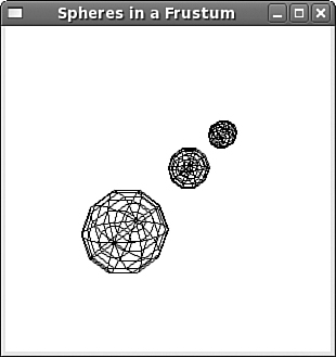
The glsphere application in the Chapter20 directory uses a perspective projection to display three spheres with the same radius. Because of its placement in the frustum, the sphere in front is much larger than the other two. This is shown in Figure 20.3.
The init function configures the window’s viewing region, and the code is presented here:
void init(void) {
   glClearColor(1.0, 1.0, 1.0, 0.0);
   glMatrixMode(GL_PROJECTION);
   glLoadIdentity();
   glFrustum(-2.0, 2.0, -2.0, 2.0, 2, 20.0);
   glMatrixMode(GL_MODELVIEW);
}
The first call to glMatrixMode tells the renderer that the following commands will affect the size/shape of the viewing region. glLoadIdentity sets the projection matrix equal to the identity matrix, and glFrustum updates the matrix so that all objects are displayed in a frustum whose near face is a 4x4 square and located at z = −2. The rear face is located at z = −20. The second call to glMatrixMode tells the renderer that further commands will affect either the objects in the region or the viewer’s line of sight.
Thus far, this chapter has covered the basics of creating a window with GLUT and defining the viewing region with OpenGL. The next step is more involved but also more interesting: building shapes to fit inside the viewing region.
OpenGL graphics are vertex oriented. That is, shapes are defined by creating points in space and setting characteristics for each point. OpenGL provides a number of characteristics that can be assigned to vertices, but this section focuses on two: colors and normal vectors. A vertex’s color determines how the point and its surrounding surface will be displayed. A vertex’s normal vector defines how the surrounding surface is aligned in space and determines how light should reflect from the surface.
Traditionally, vertex information is passed to the renderer one vertex at a time. However, it’s more efficient to group vertex characteristics together into a vertex buffer object, or VBO, and pass the entire VBO to the renderer. This section presents both methods.
In the preceding chapter, graphics were created by setting pixel values in the Linux frame buffer. Each point has two integer coordinates that correspond exactly to its position in the physical display. To create an actual shape, each pixel in the shape has to be individually colored.
The process is completely different with OpenGL. OpenGL points, called vertices, can be positioned in two or three dimensions using integer or floating-point coordinates. A point’s position places it in the viewing region, not the frame buffer. And with OpenGL, you only have to identify boundary points of a shape. Then you can tell OpenGL to fill the shape with color, display only the lines that connect points, or display the boundary points alone.
The functions glVertex2*, glVertex3*, and glVertex4* define individual vertices. The number in the function name determines how many values are required in the argument. For example, glVertex3* requires three values to define a point in three dimensions. The following code uses glVertex3* to create four vertices whose coordinate values have type glShort:
glVertex3s( 1,  1,  1);
glVertex3s(-1,  1,  1);
glVertex3s(-1, -1,  1);
glVertex3s( 1, -1,  1);
In OpenGL code, vertex definitions must be placed between calls to glBegin and glEnd. The argument of glBegin determines how the vertices are connected together and grouped into shapes. That is, it defines whether the vertices should be drawn as points in a line, triangle, quadrilateral, or polygon. Table 20.4 lists the possible values for the glBegin argument.
Table 20.4. Arguments of glBegin
Function Name | Description |
|---|---|
| Vertices drawn as unconnected points. |
| Each pair of vertices is drawn as a separate line. |
| Successive vertices are drawn as further points in a single line. |
| Like |
| Each triple of vertices is drawn as a triangle. |
| First three vertices define a triangle; each successive point defines a triangle connected to preceding two points. |
| First three vertices define a triangle; each successive point defines a triangle connected to first point. |
| Each group of four points is drawn as a quadrilateral. |
| First four vertices define a quadrilateral; each successive pair of points defines a quadrilateral connected to preceding two points. |
| Draws points as a single polygon. |
These constants are important and the best way to understand them is to see how they determine the shape of actual graphics. The following code creates two triangles from six points:
glBegin(GL_TRIANGLES);

   /* Triangle 1 */
   glVertex2s(1, 1);    /* v0 */
   glVertex2s(1, 4);    /* v1 */
   glVertex2s(3, 1);    /* v2 */

   /* Triangle 2 */
   glVertex2s(3, 3);    /* v3 */
   glVertex2s(3, 6);    /* v4 */
   glVertex2s(5, 3);    /* v5 */
glEnd();
Figure 20.4 shows how these six points are drawn for glBegin arguments of GL_LINES, GL_LINE_STRIP, GL_TRIANGLES, and GL_POLYGON.
The glBegin argument determines how shapes are formed from vertices and the function glPolygonMode provides additional information about how the shapes should be drawn. Its signature is given as follows:
void glPolygonMode(GLenum face, GLenum mode);
Here, mode specifies how shapes should be drawn, and face determines which shapes are affected. The mode argument can take one of three values:
GL_POINT: Only the vertices of the shape are drawn.GL_LINE: Only the boundary lines of the shape are drawn.GL_FILL: The boundary and interior of the shape are colored with the active color.
The face parameter can also take one of three arguments:
GL_FRONT: Only shapes facing the front of the viewing region are configured.GL_BACK: Only shapes facing the back of the viewing region are configured.GL_FRONT_AND_BACK: All shapes are configured byglPolygonMode.
To create the images in Figure 20.4, the polygon mode was defined with the following:
glPolygonMode(GL_FRONT_AND_BACK, GL_LINE);
This ensures that only the shapes’ boundary lines would be rendered.
In the glsphere code, the display function sets the color once for the entire application. This is done with the following command:
glColor3f(0, 0, 0);
The arguments identify the amount of red, green, and blue in the active color. Their datatype is GLclampf, which means their floating-point values are held between 0.0 and 1.0. When this function is called in ppu_glsphere.c, all following vertices are colored black.
Vertices can be colored individually by calling glColor3f before each vertex definition. For example, the points (1.0, 1.0, 1.0), (−1.0, 1.0, 1.0), (−1.0, −1.0, 1.0), and (1.0, −1.0, 1.0) can be colored red, green, blue, and gray with the following code:
glColor3f(1.0, 0.0, 0.0);    /* red */
glVertex3f(1.0, 1.0, 1.0);

glColor3f(0.0, 1.0, 0.0);    /* green */
glVertex3f(-1.0, 1.0, 1.0,);

glColor3f(0.0, 0.0, 1.0);    /* blue */
glVertex3f(-1.0, -1.0, 1.0);

glColor3f(0.25, 0.25, 0.25); /* gray */
glVertex3f(1.0, -1.0, 1.0);
In addition to glColor3f, there are glColor3* variants that accept integer (byte, short, int) arguments. These values are mapped to floating-point values such that the integer maximum corresponds to 1.0, and the minimum corresponds to 0.0. For example, glColor3ub(255, 255, 255) makes white the active color because 255 is the largest value an unsigned byte can take.
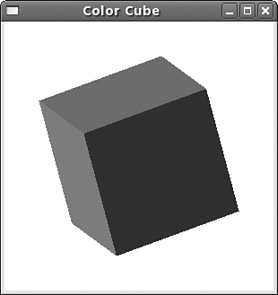
The Chapter20/glcube project creates a multicolored cube in three dimensions. Most of the code is similar to that in the glsphere project, but the display function calls glColor3f six times to color each face of the cube. Each call to glColor3f is followed by four calls to glVertex3sv, which sets the coordinates of the face’s vertices. The following code shows the content of the display function in ppu_glcube.c:
void display(void) {
   int i;

   /* Clear the window */
   glClear(GL_COLOR_BUFFER_BIT | GL_DEPTH_BUFFER_BIT);
   glLoadIdentity();

   /* Position cube in the region and rotate */
   glTranslatef(0, 0, -7);
   glRotatef(30, 1, 1, 1);

   glBegin(GL_QUADS);

      /* Color the top face red */
      glColor3f(1, 0, 0);
      glVertex3sv(topFace[0]);
      glVertex3sv(topFace[1]);
      glVertex3sv(topFace[2]);
      glVertex3sv(topFace[3]);

      /* Color the bottom face green */
      glColor3f(0, 1, 0);
      glVertex3sv(bottomFace[0]);
      glVertex3sv(bottomFace[1]);
      glVertex3sv(bottomFace[2]);
      glVertex3sv(bottomFace[3]);

      /* Color the front face blue */
      glColor3f(0, 0, 1);
      glVertex3sv(frontFace[0]);
      glVertex3sv(frontFace[1]);
      glVertex3sv(frontFace[2]);
      glVertex3sv(frontFace[3]);

      /* Color the back face yellow */
      glColor3f(1, 1, 0);
      glVertex3sv(backFace[0]);
      glVertex3sv(backFace[1]);
      glVertex3sv(backFace[2]);
      glVertex3sv(backFace[3]);

      /* Color the left face fuchsia */
      glColor3f(1, 0, 1);
      glVertex3sv(leftFace[0]);
      glVertex3sv(leftFace[1]);
      glVertex3sv(leftFace[2]);
      glVertex3sv(leftFace[3]);

      /* Color the right face aqua */
      glColor3f(0, 1, 1);
      glVertex3sv(rightFace[0]);
      glVertex3sv(rightFace[1]);
      glVertex3sv(rightFace[2]);
      glVertex3sv(rightFace[3]);

   glEnd();
   glutSwapBuffers();
}
Figure 20.5 shows the graphical result of this code converted into grayscale.
The display function defines vertices with glVertex3sv instead of the simpler variant, glVertex3s. The v at the end of the function specifies that the function accepts a pointer to an array of values rather than the values themselves. The v stands for vector, and can be attached to glColor* as well as glNormal*, the function discussed next.
Creating a three-dimensional object in OpenGL requires more than vertex placement and color. Unless the shape is a simple cube or pyramid, the contour of the surface has to be defined. In OpenGL, this information is provided in the form of normal vectors. A normal vector to a surface is the vector perpendicular to the surface—the vector that points out of the surface at the location of a given vertex.
Normal vectors in OpenGL are identified with the glNormal* function. This has five primary variants: glNormal3b, glNormal3s, glNormal3f, glNormal3i, and glNormal3d. Each of these defines a normal vector with three values. If glNormal* is followed by v, the argument is a pointer to an array of three values.
Normal vectors are assigned to vertices in the same way that colors are: When glNormal* is invoked, the normal vector applies to all vertices created with subsequent glVertex* calls. For example, the following code assigns a normal vector pointing in the x-direction to each vertex in a quadrilateral:
glBegin(GL_QUADS);
   glNormal3d(1, 0, 0);
   glVertex3fv(point1);
   glVertex3fv(point2);
   glVertex3fv(point3);
   glVertex3fv(point4);
glEnd();
The primary use of normal vectors is to define how light reflects from surfaces. The topic of OpenGL lighting and materials is fascinating but beyond the scope of this book.
An OpenGL graphic may contain thousands of vertices, so it’s important to transfer vertex data from the client (the OpenGL application) to the renderer (the GPU, remote system, or local application) as quickly and as efficiently as possible. Legacy applications send data for one vertex at a time, but modern applications transfer data in bulk. This is accomplished through memory mapping: Applications map a region of renderer memory into client memory, and then deliver graphic data in large blocks.
This block is composed of the same vertex information that has been described so far: coordinates, colors, and normal vectors. But the data is placed inside arrays that are combined into a vertex buffer object, or VBO.
VBOs make efficient use of channel bandwidth and are particularly efficient for applications where vertex data remains unchanged from frame to frame. If the VBO must be updated frequently, hints can be provided that identify how frequently the data will be accessed. Then the renderer can take whatever steps it needs to provide accessibility.
Making use of vertex buffer objects in code requires seven tasks:
Obtain a descriptor for the VBO.
Make the VBO the active array object.
Enable arrays to be sent to the renderer.
Allocate memory for the VBO and load data arrays.
Set pointers to the different data arrays in the VBO.
Draw the arrays using the VBO.
Deallocate the buffer after completion.
Table 20.5 lists the OpenGL functions associated with vertex buffer objects. The leftmost column identifies which task associated with the function.
Table 20.5. OpenGL Functions for VBOs and Arrays
Task | Function Name | Install |
|---|---|---|
1 |
| Create |
2 |
| Makes the buffer object identified by |
3 |
| Enable client ability to create the array identified by |
4 |
| Allocates memory for the buffer object and identifies the data that should be loaded into the buffer |
4 |
| Identifies data to be placed in a portion of the buffer |
5 |
| Identify size, datatype, and placement of vertex data in array |
5 |
| Identify size, datatype, and placement of color data in array |
5 |
| Identify datatype and placement of normal data in array |
6 |
| Starting from |
7 |
| Delete |
The glGenBuffers function produces an array of VBO descriptors. To make a buffer object active, its descriptor must be matched to a target with glBindBuffer. If the VBO will store data from an unindexed array, the target GL_ARRAY_BUFFER should be used. The array must be enabled on the client with glEnableClientState(state). Common values for state include GL_VERTEX_ARRAY, GL_COLOR_ARRAY, and GL_NORMAL_ARRAY.
glBufferData sets aside memory for the buffer object and loads array data into the allocated memory. glBufferSubData loads data into a portion of an existing VBO. In both cases, the first argument is the target identified in glBindBuffer. Both functions require the size of the data to be loaded and a pointer to the data itself. An important difference between them is that glBufferData accepts a usage value that tells the renderer how the buffered data will be accessed.
There are nine possible values for the usage parameter. They’re divided into three categories depending on how frequently the VBO will be accessed:
If the VBO will be changed once and only accessed a few times, use one of the
STREAMconstants:GL_STREAM_READ,GL_STREAM_DRAW, andGL_STREAM_COPY.If the VBO will be changed once and accessed many times, use one of the
STATICconstants:GL_STATIC_READ,GL_STATIC_DRAW, andGL_STATIC_COPY.If the VBO will be changed and accessed many times, use one of the
DYNAMICconstants:GL_DYNAMIC_READ,GL_DYNAMIC_DRAW, andGL_DYNAMIC_COPY.
The DRAW constants specify that the data will be written to by the application and used for drawing. The READ constants specify that the data will be read by the application, and the COPY constants specify that the data will be read from, written to, and used for drawing.
As an example, the vertex_data and color_data arrays contain 20 elements each. The following code generates a VBO descriptor, vbo_desc, binds it to the target, and loads the arrays into the buffer object:
GLuint vbo_desc;

/* Generate a single VBO descriptor */
glGenBuffers(1, &vbo_desc);

/* Bind the descriptor to the target */
glBindBuffer(GL_ARRAY_BUFFER, vbo_desc);

/* Enable vertex and color arrays on the client */
glEnableClientState(GL_VERTEX_ARRAY);
glEnableClientState(GL_COLOR_ARRAY);

/* Load vertex_data and color_data into the VBO */
glBufferData(GL_ARRAY_BUFFER, 40*sizeof(GLfloat),
   vertex_data, GL_STREAM_DRAW);

glBufferSubData(GL_ARRAY_BUFFER, 20*sizeof(GLfloat),
   20*sizeof(GLfloat), color_data);
Before the renderer can use the VBO, it needs to know the locations of the VBO’s arrays and the nature of the data contained in the arrays. This information is supplied with the gl*Pointer functions, which include glVertexPointer, glColorPointer, and glNormalPointer. Each of these functions identifies the size and datatype of the corresponding array, as well as its location in the VBO and the stride between elements.
The vertices in the VBO are rendered with glDrawArrays. Its first argument, mode, is like the argument of glBegin, and identifies how the vertices are grouped into shapes. The second argument identifies the index of the first vertex to be drawn. The last parameter is the total number of vertices to be rendered. glDeleteBuffers uses a descriptor to deallocate the corresponding buffer object, and removes the object’s binding to the target.
OpenGL coding is an interesting but involved topic. Its API is vast, has multiple implementations, and is currently undergoing tremendous changes. To use it effectively, you need to have a solid understanding of geometry, matrices, and vectors. Despite the steep learning curve, however, if you’re going to build three-dimensional graphics in Linux, there’s no better library available.
This chapter began with an introduction to OpenGL’s past and present. The open source implementation of OpenGL is called Mesa, which is being reworked into a new architecture called Gallium. The Gallium driver for the Cell is still in an early stage of development, but it can be downloaded with Mesa and used to build the shared libraries required for OpenGL.
The OpenGL Utility Toolkit, or GLUT, provides the binding that makes it possible to run OpenGL applications inside the windows of an operating system. Inside a GLUT window, a viewing region is the space that holds OpenGL graphics. This region can be two dimensional or three dimensional, and can provide an orthographic projection (all objects right sized) or a perspective projection (objects appear smaller at distance).
OpenGL shapes are composed of vertices that identify points in the viewing region. Colors can be assigned to each vertex, and a normal vector is used to tell which direction is perpendicular to the vertex’s surface. For the sake of efficiency, this vertex data can be packaged in a vertex buffer object (VBO) and sent from the client to the renderer.
This shamefully brief treatment has barely scratched the surface of OpenGL’s powerful API. Topics such as textures, shaders, and animation have been left by the wayside, but this material should provide a firm foundation from which to continue your study. The subject of the next chapter, Ogre3D, builds on OpenGL’s graphics capabilities to create games.