
The PowerPC Processor Unit (PPU) has many strengths, but the Cell’s extraordinary computing capability comes from its Synergistic Processor Units (SPUs). Unlike the general-purpose PPU, the SPUs were designed with a single goal in mind: high-speed vector processing. You won’t use SPUs for text processing, code compiling, or e-mail; but if you need to transform hundreds of thousands of pixels to a new coordinate system, SPUs will get the job done quickly.
The SPU’s architecture is much simpler than the PPU’s. There are no caches, no threads, no paging, and no memory segments. There are only two types of user registers. With the SPU, you don’t have to worry about microcoded instructions, cache hits or hints, virtual memory, or which resources are duplicated between threads.
But when you write SPU applications, there’s a greater need to keep track of low-level details. An SPU can access only 256KB of memory, so it’s critical to monitor the size of the executable, stack, and heap. In many applications, the limited storage makes it necessary to transfer data to and from main memory with direct memory access (DMA). So despite the SPU’s architectural simplicity, coding applications still presents a wealth of challenges that all dedicated programmers will be sure to enjoy.
This chapter doesn’t discuss DMA or interprocessor communication. Instead, it starts with a brief overview of the SPU’s structure and then covers the SPU’s available datatypes and function libraries. The local store (LS) is examined in depth, and the chapter ends with a discussion about the SPU’s call stack and heap.
The mission of the SPU is simple. It pulls 128-bit vectors from the LS into its register file, processes instructions that access the registers, and stores the output vectors to the LS. This simplicity of purpose is reflected in its functional units and register file.
Figure 10.1 shows the processing elements that make up the SPU. Instructions flow from the SPU Control Unit (SCN) to other functional units depending on the nature of the instruction to be processed. Data flows into the SPU’s registers through the SPU Load/Store Unit (SLS) and then travels back to the LS.
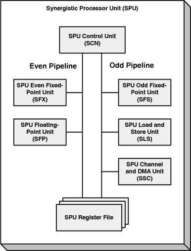
There are three important differences between the SPU’s structure and the PPU’s structure, shown in Figure 6.3:
No cache or effective/virtual memory: The only memory an SPU can directly access is its LS and register file.
No scalar units: Every SPU unit operates on 128-bit vectors.
Two distinct pipelines: An SPU instruction can take one of two paths (odd or even) as it travels from the SCN to its execution unit.
This last point is important to understand. Generally speaking, the units connected to the even pipeline perform mathematical operations, and the units on the odd pipeline handle everything else. The advantage of having two pipelines is that their corresponding units operate in parallel. For example, an SPU can read and write from memory and perform high-speed vector math at the same time.
The functions of these units are as follows:
SPU Control Unit (SCN)—. Fetches and dispatches instructions to the execution units and performs branching and all other control operations
SPU Even Fixed-Point Unit (SFX)—. Handles arithmetic/logic operations and performs comparisons and reciprocation on floating-point values
SPU Odd Fixed-Point Unit (SFS)—. Shifts quadwords; rotates words, halfwords, bytes, and bits; and shuffles bytes
SPU Floating-Point Unit (SFP)—. Performs operations on single-precision and double-precision floating-point values, multiplies and converts integers
SPU Load/Store Unit (SLS)—. Performs loads and stores, manages the branch target buffer (BTB), and sends DMA requests to the LS
SPU Channel and DMA Unit (SSC)—. Communicates with the Memory Flow Controller (MFC) and controls DMA data transfer
The SCN can fetch 32 instructions at a time. Chapter 11, “SIMD Programming on the SPU,” describes vector processing with the SFP, SFX, and SFP. Chapter 12, “SPU Communication, Part 1: Direct Memory Access (DMA),” explains the SSC and the MFC.
The SPU’s functional units operate on values stored in the SPU’s register file. Unlike the PPU, which has a wide array of registers with different sizes and functions, the SPU has only two types of user registers: the general purpose registers (GPRs) and the floating-point status and control register (FPSCR). Both are 128 bits in size and are shown in Figure 10.2.
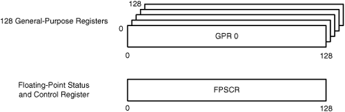
The GPRs store all the information—data and instructions—used by the functional units. Altogether, they provide 16KB of storage and serve as both the SPU’s instruction cache and data cache. Each read or write to the SPU register file requires two cycles.
The FPSCR stores information related to the results of floating-point operations, such as whether an operation returned a denormalized value or attempted to divide by zero. Accessing this register is important to gain information about processing errors and special conditions. Chapter 11 discusses the FPSCR in detail.
The SPU’s datatypes (scalar and vector) are similar to the PPU’s, but new types are available for processing 64-bit values. The SPU processes floating-point values in much the same way as the PPU, but there are differences regarding which values and errors it accepts.
Table 10.1 lists the scalar datatypes supported by the SPU. Like the PPU, the bits are arranged in big-endian order: the most significant bit (MSB) is on the far left and the least significant bit (LSB) is on the far right.
Table 10.1. SPU Scalar Datatypes
Datatype Name | Content | Size |
|---|---|---|
| True/False | 1 byte |
| ASCII character/integer (−128 to 127) | 1 byte |
| Integer (0 to 255) | 1 byte |
| Short integer (−32,768 to 32,767) | 2 bytes |
| Short integer (0 to 65,535) | 2 bytes |
| Integer (−2,147,483,648 to 2,147,483,647) | 4 bytes |
| Integer (0 to 4,294,967,295) | 4 bytes |
| Single-precision floating-point value | 4 bytes |
| Double-precision floating-point value | 8 bytes |
| Integer (−9,223,372,036,854,775,808 to 9,223,372,036,854,775,807) | 8 bytes |
| Integer (0 to 18,446,744,073,709,551,615) | 8 bytes |
| Instruction-dependent | 16 bytes |
There are two differences between the SPU datatypes in Table 10.1 and the PPU datatypes in Table 6.1. First, there is no w_char datatype representing wide characters. Second, the last datatype in the table, qword, is available only on the SPU. qwords are required as arguments for a set of SPU functions called specific intrinsics.
As mentioned earlier, the SPU’s GPRs are 128 bits wide. When a scalar is stored in a register, it’s placed in its preferred slot. For example, if var is a halfword stored in the register, it will occupy Bytes 2 and 3 of the register. These bytes form the halfword’s preferred slot. When another operation needs to access var, it will only access these bytes of the register. Figure 10.3 shows how other scalars are stored in the SPU’s registers.
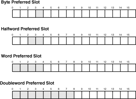
As shown, using a 16-byte register to store a byte or halfword is a terrible waste of memory. Whenever possible, combine scalars within a vector and perform operations on the vector instead.
Table 10.2 lists the different types of vectors supported by the SPU. AltiVec’s vector pixel type is gone along with the vector bool datatypes. The three new vector types are shown in boldface.
Table 10.2. SPU Vector Datatypes
Vector Datatype | Scalar Elements |
|---|---|
| 16 8-bit unsigned chars |
| 16 8-bit signed chars |
| 8 16-bit unsigned shorts |
| 8 16-bit signed shorts |
| 8 16-bit unsigned halfwords |
| 4 32-bit unsigned ints |
| 4 32-bit signed ints |
| 4 32-bit floats |
| 2 64-bit unsigned long longs |
| 2 64-bit signed long longs |
| 2 64-bit doubles |
These last three vector datatypes store 64-bit scalars, and the ability to process vectors of 64-bit elements is one of the SPU’s advantages over the PPU. The vector unsigned long long and vector signed long long datatypes are straightforward to understand, but the way the SPU processes floating-point values inside vector floats and vector doubles requires further explanation.
If you’re porting an application to run on the SPU, it’s important to know how it processes floating-point values. Specifically, you need to know to what extent the SPU adheres to the common IEEE-754 standard. Figure 10.4 shows how the PPU and the SPU store floating-point values, and this format fully complies with the standard.
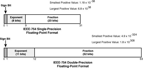
When it comes to processing these values in applications, however, the PPU and SPU deviate from the standard in different ways. Section 9.1, “From Scalars to Vectors,” discusses how the PPU processes floating-point vectors and its different operational modes. The SPU supports only one mode of operation, although it treats single-precision and double-precision values differently.
In processing single-precision values, the SPU differs from the standard in the following respects:
All denormalized numbers are forced to zero.
If an exponent is all 1s, the number is treated as a normal number rather than as
inforNaN.There are no Round to Nearest, Round to +Infinity, or Round to −Infinity rounding modes; only Round to Zero is supported.
In processing double-precision values, the SPU supports NaNs and all rounding modes. It responds to denormalized values by forcing them to zero and raising a bit in the FPSCR. It also sets bits in the FPSCR in the events of overflow, underflow, inexact result, invalid operation, and NaN value propagation. These errors and the FPSCR are fully described in Chapter 11.
The SPU multipliers in the first-generation Cell only operate on 16-bit operands. For this reason, 32x32-bit integer multiplies require five instructions: three multiplications and two additions. For the sake of efficiency, use shorts as often as possible and make sure to cast constants (usually processed as ints) and small values as unsigned shorts.
The SPU is a resource-limited, special-purpose processor, and its function libraries are similarly limited and specialized. Many of the header files in the C and C++ standard libraries header files are available for the SPU, but functions requiring an operating system or file system generally don’t run properly.
Most of the elements in the C standard library and the C++ standard library are available for the SPU. Table 10.3 lists the header files in both categories.
Table 10.3. C/C++ Standard Library Elements
Available C Headers | Available C++ Headers | Unavailable C Headers | Unavailable C++ Headers |
|---|---|---|---|
|
|
|
|
|
|
|
|
|
|
|
|
|
|
|
|
|
|
|
|
|
|
| |
|
|
| |
|
|
| |
|
|
| |
|
|
| |
|
|
| |
|
|
| |
|
|
| |
|
|
| |
|
| ||
|
| ||
[*] |
| ||
[*] |
| ||
[*] |
| ||
| |||
[*] This header file is provided, but certain functions/types are unavailable. See following discussion. | |||
The three starred headers in the first column can be included in SPU code, but the following functions and types are missing:
stddef.h:Thewchar_ttype is unavailable (no wide characters on the SPU).stddef.h:Missinggetenv(),mblen(),mbstowcs(),system(),wcstombs(), andwctomb().stdio.h:Onlyprintf()is available.
This last bullet demands further explanation. printf() can be called in SPU code, but the SPU calls on the PPU to send the text to standard output. This is called an externally assisted function call, and because of the time required to execute, printf() should be used only when timing isn’t critical.
The Cell SDK includes a number of helpful routines beyond those in the C/C++ standard libraries, and those declared in spu_intrinsics.h are foremost among them. These functions provide low-level access to the SPU instruction set. The main difference between SPU and PPU intrinsics is that SPU intrinsics start with spu_, and PPU intrinsics start with two underscores.
The SPU has no Time Base register, so there are no SPU intrinsics that perform the same function as the PPU’s __mftb(). However, the SPU has a decrementer that counts ticks within an application. This is discussed in Chapter 11.
Most of the functions in spu_intrinsics.h operate on vectors. These aren’t the same as the PPU functions in altivec.h, but they cover the same territory. Because vector processing is so important for SPU coding, Chapter 11 describes them in detail. The Cell SDK also provides the SIMD Math library and the MASSV library, which provide high-level floating-point routines for vector mathematics.
In addition to vector functions, the spu_intrinsics.h header declares functions called specific intrinsics, which map immediately to assembly language commands. Their names are similar to SPU assembly instructions, but each function starts with si_. For example, the specific intrinsic si_stqa(a, addr) stores the qword a into memory at addr, and this performs exactly the same operation as the assembly command stqa a addr. Chapter 15, “SPU Assembly Language,” discusses SPU assembly language and SPU specific intrinsics.
The Cell SDK provides many SPU libraries whose functions perform advanced mathematics and signal processing. The routines in libfft perform fast Fourier transforms (FFTs), the functions in libmc_rand generate and operate on random values, and the functions in liblarge_matrix operate on large matrices. There are also libraries for multiprecision mathematics, image manipulation, curves, and surfaces. This book doesn’t explain all the available functions, but the following chapters cover quite a few.
Besides the register file, the local store (LS) is the only memory that the SPU can access directly. It can be updated through DMA requests, but it’s not cache; the LS is just SRAM and can be read or written to only once per cycle.
There are three types of operations that access the LS:
DMA (high priority): Transfers data in blocks of 1, 2, 4, 8, or 16 bytes, and in multiples of 16 bytes up to a maximum of 128 bytes
SPU load/store (medium priority): Reads or writes one 16-byte line at a time
Instruction fetch (low priority): Reads eight lines (128 bytes) of the LS at once
The LS stores 256KB of memory, which means it can hold only 2,048 lines of instructions and data. This is shown in Figure 10.5. The LS is byte addressed, but because it must be accessed in 16-byte blocks, the last 4 bits of the address are ignored for most memory operations.
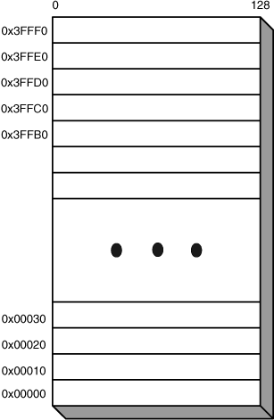
There are no effective addresses or virtual addresses in the SPU; all the addresses used in applications are real addresses. If you display the address of a vector in an application, the result (between 0 and 0x3FFF0) represents the vector’s actual location in the LS.
The SPU linker (spu-ld) provides an option that displays how the LS will be apportioned for an application. It creates a file that lists the sections and symbols contained in the SPU executable [1] and the LS addresses the linker assigned them to. This is called a map file, and contains a great deal of information.
To tell the linker to create a map file, insert the following flag into the build command:
-W,-Map=filename
For example, the following command tells the linker to create a map file called map.txt during the creation of app:
spu-gcc -o app app.c -W,-Map=map.txt
The small memory space presents another reason to think of data in terms of vectors rather than scalars. The SPU loads and stores data in 16-byte blocks only, so a scalar will take up as much space as a vector. It’s hard to avoid scalars altogether, but the more you combine data into vectors, the faster your code will run and the more space you’ll have available.
In addition to local reads, writes, and instruction fetches, the LS can be accessed by the PPU and other SPUs. This external access becomes a concern when a local SPU executable requires commands to execute in specific order. The SPU guarantees that local loads and stores will be executed in program order, but instruction fetches and external operations may take place at any time. This method of distributed memory access is referred to as weakly consistent.
In circumstances where the SPU’s memory access must be performed in a particular order relative to external instructions, spu_intrinsics.h declares three useful functions:
spu_dsync():Forces loads, stores, and external accesses to complete before continuingspu_sync():Forces loads, stores, external accesses, and instruction fetches to complete before continuingspu_sync_c():Forces loads, stores, external accesses, instruction fetches, and channel writes to complete before continuing
These functions, listed in order of increasing severity, effectively halt the SPU’s instruction processing until the right conditions are met. This can significantly degrade the SPU’s performance.
Chapter 7, “The SPE Runtime Management Library (libspe),” described the process of managing SPU execution in PPU code: Create a program handle from the SPU executable, load the program handle into the SPU context, and run the SPU context. This section looks closer into what’s happening on the SPU and focuses on how the PPU initializes the SPU’s data. The SPU stack plays an important role in this discussion.
After the PPU selects an SPU to run the executable, it initializes the contents of the SPU’s registers and LS. For example, Chapter 7 explained that the SPU can receive three values in its main function: speid, argp, and envp. These are placed in Registers 3, 4, and 5, respectively. The CBE Linux Application Binary Interface (ABI) specifies how initialization information is placed in SPU registers, and its guidelines are listed in Table 10.4.
Table 10.4. SPU Register Usage
Register | Name | Datatype | Function |
|---|---|---|---|
R0 | LR |
| Stores the function’s return address |
R1 | SP |
| Pointer to the top of the initial stack |
R2 | SS |
| Size of the stack |
R3 | speid |
| Identifies the SPU thread for the PPU |
R4 | argp |
| Pointer to array of SPU parameters |
R5 | envp |
| Pointer to environment structure |
R6 to R74 | — | — | Stores additional function parameters |
R75 to R79 | — | — | Scratch registers |
R80 to R128 | — | — | Holds local variables |
The call stack is the portion of LS that stores information about currently executing SPU functions. When a function is called, its return address, parameters, and local variables are stored at the memory address contained in R1. This address, called the stack pointer, is then decremented to point to the next free section of memory. When the function completes, the stack pointer returns to its earlier value.
To maximize the amount of available stack space, the PPU initializes the SPU’s stack pointer to the topmost line in the SPU’s LS (0x3FFF0). The next line, 0x3FFE0, is set aside for the return address of the next function. Figure 10.6 (left side) shows what this initial state looks like.
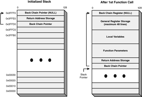
With each new function call, the stack grows downward to accommodate its parameters, local variables, and necessary registers. This is shown in Figure 10.6 (right side). The SP is decremented to contain the address at the bottom of the stack. The LS memory at that address, called the back chain pointer, stores the address of the previous SP.
The code in Listing 10.1 gives a clearer idea of how the stack works. The main function calls foo, bar, and baz, and displays the stack pointer (R1) after each call.
Example 10.1. Displaying the SPU Stack Pointer: spu_stacktest.c
#include <stdio.h>

/* Set stack_ptr equal to Register 1 */
register volatile unsigned int *stack_ptr asm("1");

int foo(int);
int bar(int);
int baz(int);

/* foo calls bar */
int foo(int fooval) {
   printf("Foo Stack Ptr: %p
", stack_ptr);
   return bar(2*fooval);
}

/* bar calls baz */
int bar(int barval) {
   printf("Bar Stack Ptr: %p
", stack_ptr);
   return baz(2*barval);
}

/* baz returns twice the input */
int baz(int bazval) {
   printf("Baz Stack Ptr: %p
", stack_ptr);
   return 2*bazval;
}

/* main calls foo */
int main(int argc, char **argv) {
   printf("Main Stack Ptr: %p
", stack_ptr);
   return foo(2);
}
On my system, the results are as follows:
Main Stack Ptr: 0x3ff90
Foo Stack Ptr: 0x3ff60
Bar Stack Ptr: 0x3ff30
Baz Stack Ptr: 0x3ff00
The stack decrements with each function call, but the stack pointer doesn’t drop significantly. This is because foo, bar, and baz have few parameters and no local variables. But remember: The more nontrivial nested functions you have in your code, the larger your stack will be and the more likely it is that the stack will overwrite critical memory space.
After the SPU is initialized, the load process is performed in three steps:
The PPU copies the SPU loader (spu_ld.so) into the last 512 bytes of the SPU’s LS.
The SPU loader copies the SPU executable into the LS.
The PPU places the loader’s entry point into the SPU’s program counter, and the SPU executable starts running.
Dynamic libraries required by an SPU executable are loaded into the LS before the executable starts. This is different from traditional dynamic loading, in which the library is loaded during execution.
Even though you can run SPU executables from the command line, you’re not accessing the SPU directly. Every call to an SPU executable is processed by the operating system running on the PPU. The PPU loads the executable onto an SPU and manages its operation in the manner described in Chapter 7.
In earlier versions of the SDK, SPU executables couldn’t be run on the command line and had to be executed with the elfspe command. Because they weren’t proper executables, they were called spulets. As of SDK 3.0, however, there’s no difference in usage between PPU and SPU executables, so no distinction will be made between them.
The stack allocates fixed amounts of memory for local variables, but in many cases, you might not know how much memory you need before an application starts. The SPU provides for dynamic memory allocation, and the region from which this memory is allocated is called the heap. Whereas the stack starts at the top of the LS and grows downward, the heap starts at the bottom and grows upward.
Memory alignment is an important concern when interfacing the LS, and the SDK provides specific functions that dynamically allocate and deallocate aligned memory. These functions are part of the Miscellaneous library, or libmisc. This library is provided for both the PPU and SPU, and can be found at $CELL_SDK/usr/lib or $CELL_SDK/usr/lib/spu.
Table 10.5 lists the memory allocation/deallocation functions provided by the Miscellaneous library.
Table 10.5. Dynamic Allocation Functions
Function Name | Purpose |
|---|---|
| Allocates size bytes at the given alignment |
| Allocates n*size bytes at the given alignment |
| Reallocates memory for ptr at the given size and alignment |
| Deallocates the memory pointed to by ptr |
| Returns the quadword at the unaligned address |
| Stores the quadword to the unaligned address |
The first four functions are similar to the common C allocation routines, but they accept an extra parameter that identifies the pointer’s byte alignment. This align parameter is an unsigned int that represents the base-2 logarithm of the alignment boundary. For example, to allocate 4096 bytes on a 128-byte boundary, you’d use
malloc_align(4096, 7)
because 2 7 = 128. Alignment is similar for calloc_align and realloc_align.
Note
Don’t confuse libmisc alignment with GCC’s aligned attribute. The first accepts the base-2 logarithm of the byte-alignment boundary (7 = 128-byte boundary), and the second accepts the actual number of bytes (128 = 128-byte boundary).
The last two functions in Table 10.5 make it possible to access the LS at unaligned memory locations. These functions only access 16-byte vectors: load_vec_aligned returns an unaligned vector, and store_vec_aligned stores an unaligned vector to memory.
It’s important to make sure that the stack and heap don’t overlap. This can happen when either the statically allocated or dynamically allocated memory takes up too much of the LS. The SPU doesn’t provide a heap pointer, but you can check the difference between the stack and heap by looking at the second element of Register 1. (The first element stores the stack pointer.) This is shown in Listing 10.2.
Example 10.2. Checking the Stack and Heap: spu_heaptest.c
#include <stdio.h>
#include <spu_intrinsics.h>
#include <libmisc.h>

/* Set reg_1 equal to Register 1 */
register volatile vector unsigned int reg_1 asm("1");

int main(int argc, char **argv) {

   /* Return stack-heap difference before allocation */
   printf("Before allocation: stack - heap = %#x
",
      spu_extract(reg_1, 1));

   /* Alloate 16K and display stack-heap difference */
   float* fl_array = malloc_align(0x4000, 7);
   printf("After allocation: stack - heap = %#x
",
      spu_extract(reg_1, 1));

   /* Deallocate memory */
   free_align(fl_array);
   return 0;
}
spu_extract is an SPU intrinsic function that retrieves a single element from a vector. The results on my system are as follows:
Before allocation: stack - heap = 0x3e5e0
After allocation: stack - heap = 0x3a350
The difference between the stack and heap decreases by nearly 16KB, which is the amount of memory allocated for fl_array.
The last and most involved topic of this chapter is the SPU’s instruction pipeline. This is the sequence of processing stages an instruction goes through from the time it’s fetched from the LS to the time it finishes executing. Like an assembly line, different stages process different instructions at once, and the more stages that are occupied, the faster the program will execute.
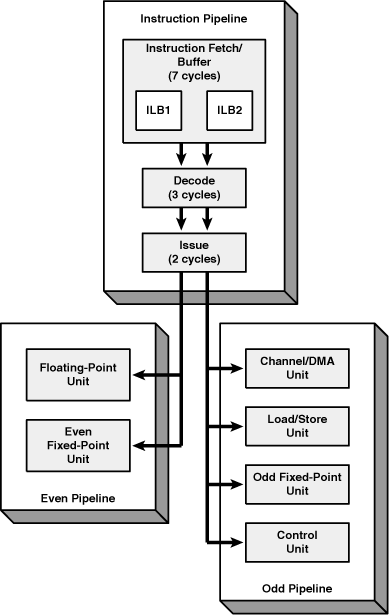
The SPU instruction pipeline is simpler than the PPU’s, but still relies on the same essential stages. First, the SPU Control Unit (SCN) takes instructions from memory before it needs them (prefetch) and stores them in one of two buffers. For each instruction, the SCN determines where the instruction should go (decode) and delivers it to its destination (issue). Figure 10.7 shows these stages.
To explain how the SPU pipeline operates, this section considers a hypothetical example in which the SCN is about to process the instructions shown in Figure 10.8. After assembly, each instruction takes up 4 bytes. This means that LS vectors (16 bytes each) contain four instructions.
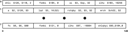
When the SPU starts running an executable, the SCN fills its instruction buffers (ILBs), which can each store 32 instructions. When one of the ILBs is empty, the SCN prefetches 32 more instructions to fill it. In this example, the SCN needs the 32 instructions shown in Figure 10.8.
The SPU has no way to cache instructions, so it always reads from the LS. Specifically, it sends a request to the SLS and asks for eight lines of instructions. After making the request, the SCN continues processing the instructions in its full buffer.
If there’s too much traffic between the SPU and its LS, the SCN may not get its instructions in time, and both instruction buffers will sit empty. When this happens, the SCN runs out of instructions to send into the pipeline. This condition is appropriately called runout. Runout temporarily halts your application, but you can prevent this condition by not performing load/store instructions in tight groups.
The SCN fetches instructions in two other situations. If the pipeline is purposefully emptied, or flushed, the SCN makes a new instruction request. This may occur because of spu_sync() or because the SCN incorrectly predicted a branch address. The second situation occurs when the SCN needs to fetch instructions because of an upcoming branch.
A branch instruction tells the SPU to stop fetching instructions in its current sequence and start processing instructions at a new address. There are two types of branch instructions:
Conditional—. The branch address depends on a comparison.
Unconditional—. The branch address is constant.
Conditional branches are more important because they force the processor to predict which of two addresses will be taken. The PPU, with its Branch History Tables (BHTs), uses a combination of dynamic and static methods to make its prediction. This is discussed in Section 6.3.
The SPU has no resources for dynamic prediction, and relies on static prediction alone. This assumes that each branch is part of a loop, such as a for or while..do loop. Further, it assumes that the loop will go backward. That is, it predicts that the comparison will return true and that the branch will go to the lesser of the two possible addresses. After making this prediction, the SCN fetches instructions at the predicted address and stores them in a hint target buffer (ILBH). When the actual branch instruction is processed, these instructions are inserted into the pipeline.
At some point, the loop is going to branch forward, and the SPU’s prediction will be mistaken. When the SCN detects this, it responds by flushing its pipeline and fetching new instructions. The penalty for a branch miss is 18 cycles, so it pays to do everything you can to avoid branches in your code. If your code is branch intensive, you might be better off running the routine on the PPU.
The SPU’s decode stage is similar to the PPU’s. This stage receives two instructions from the buffer every two cycles. It analyzes both instructions and determines which of the SPU’s functions units should receive the instructions.
For example, the first instruction in Figure 10.8 is shli $126, $110, 2. The shli command stands for Shift Left Word Immediate, and the instruction shifts the bits in Register 110 left twice and stores the result in Register 126. During the decode stage, the SCN determines that this instruction should be processed by the even-pipeline SPU Fixed Point Unit (SFX). Then it issues the instruction to this unit.
The decode stage also checks for dependency errors. These occur when instructions access memory or the register file out of proper order. For example, if one instruction attempts to read from a register before another instruction writes to it, a Read-After-Write (RAW) data hazard occurs. If the decode stage detects a hazard or error, the issue stage will stall until the instructions are properly reordered.
After decoding the pair of instructions, the SCN sends one or both of them to their appropriate execution units. Whether one or both of them issues depends on which pipeline (odd or even) the instructions are sent to. If the first instruction is issued to a unit on the even pipeline and the second is issued to the odd pipeline, both instructions can be issued in one cycle. Otherwise, the first instruction will be issued in the first cycle, and the second will be issued in the next cycle.
The example code in Figure 10.8 is taken from a compiled SPU application where the compiler has ensured that the instructions will issue two at a time. The first command, shli, is processed by the SPU Fixed-Point Unit on the even pipeline, and the second, fsmbi, is processed by the SPU Load/Store Unit on the odd pipeline. Therefore, the two of them will issue at the same time. In circumstances where this is impossible, you can insert nop (even pipeline) and lnop (odd pipeline) as placeholder instructions. Chapter 15 discusses these instructions and the rest of the SPU’s instruction set.
The SPU is a fascinating processor, and the goal of this chapter has been to describe what it’s made of and how it works. In making this description, I’ve tried to start as simply as possible, with registers and supported datatypes, and proceed to advanced topics. I hope this treatment is sufficient for both casual developers and obsessed coders seeking to make the most of every execution cycle.
The SPU’s structure reflects its no-frills approach to number crunching. The LS is as uncomplicated as memory gets: It’s not cache or cached, it makes no distinction between data and instructions, and it’s always accessed one 128-bit line at a time. When you look at the SPU’s functional units, you’ll see that their only purpose is to load lines from the LS, process them, and store them back to memory. This simplicity can cause problems when 256KB isn’t enough for your application, but as you’ll see, there are many ways to mitigate this concern.
You don’t have to remember every detail about the SPU’s executable loading and instruction pipeline, but you should keep two points in mind. First, always have a basic idea of what’s going on in the LS. This will prevent stack overruns and instruction runout. Second, try to keep your branches (if statements, switch/case statements, and so on) to a minimum. Mispredicted branches waste many cycles, and every branch requires a new instruction fetch that may turn out to be unnecessary.
This chapter has explained what makes the SPU unique, but you might not have a good idea as to what makes it so incredible. To appreciate the SPU in full, you need to understand the vector functions it can execute and how quickly it can execute them.
[1] For more information about ELF sections and symbols, read Appendix A, “Understanding ELF Files.”