
This chapter discusses two important SDK libraries whose capabilities can be used in many different applications. The first is the Multiprecision Math library, or libmpm, and the second is the Monte Carlo library, or libmc_rand. Both libraries provide functions that generate and manipulate special kinds of numbers.
The functions in the Multiprecision Math library operate on signed and unsigned integers that, by default, can occupy up to 4096 bits. Numbers of this size are important in cryptography, number theory, and any computation requiring values larger than 64-bit long longs. libmpm not only contains basic arithmetic functions for multiprecision numbers, but also advanced routines for operations such as modular reduction and modular exponentiation. These routines are crucial in data security, and the discussion of libmpm concludes with a full example of RSA encryption.
The Monte Carlo library, libmc_rand, provides functions that generate and transform sequences of numbers that resemble random numbers. Specifically, it generates number sequences using the Kirkpatrick-Stoll, Mersenne Twister, and Sobol methods. The distribution of these sequences can then be transformed using the Box-Muller algorithm, Moro’s inversion, or the Polar method.
In his fine book Cryptography in C and C++, Michael Welschenbach spends many chapters developing functions that operate on numbers comprising hundreds and thousands of bits. These functions are vital in Internet security and find application throughout computational mathematics. With libmpm, these routines are already available, and as a later example will show, they provide a solid foundation for implementing cryptographic methods such as RSA.
The multiprecision numbers we’ll be dealing with can be positive or negative, but they’re all integers. The functions in libmpm access these numbers as arrays of vector unsigned ints. For example, to allocate memory for a 512-bit integer called big_int, you’d create an array of 512/128 = 4 vectors, as shown here:
vector unsigned int big_int[4];
In this example, the pointer big_int would be passed into the libmpm functions and its size would be given as 4.
The maximum allowable size is determined by the MPM_MAX_SIZE parameter. This is set to 32, which means that multiprecision numbers can have up to 128 * 32 = 4096 bits. The bits of a multiprecision number are ordered in big-endian fashion, just as they are inside a vector.
This presentation of libmpm consists of two parts: general-purpose arithmetic/logic functions and multiprecision division/modular functions. The functions in the first category are easy to understand, but those in the second require additional explanation.
Table 18.1 lists the general-purpose routines in libmpm that operate on multiprecision values. In each entry, vec is short for vector unsigned int. The size parameter identifies how many vector unsigned ints make up the multiprecision value.
Table 18.1. General-Purpose Multiprecision Functions
Function Name | Purpose |
|---|---|
| Set |
| Set |
| Set |
| Set |
| Set |
| Perform a partial sum of two values. Accept |
| Set |
| Set |
| Set square equal to |
| Set |
| Set |
| Return all 1s if |
| Return all 1s if |
| Return all 1s if |
| Return all 1s if |
| Return all 1s if |
| Return all 1s if |
| Reverse the bit ordering of the contents of the multiprecision number in |
| Return index of highest non-0 quadword in |
None of these functions initialize a multiprecision value. The vectors in the value must be initialized individually.
The first two functions are concerned with the sign of the input multiprecision value. mpm_abs sets the input number equal to its magnitude and mpm_neg sets the number equal to its negation.
The usage of mpm_add, mpm_add2, and mpm_add3 depends on the size of the operands and the sum. mpm_add assumes that the operands and sum have the same size, and returns a vector containing the carry result. mpm_add2 assumes that the operands have different sizes and returns the size of the sum. mpm_add3 also assumes that the operands have different sizes, but accepts the size of the sum as a function argument.
mpm_add_partial is similar to mpm_add, but carry is a multiprecision value that serves as both input and output. This makes it possible to add multiple multiprecision values with a single carry value. For example, let’s say you want to add three 256-bit numbers. The same carry value is updated with each addition and is used at the end to augment the running sum. This is shown in Figure 18.1.
To implement this in code, mpm_add_partial must be called twice: once to add the first two inputs, and once to add the third input to the temporary sum. Then mpm_add adds the carry to the temporary sum. This is shown in Listing 18.1, which adds three vectors containing repeated 0xAAAAAAAA, 0xBBBBBBBB, and 0xCCCCCCCC sequences.
Example 18.1. Multiprecision Addition: spu_mpm_add.c
#include <stdio.h>
#include <libmpm.h>
#include <spu_intrinsics.h>

#define SIZE 2

int main() {

   int i, j;

   /* Create multiprecision values x, y, and z */
   vector unsigned int x[SIZE], y[SIZE], z[SIZE];

   /* Declare the carry, temp sum, and sum */
   vector unsigned int carry[SIZE], tmp_sum[SIZE],
      sum[SIZE+1];

   for (i=0; i<SIZE; i++) {
      x[i] = (vector unsigned int)
         {0xAAAAAAAA, 0xAAAAAAAA, 0xAAAAAAAA, 0xAAAAAAAA};
      y[i] = (vector unsigned int)
         {0xBBBBBBBB, 0xBBBBBBBB, 0xBBBBBBBB, 0xBBBBBBBB};
      z[i] = (vector unsigned int)
         {0xCCCCCCCC, 0xCCCCCCCC, 0xCCCCCCCC, 0xCCCCCCCC};
      carry[i] = (vector unsigned int)
         {0x00000000, 0x00000000, 0x00000000, 0x00000000};
      tmp_sum[i] = (vector unsigned int)
         {0x00000000, 0x00000000, 0x00000000, 0x00000000};
   }

   /* Perform the addition */
   mpm_add_partial(tmp_sum, x, y, carry, SIZE);
   mpm_add_partial(tmp_sum, z, tmp_sum, carry, SIZE);

   /* Set the first vector in sum */
   vector unsigned char sum_vec = {128, 128, 128, 128, 128,
      128, 128, 128, 128, 128, 128, 128, 28, 29, 30, 31};
   sum[0] = spu_shuffle(carry[0], carry[0], sum_vec);

   /* Shift the rest of the carry values into the sum */
   sum_vec = (vector unsigned char){4, 5, 6, 7,
      8, 9, 10, 11, 12, 13, 14, 15, 16, 17, 18, 19};
   for (i=1; i<SIZE; i++) {
      sum[i] = spu_shuffle(carry[i-1], carry[i], sum_vec);
   }

   /* Shift the last carry value */
   sum[SIZE] = spu_slqwbyte(carry[SIZE-1],
      sizeof(unsigned int));

   /* Add the sum to the tmp_sum */
   mpm_add2(sum, tmp_sum, SIZE, sum, SIZE+1);

   /* Display results */
   printf("Sum:
");
   for (i=0; i<SIZE+1; i++) {
      for (j=0; j<4; j++)
         printf("%08x ", spu_extract(sum[i], j));
      printf("
");
   }
   return 0;
}
The three multiplication functions, mpm_square, mpm_mul, and mpm_madd operate exactly as their names imply. The first multiplies a multiprecision value by itself, the second multiplies different numbers, and the third multiplies two numbers and adds a third. In each case, the quadword size of each input value must be identified.
The next six functions in the table compare multiprecision values. Like the similarly named SPU intrinsics, mpm_cmpgeq tests for equality, mpm_cmpgth tests for a greater-than relationship, and mpm_cmpgte tests for a greater-than-or-equal-to relationship. Each function has a second implementation that operates on values of different sizes. If a test succeeds, the function returns an unsigned int whose bits are all set to 1. If the test fails, all the bits are set to 0.
The last two functions perform miscellaneous operations. mpm_swap_endian reverses the bit ordering of a number: little-endian becomes big-endian, and big-endian becomes little-endian. mpm_sizeof returns the size of the non-zero portion of a multiprecision value, which is not necessarily the amount of memory allocated to hold the value. For example, if big_int is made up of eight vectors but only the lowest six hold non-zero values, mpm_sizeof returns 6.
Multiprecision division and modular mathematics are crucial in cryptography, and many systems are only secure because these operations take so long to perform. For this reason, libmpm.a provides a number of different functions for division and modular computation. Table 18.2 lists each of them.
Table 18.2. Multiprecision Division Functions
Purpose | |
|---|---|
| Compute |
| Compute |
| Set |
| Set |
| Set |
| Set |
| Set |
| Set |
| Set |
| Set |
| Set |
| Set |
| Set |
| Set |
| Set |
The first four functions perform straightforward arithmetic. mpm_div accepts two multiprecision values and returns the quotient (a / b or a div b) and remainder (a % b or a mod b). mpm_div2 returns the quotient without the remainder and mpm_mod returns the remainder without the quotient. mpm_fixed_mod_reduction also returns the remainder, but uses an especially efficient method called Barrett’s algorithm. This algorithm requires that a be twice the quadword size of b, and requires a precomputed value u = 2256*n/b.
The next three functions look similar to regular division, but there’s an important difference. If a is the multiplicative inverse of b, ab = 1. If res is the modular multiplicative inverse of b with respect to a, the equation becomes
(b*res)mod a = 1
Each modular inverse function requires b to be non-zero and less than a. Each returns 1 if it finds an inverse, 0 if it doesn’t.
The three mpm_mult_inv functions accept the same parameters but differ in how they compute the inverse. mpm_mult_inv is efficient for values of approximately equal size, mpm_mult_inv2 is efficient for values of significantly different size, and mpm_mult_inv3 uses a technique that takes a middle ground between mpm_mult_inv and mpm_mult_inv2. Experimentation may be required to determine which function performs best for a given application.
The next function, gcd, returns the greatest common divisor of two values. This is the largest number that divides evenly into both values. Finding this value is a common task in number theory, and gcd(21,28) = 7 because 7 is the largest value that divides into both 21 and 28. If two numbers are coprime, their gcd equals 1. For example, because gcd(54, 25) = 1, 54 and 25 are coprime.
The mpm_mont_mod_mul function performs modular multiplication. It computes the value
(a*b*y)mod m
where
This uses the Montgomery method to calculate the product, and the result must have the same quadword size as m. The last parameter, p equals 2128 − g, where g is given by
For more information on mpm_mont_mod_mul and the other modular functions, see the SDK Example Library API documentation provided with the Cell SDK.
The last six functions in Table 18.2 deal with modular exponentiation, which computes
res = be mod m
This operation is important in cryptography for a simple reason: It’s easy to compute res given b, e, and m, but nearly impossible to reverse the operation and compute b given res, e, and m. Rapid modular exponentiation is critical in many encryption/decryption schemes, including the RSA cryptographic system.
The first three functions, mpm_mod_exp and its variants, rely on a sliding-window optimization to compute the value of res. The operation of the window goes beyond the scope of this book, but its maximum size is determined by the global parameter MPM_MOD_EXP_MAX_K. mpm_mod_exp and mpm_mod_exp2 accept variable window lengths, and mpm_mod_exp3 sets it to a constant value of 6 bits. mpm_mod_exp2 accepts an additional parameter u, where

The next three functions, mpm_mont_mod_exp and its variants, perform modular exponentiation using Montgomery modular multiplication and the sliding-window optimization. mpm_mont_mod_exp and mpm_mont_mod_exp2 accept variable lengths for the window, but mpm_mont_mod_exp3 specifies its size as MPM_MOD_EXP_MAX_K. mpm_mont_mod_exp2 accepts additional parameters u, a, and p where
u = 2256*size(m) mod m
a = 2128*size(m) mod m
and p equals 2128 – g, where g is given by
Now let’s see how these functions are used in practice.
Section 14.3, “SPU Security and Isolation,” describes public key cryptography and how SPU isolation uses a public key and private key to encrypt and decrypt SPU executables. This section explains how these keys can be generated using the basic RSA algorithm.
RSA is named after its creators, Ron Rivest, Adi Shamir, and Leonard Adleman. In 1977, they published a paper describing how modular operations on large numbers can be used to encrypt and decrypt information. Since their discovery, RSA has become a popular means of securing online data.
The goal of RSA is to enable a sender (we’ll call her Alice) to transmit an encrypted message to a receiver (Bob) in such a way that an eavesdropper (Eve) can’t decrypt it. Alice can’t send a decryption key because Eve will use it to break the encryption. Instead, Bob sends Alice his public key. This can encrypt messages intended for Bob but it can’t decrypt them. When Alice encrypts her message with Bob’s public key, Bob can authenticate that Eve didn’t interfere. Then he alone can decrypt the message with his private key.
Mathematically, the process of generating the public/private key consists of five steps:
Pick large prime numbers, p and q, and compute their product, called n.
Calculate m = (p − 1)(q − 1).
Find an integer e less than m that has no divisors with m except 1.
Compute d, the modular multiplicative inverse of e with respect to m. That is, find d such that de mod m = 1.
Release e and n as the public key, keep d and n as the private key.
Once the keys are generated, Alice can encrypt her message to Bob by converting it to a number, PT, and applying the following equation
CT = PTe mod n
where e is Bob’s public key. The resulting value, called the cipher text or CT, can be sent safely over the channel. When Bob receives it, he can decrypt it using
PT = CTd mod n
The result is Alice’s original message, called the plain text or PT. Eve can intercept the cipher text, she can’t decrypt it because she doesn’t know the value of d.
The following lines of code are taken from spu_rsa.c in the Chapter18/rsa directory. They show how the RSA process is performed using libmpm functions. The modular multiplicative inverse is computed with mpm_mul_inv2, and modular exponentiation is performed with mpm_mod_exp:
/* Step 1: Compute the product of the primes */
vector unsigned int n[12];
mpm_mul(n, p_vec, 4, q_vec, 8);

/* Step 2: Compute m = (p-1)(q-1) */
vector unsigned int m[12];
mpm_sub2(p_vec, p_vec, 4, &one_vec, 1);
mpm_sub2(q_vec, q_vec, 8, &one_vec, 1);
mpm_mul(m, p_vec, 4, q_vec, 8);

/* Step 3: Find an integer e<m such that gcd(e, m) = 1 */
vector unsigned int e = (vector unsigned int)
   {0, 0, 0, 257};

/* Step 4: Compute d such that de mod m = 1 */
vector unsigned int d[12];
mpm_mul_inv2(d, m, 12, &e, 1);

/* Step 5: Create and encrypt the message */
mpm_mod_exp(cipher_text, plain_text, &e, 1, n, 12, 2);

/* Step 6: Decrypt the message */
mpm_mod_exp(result_text, cipher_text, d, 12, n, 12, 6);
The proper value for the last argument in mpm_mod_exp depends on the exponent. The SDK documentation recommends a sliding window size of 2 for an exponent comprising 4 to 12 bits and a size of 6 for an exponent comprising 1024 to 2048 bits.
Many systems of interest to scientists and engineers are either too complex or too uncertain to provide a clear relationship between input and output. Statistical simulation can be of great help in investigating these systems, and a common method is this:
Generate a series of random inputs.
Send the random inputs into the simulated system.
Analyze output statistics and draw inferences about the system.
This was the method employed by John von Neumann and other Los Alamos physicists to simulate chemical processes related to the atomic bomb. One physicist, Stanislas Ulam, had a high regard for poker, so this became known as the Monte Carlo method. This method has grown widely in popularity since its early usage, and today its range of applications includes finance, operations research, and computer graphics, particularly ray tracing.
As more random inputs are fed into the system, the outputs will ideally converge to an approximation of the actual system response. Practical simulations of complex systems may require millions of inputs to gain meaningful data. But if the input values aren’t completely random, patterns may skew the results and lead to erroneous conclusions.
Purely digital circuits can’t generate random numbers. Therefore, analysts usually settle for pseudo-random numbers with qualities that resemble randomness. When comparing pseudo-random number generators (PRNGs), a common figure of merit is how many numbers can be generated before the sequence repeats itself. This is called the period of the PRNG. Another important concern is how quickly these numbers can be generated.
The SDK’s Monte Carlo library, libmc_rand, provides functions that generate number sequences with qualities that approach randomness. Other libmc_rand functions change the distribution of existing number sequences. This library is contained in the SDK ISO containing extra packages (see Chapter 2, “The Cell Software Development Kit (SDK)”). If the Extras ISO is in the /tmp/cellsdkiso directory, change to the /opt/cell directory and mount it with the following command:
./cellsdk --iso /tmp/cellsdkiso mount
Then install the Monte Carlo module with this command:
yum install libmc-rand-devel
The libmc_rand functions are only available to run on SPUs. Unlike the libmpm functions, they cannot be inlined within code.
Mathematicians have two criteria for random numbers: the values must be independent and identically distributed. The first requirement demands that the numbers have no pattern or bias, and the second requires that the values be evenly distributed throughout the range. libmc_rand provides three different ways of generating values that either meet these requirements or come close.
The best way to generate random numbers using the Cell is to use its hardware random number generator (RNG). This draws samples from the physical environment to generate random numbers with no pattern whatsoever. This RNG plays a critical role in the security functions described in Chapter 14, “Advanced SPU Topics: Overlays, Software Caching, and SPU Isolation,” but the Cell simulator and PlayStation 3 can’t access it. mc_rand_hw_init tests whether the hardware RNG is available. If this function returns 0, the hardware RNG is inaccessible.
If the hardware RNG isn’t available, libmc_rand provides three software methods that produce values that resemble random numbers, but aren’t. The first two, Kirkpatrick-Stoll and Mersenne Twister, generate values using modular polynomials, conceptually represented by feedback shift registers (FSRs). These values appear to be random, and long sequences can be generated before the values repeat themselves. But they deviate statistically from randomness, so these values are called pseudo-random.
In many cases, analysts are willing to accept sequences with patterns as long as the values are evenly distributed throughout the range. Numbers generated for this purpose are called quasi-random, and they’re generally used for simulations in multidimensional space. Quasi-random numbers fill space more evenly than pseudo-random numbers. This makes certain types of computations converge faster. Monte Carlo methods that rely on these values are called Quasi-Monte Carlo methods, or QMC.
The Monte Carlo library provides two methods for generating pseudo-random numbers: the Kirkpatrick-Stoll method and the Mersenne Twister. To see how these work, you need to understand feedback shift registers (FSRs).
A shift register is a simple queue of bit-wide memory stages. This is shown on the upper portion of Figure 18.2. The bits shift with each clock signal: The last bit leaves the register, a new bit enters the register, and the rest of the bits shuffle toward the final position.

This isn’t interesting. The register’s value (0xA in the figure) is just the concatenation of its bit sequence. But if the bit shifted out is XORed with one or more intermediate bits and the result is fed back into the input, the register’s value becomes interesting and useful. This is the structure of a linear-feedback shift register (LFSR), and the bottom part of Figure 18.2 shows an example LFSR with four stages, numbered from right to left.
LFSRs have been studied for decades, and if the XOR gates are put in the right places, an n-stage LFSR can produce a sequence of 2n − 1 values without repetition. These values have no clear pattern from one to the next, and any subset of the 2n − 1 values are suitable for use in Monte Carlo simulations. After producing 2n−1 values, the sequence repeats itself from start to finish.
For example, suppose the LFSR in Figure 18.2 has a starting value of 1010. As clock signals proceed, the register takes the sequence of values listed in Table 18.3.
When the LFSR cycles through all 24 − 1 stages, it returns to its original value of 0xA. It can never hold an all-zero value because it would remain in that stage indefinitely.
Keeping in mind that XOR gates perform modulo-2 addition, the operation of an LFSR can be expressed as a modulo-2 polynomial. The output from stage n is represented by xn, and the input into the first stage is represented by x0 = 1. Other terms are included in the polynomial if the corresponding stage is connected to XOR gates. The LFSR in Figure 18.2 is expressed by the polynomial x4 + x + 1 because the output of the first stage (x) is connected to the XOR gate.
A generalized feedback shift register (GFSR) consists of identical LFSRs compressed on top of one another. That is, each stage of a GFSR stores n bits rather than one. There are no actual GFSRs in the Cell device; they’re implemented with loops that repeatedly bit-shift and XOR integer values. GFSRs can generate pseudo-random numbers at high speed, but require an initial value (the seed) and take time to initialize.
The simplest and fastest PRNG in libmc_rand is the Kirkpatrick-Stoll method (KS). This generates pseudo-random numbers using a 250-stage GFSR. The KS GFSR structure is simple and produces values quickly, but statistical analysis has shown that these values deviate from randomness.
Other libmc_rand functions generate pseudo-random numbers using the Mersenne Twister (MT) method. These values are statistically more random than those of the Kirkpatrick-Stoll, but take longer to generate. This method takes its name from its period (219937 − 1, 19,937 is a Mersenne prime), and its GFSR structure, called a twisted generalized feedback shift register, or TGFSR. This is one of the most popular PRNGs available.
Table 18.4 lists the functions that access the hardware RNG, the Kirkpatrick-Stoll PRNG, and the Mersenne Twister. The XX in certain function names can be replaced with HW for the hardware generator, KS for Kirkpatrick-Stoll, or MT for Mersenne Twister. Parameter types are abbreviated: ui stands for unsigned int, vui stands for vector unsigned int, vf stands for vector float, and vd stands for vector double.
Table 18.4. Monte Carlo Functions Related to the Hardware (HW), Kirkpatrick-Stoll (KS), and Mersenne Twister (MT) Number Generators
Function Name | Purpose |
|---|---|
| Initialize the hardware generator/check if available |
| Initialize the Kirkpatrick-Stoll generator with seed value |
| Initialize the Mersenne Twister generator with seed value |
| Return integers in a vector unsigned int |
| Return floats from 0 to 1 in a vector float |
| Return doubles from 0 to 1 in a vector double |
| Return floats from −1 to 1 in a vector float |
| Return doubles from −1 to 1 in a vector double |
| Return integers in an array of |
| Return floats from 0 to 1 in an array of |
| Return doubles from 0 to 1 in an array of |
| Return floats from −1 to 1 in an array of |
| Return doubles from −1 to 1 in an array of |
There are no data structures representing the number generators; you just call a function to initialize a generator and then call functions to request numbers. The first three functions initialize the hardware number generator, Kirkpatrick-Stoll generator, and Mersenne Twister generator, respectively. The Kirkpatrick-Stoll and Mersenne Twister functions require seed values, but the hardware generator doesn’t.
Each of the next five functions returns a single vector as output. None of them have any arguments, and the only difference between them is the datatype and range of the output values. Here are some examples:
mc_rand_hw_u4()returns a hardware-generatedvector unsigned int.mc_rand_ks_0_to_1_f4()returns a vector of fourfloats between 0 and 1 generated by the Kirkpatrick-Stoll method.mc_rand_mt_minus1_to_1_d2()returns a vector of two doubles between −1 and 1 generated by the Mersenne Twister.
The next five functions are similar to the preceding five, but produce values in vector arrays rather than individual vectors. Each function takes two parameters: an integer identifying how many vectors are in the array, and a pointer to the vector array itself. Extending the earlier examples:
mc_rand_hw_array_u4(2, int_vec)places two vectors of hardware-generated integers in theint_vecarray.mc_rand_ks_0_to_1_array_f4(3, float_vec)places three vectors offloats between 0 and 1 generated by the Kirkpatrick-Stoll method in thefloat_vecarray.mc_rand_mt_minus1_to_1_array_d2(4, double_vec)places a vector of twodoubles between −1 and 1 generated by the Mersenne Twister in thedouble_vecarray.
By calling these functions, you can generate large numbers of random values quickly and without a for loop.
The code in Listing 18.2 shows how these functions are used in practice. It generates values from the hardware generator if available. Then it calls on the Kirkpatrick-Stoll method and Mersenne Twister to generate values. The last two PRNGs are initialized with a value returned by gettimeofday().
Example 18.2. Generating Random and Pseudo-Random Numbers: spu_random1.c
#include <stdio.h>
#include <stdlib.h>
#include <spu_intrinsics.h>
#include <sys/time.h>
#include <mc_rand.h>

int main(int argc, char **argv) {

   int i, j;
   vector unsigned int int_vec;
   vector float float_vec;
   vector double double_vec[4];

   /* Get the current time to use as seed */
   struct timeval time;
   gettimeofday(&time, NULL);

   /* The hardware number generator */
   printf("
Hardware Generator:
");
   if(mc_rand_hw_init() == 0) {
      int_vec = mc_rand_hw_u4();
      for(i=0; i<4; i++)
         printf("%u ",spu_extract(int_vec, i));
      printf("

");
   }
   else
      printf("Hardware generator not available.

");

   /* The Kirkpatrick Stoll PRNG */
   mc_rand_ks_init(time.tv_sec);
   float_vec = mc_rand_ks_0_to_1_f4();
   printf("Kirkpatrick-Stoll:
");
   for(i=0; i<4; i++)
      printf("%f ", spu_extract(float_vec, i));
   printf("

");

   /* The Mersenne Twister PRNG */
   mc_rand_mt_init(time.tv_sec);
   mc_rand_mt_minus1_to_1_array_d2(4, double_vec);
   printf("Mersenne Twister:
");
   for(i=0; i<4; i++) {
      for(j=0; j<2; j++)
         printf("%g ",spu_extract(double_vec[i], j));
      printf("
");
   }

   return 0;
}
There are two points to keep in mind when using these functions. First, be sure to check whether the hardware generator is available before trying to generate numbers with it. Second, array generation functions like mc_rand_ks_0_to_1_array_f4 always return void, whereas the vector generation functions like mc_rand_hw_u4 always return vectors.
In addition to pseudo-random numbers, libmc_rand functions generate quasi-random numbers using the Sobol method. Each value in a Sobol sequence represents a point in a k-dimensional cube, where each of the cube’s dimensions extends from 0 and 1. As more bits are used in each point, more points can be packed inside the cube.
Initializing a Sobol generator is more complex than initializing any of the other generators. This is because Sobol generators require a table of direction numbers. A direction number is a special k-dimensional point whose dimensions lie between 0 and 1. The theory behind generating direction numbers requires a great deal of math, so this presentation only explains the method.
To compute n direction numbers in a k-dimensional cube, perform the following steps:
For each of the k dimensions, find the an LFSR polynomial that produces 2n − 1 nonrepeating values. Form a binary sequence, ai, by taking the coefficients of the polynomial terms less than xn.
Choose n odd integers (mi) for i between 1 and n, with each less than 2i. Then compute successive values of m with
mi = 2a1mi−1 ⊕22a2mi−2 ⊕23 a3mi−3... ⊕2n anmi−n ⊕mi−n
where ⊕ represents the bitwise binary XOR operation.
As each mi is computed, calculate the corresponding direction number vi = mi/2i. Obtain n direction numbers for each of the k dimensions.
Each fractional direction number, vi, must be converted to an unsigned integer. This is done by setting bits 2 through 2+i of a 32-bit value equal to mi. To start, m1 must be odd and less than 21 = 2, so m1 always equals 1. Figure 18.3 shows how to compute direction numbers where m1−m4 equal [1, 3, 3, 7].
Successive values of m are calculated with the equation
mi = 2a1mi−1 ⊕22a2mi−2 ⊕23 a3mi−3... ⊕2n anmi−n ⊕mi−n
where ai are the lower terms of a polynomial corresponding to an n-stage LFSR. For example, the polynomial corresponding to the LFSR in Figure 18.3 is x4 + x + 1, so ai = {0, 0, 1, 1}. If mi = {1, 3, 3, 7}, m5 is computed by

Once the direction numbers are determined for each of the k dimensions, the Sobol generator will produce quasi-random numbers that fill the k-dimensional space.
Table 18.5 lists the libmc_rand functions associated with the Sobol generator. The names of the functions are similar to those in Table 18.4, but the parameters differ significantly.
Table 18.5. Monte Carlo Functions for Generating Sobol Sequences
Function Name | Purpose |
|---|---|
| Initialize the Sobol generator with direction numbers for the given dimensions and memory usage |
| Seed the Sobol generator |
| Return numbers in a vector unsigned int |
| Return numbers from 0 to 1 in a vector float |
| Return numbers from 0 to 1 in a vector double |
| Return numbers from −1 to 1 in a vector float |
| Return numbers from −1 to 1 in a vector double |
| Return numbers in a vector unsigned int |
| Return numbers from 0 to 1 in a vector float |
| Return numbers from 0 to 1 in a vector double |
| Return numbers from −1 to 1 in a vector float |
| Return numbers from −1 to 1 in a vector double |
Direction numbers are contained in a sobol_cntrlblck_t structure, declared in mc_rand_sb.h:
typedef struct {
   vector unsigned int* pu32_vecDirection;
   unsigned int u32sizeofTable;
   unsigned int u32TableDimension;
   unsigned int u32TableBitCount;
   unsigned int u32MaxBitCount;
   unsigned int u32Seed;
} sobol_cntrlblck_t;
The first field, pu32_vecDirection, points to the table of direction numbers, and the second identifies how many dimensions each generated point should have. u32TableDirection specifies much memory the table takes up. The next two fields tell the generator how many bits should be used for each quasi-random number, and the last field, u32Seed, provides an initial value for the generator.
The Sobol initialization function, mc_rand_sb_init, accepts the sobol_cntrlblck_t as its first parameter. The rest of the parameters are as follows:
max: The maximum number of values that need to be generated at any one time.dim: How many dimensions each point should have. Should have the same value as theu32TableDimensionfield ofsobol_cntrlblck_t.mem:Memory location to store lookup table data and intermediate computation.memsize: Size of lookup table storage area,mem.
The Monte Carlo library documentation strongly recommends defining SOBOL_RUNS and SOBOL_DIMENSION in code. The first value identifies the maximum number of elements that will be needed in an array (112 by default), and the second identifies the desired dimensionality of the generated values (40 by default).
The SDK provides an excellent example that demonstrates how Sobol sequences are generated and used in code. The /opt/cell/sdk/prototype/src/examples/monte_carlo directory contains a project folder called pi. The pi application approximates the value of π by generating Sobol numbers. The direction numbers are taken from a header file called sobol_init_30_40.h, which provides Sobol numbers for 30 bits and 40 dimensions.
The number sequences produced thus far have a uniform probability distribution, which means that any possible value is as likely to occur as the next. For example, a sequence of unbiased dice rolls will have approximately equal numbers of ones, twos, threes, fours, fives, and sixes. When pulling a card out of a fair deck, it’s equally likely that the card’s suit is spades, clubs, hearts, or diamonds.
But many random processes don’t have uniform distributions. If a classroom of students take an exam, it’s much more likely that an exam grade will be close to the average than to the highest or lowest grades. If you sample heights of random people, the sequence will contain many values close to the average height but only a few who are extremely short or extremely tall. This average-oriented distribution is called the normal probability distribution, and its graph is commonly referred to as the bell curve. Figure 18.4 shows the graph of the uniform and normal probability distribution.

If a simulation requires normally distributed values, the output of the Mersenne Twister and the other pseudo-random generators won’t suffice. You need a way to transform the distribution of the values from uniform to normal. libmc_rand provides three methods for this purpose: Box-Muller, Moro inversion, and the Polar method.
The mathematical derivations of the Box-Muller, Moro inversion, and Polar methods lie beyond the scope of this book, but to decide which one to use, it’s important to see how they work. The Box-Muller method takes two numbers from a uniform distribution (x and y) and produces two numbers from a normal distribution (a and b). The relationship between a, b, x, and y is given by the following equations:
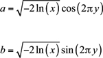
The Box-Muller method can only transform an even number of input values.
The Polar method is similar to the Box-Muller method, but removes the need to compute sine and cosine values. The Polar equations are given by
and
where
q =(2x−1)2 +(2y−1)2
The problem with the Polar method is that q must be less than 1. Any input values that would result in an invalid value must be discarded. Therefore, the number of output values will usually be less than the number of input values. Despite the discarding, the Polar method is as effective as the Box-Muller and generally computes values faster.
The last method is the Moro inversion, which is entirely different from the Box-Muller and Polar methods. It returns one normally distributed value for each uniformly distributed value, and does so by computing the inverse of the cumulative distribution function, or cdf. The cdf is the probability that a random variable is less than or equal to a specific value. You can find more information about Moro’s inversion and the other two methods in The Monte Carlo Programmer’s Guide and API Reference.
Table 18.6 lists all the libmc_rand functions that transform the distribution of numeric sequences. In each case, the input floats must lie between 0 and 1, but may not equal 0 or 1.
Table 18.6. Monte Carlo Functions for Transforming Uniform Sequences into Normal Sequences
Function Name | Purpose |
|---|---|
| Transforms |
| Transforms |
| Transforms |
| Transforms |
| Transforms |
| Transforms |
| Transforms the |
| Transforms the |
| Transforms |
| Transforms |
The Box-Muller functions are identified with bm2 and the Moro inversion functions are identified with mi. Each Box-Muller function operates on an array of uniformly distributed vectors and produces an output array of normally distributed values. The first two Moro inversion functions operate on arrays, and the second two receive individual vectors. The second pair of Moro inversion functions, mc_transform_mi_array_f4 and mc_transform_mi_array_d2, return their output values in a vector.
The last four functions in the table transform number distribution with the Polar method. Their usage is markedly different from the Box-Muller and Moro inversion functions. Each accepts a pointer to a function that generates pseudo-random numbers, and this is necessary because the Polar method discards unsuitable input values. To produce N output values, the Polar functions must call the generation function until all N outputs are produced.
The functions that use the Polar method can be confusing, so the code in Listing 18.3 shows how they’re used in practice. First, the spu_random2 application uses the Mersenne Twister to generate four vector floats containing uniformly distribute values. Then it transforms the uniformly distributed sequence into a normally distributed sequence using the Polar method.
Example 18.3. Transforming Random Numbers: spu_random2.c
#include <stdio.h>
#include <stdlib.h>
#include <spu_intrinsics.h>
#include <sys/time.h>
#include <mc_rand.h>
#include <simdmath.h>

int main() {

   int i, j;

   /* The input and output arrays */
   vector float uniform_vec[4];
   vector float normal_vec[4];

   /* Generate a seed */
   struct timeval time;
   gettimeofday(&time, NULL);

   /* Generate the random numbers */
   mc_rand_mt_init(time.tv_sec);
   mc_rand_mt_0_to_1_array_f4(4, uniform_vec);

   /* Transform the array */
   mc_transform_po_array_f4(4, uniform_vec, normal_vec,
      &mc_rand_mt_0_to_1_f4);

   /* Display the results */
   printf("Uniform Distribution:
");
   for(i=0; i<4; i++)
      for(j=0; j<4; j++)
         printf("%f ", spu_extract(uniform_vec[i], j));

   printf("

Normal Distribution:
");
   for(i=0; i<4; i++)
      for(j=0; j<4; j++)
         printf("%f ", spu_extract(normal_vec[i], j));
   printf("
");
   return 0;
}
The call to mc_transform_po_array_f4 might seem odd at first. The last parameter is a pointer to the function mc_rand_mt_0_to_1_f4, which uses the Mersenne Twister to produce a vector float of uniformly distributed values. If the Polar method can call the generation function, why does it need an input vector of floats? The answer is that the Polar method may need to discard input values, and the Mersenne Twister provides a backup mechanism to make sure that count values are always returned.
This chapter has covered a lot of ground in a small number of pages, and it’s a shame that neither of the topics have received the in-depth treatment they deserve. Multiprecision mathematics and Monte Carlo methods are not only important facets of the SDK, they’re also crucial in cryptography, simulation, and financial modeling. Research in these areas progresses at a rapid pace, so don’t be surprised if these libraries expand beyond their current capabilities.
The functions in the Multiprecision Math library, or libmpm, operate on values whose bit length far exceed any of the normally available datatypes. Many of the functions perform simple arithmetic, but others implement such complex algorithms as modular reduction and exponentiation. These routines are vital in cryptography, and although this chapter presented a basic RSA application, a full appreciation of the libmpm functions requires specialized knowledge in the field of computational mathematics.
The routines in the Monte Carlo library, libmc_rand, make it possible to generate and transform numbers whose properties approach randomness. Some functions generate pseudo-random numbers, whereas others generate quasi-random numbers. Pseudo-random numbers, generated by the Kirkpatrick-Stoll method and the Mersenne Twister, come close to the ideals of independence and identical distribution. Quasi-random numbers aren’t as independent as pseudo-random numbers, but are distributed in such a way as to occupy as much of the range as possible. They’re commonly used in simulations where space filling is a priority.
The transformation functions in libmc_rand accept uniformly distributed number sequences and produce values with a normal probability distribution. The Polar method functions execute faster than the Box-Muller and Moro inversion functions, but they’re more complex to use in code. This is because the Polar method requires that certain input values be discarded before processing.