You’ve compiled and run your application, but the development process doesn’t end there. If runtime errors crop up, you need a way to step through the executable and determine which lines of code produced the errors. The SDK provides two debuggers for this purpose: ppu-gdb and spu-gdb, and both closely resemble GNU’s gdb debugger.
Even if the application runs without errors, it might not meet performance requirements. In this case, you need to locate problems like pipeline stalls, branch miss percentages, and direct memory access (DMA) bus overload. No debugger can give you these statistics, but IBM’s Full-System Simulator for the Cell processor, called SystemSim, provides all this information and more.
This chapter describes the SDK’s debuggers and SystemSim in detail. It explains the tools’ commands and gives examples of how they’re used. Keep in mind, however, that the SDK also provides an integrated development environment (for Linux) that enables point-and-click debugging and simulation. If command lines make you nervous, you may want to proceed to the next chapter.
The concept of debugging is simple: run an application until a specific line of code is reached or a specific condition occurs, then halt. Read the state of the processor and step through succeeding lines. Keep examining the processor’s state until you can determine what’s producing the error.
Just as gcc is the preeminent open source tool for building applications, gdb is the preeminent tool for debugging them. The Cell SDK provides two debuggers, both based on gdb. ppu-gdb debugs applications built for the PPU and spu-gdb debugs applications built for the SPU. Both use the same commands, which are the same commands used by gdb. If you’re already familiar with these commands, you might want to skip to the next section, which describes the Full-System Simulator.
This section concentrates on spu-gdb for three reasons. First, its commands are essentially the same as those used by ppu-gdb. Second, the SPU architecture is simpler than the PPU’s, so it’s easier to analyze its registers and memory. Third, SPUs perform the brunt of the Cell’s number crunching, so it’s very important to get your SPU applications working properly.
A PPU or SPU application can be debugged only if it was compiled with -g and without optimization. The -g option inserts debug information into the executable and makes sure that each line can be executed separately. If you try to debug an optimized application, its breakpoints and watchpoints won’t work correctly.
A typical spu-gdb session consists of seven main stages:
Enter
spu-gdbfollowed by the name of the executable. This starts the debugger.At the
(gdb)prompt, usebreakto create a breakpoint orwatchto create a watchpoint.Enter
run. This executes the application until the breakpoint location is reached or the watchpoint condition becomes valid.When the application halts, use commands such as
infoto examine the state of the processor.Use the
step,next, orcontinuecommands to execute succeeding lines.Repeat previous steps until the bug is discovered. Enter
runto complete the application’s execution.Enter
quitto end the debugger session.
To effectively use spu-gdb from the command line, you need to understand its basic instructions. This discussion divides them into three categories: commands that set breakpoints and watchpoints, commands that read processor information, and commands that control the execution of the application.
Before you can analyze the conditions that cause a bug, you need to halt the application at the right place. Breakpoints are created with the break command, and halt the application when a location in code (line number, function name, instruction address) is reached. Watchpoints are created with watch, and halt the application when a specific condition occurs. Table 4.1 lists these commands and a number of different usages.
Table 4.1. Breakpoint/Watchpoint Commands
Command | Description |
|---|---|
| Halt before line number |
| Halt just as function |
| Halt when the instruction at |
| Halt at location (line or function) |
| Halt at location (line, function, or address) |
| Halt when expression |
| Halt when expression |
For example, break main halts the application as the main function starts and break 20 halts the application as it reaches line 20. The command watch x halts the application when x changes value, and rwatch x halts the application when x is read. The break command can be shortened to b and watch can be shortened to w.
Once the application halts, the next step is to examine the processor’s state. This state information includes variable values, register contents, and data stored in memory. The three basic commands are where, print and info, and Table 4.2 lists them and a few of their variations.
Table 4.2. Debug Information Commands
Command | Description |
|---|---|
| Show current file, function name, and line number |
| Show current file, function name, line number, and local variables |
| Show the current value of variable |
| Show address of variable |
| Show the current value of variable |
| Show the content of register |
| Show address or register containing |
| Show arguments of the current stack frame |
| Display information about the source code being analyzed |
| List all enabled breakpoints |
| List all enabled watchpoints |
If x is a variable in scope, print x command shows its value, and print &x shows its address. The info registers command lists the contents of all the processor’s registers, and info registers num displays the content of register num. If you ever need to get your bearings during the course of a debug session, where full displays the current function, line number, and local variables.
spu-gdb recognizes abbreviated forms of these commands: i for info and p for print. For example, the command i r 20 is the abbreviated form of info registers 20, and displays the contents of Register 20. Similarly, entering p count will tell you the current value of the variable count.
A debug session commonly requires gaining information about the processor at many different points in its operation. This makes it necessary to keep close control over which lines of code are processed. The commands in Table 4.3 provide this control.
Table 4.3. Debug Start/Stop Commands
Command | Description |
|---|---|
| Start the program being debugged |
| Execute the current instruction |
| Execute num instructions |
| Execute the current instruction, return from function call |
| Execute num instructions, return from any function calls |
| Resume program execution |
| Continue until end of current function |
It’s important to understand the difference between step and next. step executes the current instruction and proceeds to the next instruction. If the current instruction is a function call, step enters the function and proceeds to its first line.
next is similar, but if the current instruction is a function call, next executes the function and proceeds to the line after the function call. In other words, step steps into functions and next steps over them. step, next, and continue are commonly abbreviated s, n, and c, respectively.
Now that you’ve seen the spu-gdb commands, it’s time to look at an example of how they’re used in a real debugging session. Listing 4.1 presents the source code to be examined. The compiled application finds prime numbers between 2 and N using the Sieve of Eratosthenes.
Example 4.1. Sieve of Eratosthenes: spu_sieve.c
#include <stdio.h>

#define N 250

int main() {
   int i, j;
   unsigned int num_array[N + 1];
   num_array[0] = num_array[1] = 1;

   /* Set i^2 and further multiples of i to 1 */
   for (i=2; i*i <= N; i++) {
      if (num_array[i] == 0) {
         for (j=i*i; j <= N; j+=i)
            num_array[j] = 1;
      }
   }

   /* Display indices of prime numbers */
   printf("Prime numbers less than %u: ", N);
   for (i=2; i <= N; i++) {
      if (num_array[i] != 1)
         printf("%u ", i);
   }
   printf("
");

   return 0;
}
The first loop iterates through num_array, and if i hasn’t been marked as a composite number, the value of num_array[i2] is marked along with every following num_array value whose index is a multiple of i. The second loop iterates through the array and lists all values of i that haven’t been marked. These are the primes between 2 and the size of num_array.
To demonstrate how the debugger works, the following session creates a breakpoint at the first function, main. It runs to the first line of executable code and steps to the next. It executes ten more lines with next 10, finds its position with where, and sets another breakpoint at Line 19. Finally, the session lists the breakpoints, continues to the second breakpoint, and runs to completion:
% spu-gdb spu_sieve -q
(gdb) break main

Breakpoint 1 at 0x170: file spu_sieve.c, line 8.
(gdb) run

Breakpoint 1, main () at spu_sieve.c:8
8          num_array[0] = num_array[1] = 1;
(gdb) step

11         for (i=2; i*i <= N; i++) {
(gdb) next 10

13               for (j=i*i; j <= N; j+=i)
(gdb) print j

$1 = 10
(gdb) where

#0  main () at spu_sieve.c:13
(gdb) break spu_sieve.c:19

Breakpoint 2 at 0x2a4: file spu_sieve.c, line 19.
(gdb) info breakpoints

Num Type           Disp Enb Address    What
1   breakpoint     keep y   0x00000170 spu_sieve.c:8
        breakpoint already hit 1 time
2   breakpoint     keep y   0x000002a4 spu_sieve.c:19
(gdb) continue

Continuing.

Breakpoint 3, main () at spu_sieve.c:19
19         printf("Prime numbers less than %u: ", N);
(gdb) continue

Continuing.
...Program output...

Program exited normally.
(gdb) quit
When setting breakpoints at line numbers, it’s a good idea to identify the filename, as in the preceding example. Otherwise, the debugger may halt in a source file you hadn’t expected.
The Cell SDK debuggers can assist you in finding the source of an error, but they aren’t as helpful at improving an application’s efficiency. By this I mean reducing branch misses, reducing DMA traffic, and making the best use of a processor’s pipeline. ppu-gdb and spu-gdb can’t provide this kind of low-level information, but IBM’s Full-System Simulator can.
Up to this point, the book’s discussion has centered on building, running, and debugging applications on an actual Cell processor. This section switches gears and focuses on simulating applications with IBM’s Full-System Simulator for the Cell Broadband Engine. This is a powerful tool, and it’s not just for those who can’t access a Cell device; it’s for any developer who wants a thorough understanding of how the Cell processes code.
The simulator, hereafter referred to as SystemSim, gives users nearly absolute oversight of the PPU and all eight SPUs—an experience that PlayStation 3 developers will never otherwise have. Like a debugger, the simulator displays the contents of registers and memory. But it also keeps track of additional data like bus usage, address translation, stack pointer location, and DMA communication.
With SystemSim, you can start the simulated Cell with no operating system whatsoever. This is called standalone mode. If you choose this, there are a few restrictions:
No access to virtual memory operations.
All applications must be statically linked.
Some Linux system calls are unsupported.
The presentation that follows assumes that Linux is installed on the simulated Cell. In this case, the restrictions don’t apply.
SystemSim can be configured to provide cycle accurate timing, which means you can test applications on the simulator with the same confidence as you can with an actual Cell. Further, the simulator keeps track of cycle counts on the PPU, SPUs, and DMA buses, so you can compare the timing on one processing unit to that of another.
SystemSim’s chief drawbacks are that it has too many features and displays too much information. The goal of this section is to provide a basic tour of the simulator’s capabilities, so don’t be concerned if you don’t understand all of it.
IBM originally created SystemSim to provide low-level simulation of its PowerPC line of processors. It isn’t hard-coded for any particular device, but uses a configuration file to specify the processor’s characteristics. In SystemSim terms, this configuration file defines a machine type.
When the Cell SDK simulator starts on a PC running Linux, it reads the configuration file systemsim.tcl in /opt/ibm/systemsim-cell/lib. This file defines the resources, operation, and timing of the Cell processor. By accessing this file, users can configure the parameters of the simulated Cell. For instance, the size of the simulated system memory is set to 256MB, just as in the PS3, but this value can be increased as needed.
SystemSim communicates with the outside world using Tcl (Tool Command Language), and its capabilities can be extended with additional Tcl scripts. When it initializes, SystemSim searches for scripts in the /opt/ibm/systemsim-cell/lib directory and in the common and ppc subdirectories. By looking through these directories, you can see how Tcl scripts access SystemSim. For more information on Tcl, see Appendix E,“A Brief Introduction to Tcl.”
The script that starts the simulator is called systemsim and it’s located in /opt/ibm/systemsim-cell/bin. For the discussion that follows, it’s a good idea to add this directory to your PATH variable and create an environment variable called SYSTEMSIM_TOP that points to /opt/ibm/systemsim-cell. This can be done by inserting the following lines into .bash_profile in your home directory:
export PATH=/opt/ibm/systemsim-cell/bin:$PATH
export SYSTEMSIM_TOP=/opt/ibm/systemsim-cell
Then start the simulator with
systemsim -g -q
The -q option tells SystemSim to run in quiet mode, and the -g tells the simulator to create a GUI. By default, this command invokes the startup script systemsim.tcl in $SYSTEMSIM_TOP/lib/cell. You can access a different startup script by using the -f filename option.
As systemsim.tcl executes, three things happen:
The terminal in which the script was run becomes the simulator’s command window. This sends Tcl commands to the simulator.
A new window is created that communicates with the simulated Cell device. This is the console window.
A graphical panel appears with buttons and folders. Figure 4.1 shows what the panel looks like.

The graphical panel is divided into two sections. On the left, a directory tree presents the resources of the mysim machine (the Cell processor). On the right, a grid of buttons shows the different commands that can be issued to the simulator. Table 4.4 lists each of these buttons and their functions, from top left to bottom right.
Table 4.4. Control Buttons for the Full-System Simulator
Button | Functions |
|---|---|
Advance Cycle | Progress simulation by number of cycles shown in the upper text box |
Go | Starts simulation if it hasn’t begun, continues simulation if it was stopped |
Stop | Pause simulation |
Service GDB | Enable external GDB instance to attach to the simulated program |
Triggers/Breakpoints | Show which triggers and breakpoints are currently valid |
Update GUI | Refresh simulator panel with updated results |
Debug Controls | Allows configuration of debug controls |
Options | Edit settings such as GUI fonts and debugger port |
Emitters | Shows valid emitters for simulated program |
Mode | Specifies whether simulation should run in fast, simple, or cycle mode |
SPU Modes | Specifies whether SPUs should run in instruction, pipeline, or fast mode |
SPE Visualization | Displays histograms of SPU and DMA events |
Track All PCs | Display program counters of all processing elements |
Event Log | Enables collection of log information |
Exit | Ends the simulation and closes GUI |
The first button that concerns us is the Mode button. This controls the precision with which SystemSim simulates the Cell. Click this button and a dialog will present three options: Fast, Simple, and Cycle (see Figure 4.2).

If the Cycle mode is chosen, SystemSim performs cycle-accurate simulation of the Cell’s resources. This provides high-precision measurement but demands a great deal of processing power. It takes a great deal of time to install Linux on the simulated Cell in Cycle mode, so for now, choose the Fast mode.
Now you’re ready to start the simulator. Click the Go button in the panel and the simulator will install Linux on the simulated Cell. When it finishes, the command window and console window will display their command prompts and await your orders. These two windows serve different functions and receive commands in different languages.
When SystemSim starts, the terminal that ran the systemsim script becomes the command window. As Linux finishes booting on the simulated Cell, the command window stops producing output and displays the command prompt: systemsim %. If this prompt isn’t visible at first, select the window and press Enter until it appears. Figure 4.3 shows what the window and its prompt look like.

This window sends commands directly to SystemSim and controls the simulator’s operation. The command language is based on Tcl, and if you enter
puts "Hello command window!"
SystemSim will understand the command and display the string. If you place this command in a file ending in .tcl, such as /tmp/hello.tcl, you can execute the file with the following command:
tclsh /tmp/hello.tcl
These Tcl scripts make it possible to interact with the simulator and other Tcl scripts. It’s a good idea to look through the scripts in $SYSTEMSIM_TOP/common to get an idea of how they work.
The SystemSim console window is different from the command window in many respects. It’s smaller, its font is smaller, and it displays keystrokes more slowly than the command window. Figure 4.4 shows what the console window looks like.

The console window operates more slowly because its input goes through the simulator and into the simulated device. This is an important distinction:The command window sends input to the SystemSim application running on the host system. The console window sends input to a shell on the simulated Cell processor.
Tcl commands won’t work in the console window, but you can run regular Linux shell commands such as cp, ls, and mkdir. The home directory is /root by default, and I recommend that you explore the simulated file system: The executables are in /bin and the devices are in /dev.
The console window lets you transfer files between the host system and the simulated Cell. More important, it allows you to run executables on the simulated Cell. This capability is discussed next.
Cell software development on the simulator generally takes six steps, some of which are optional:
Configure simulation parameters (PPU mode, SPU mode) and identify data collection procedures (triggers, emitters) using the command window.
Build a Cell executable on the host system using the SDK’s cross-development tools.
Transfer the executable and support files from the host system to the simulated Cell using the
callthru sourcecommand in the console window.Run files on the simulated Cell by entering commands in the console window.
Transfer output files from the simulated Cell to the host system using the
callthru sinkcommand in the console window.Use the command window to access data generated during the simulation.
Data collection methods, including triggers and emitters, will be presented shortly. For now, let’s simulate a simple application: the Sieve of Eratosthenes executable from the previous section.
If the host processor isn’t a 64-bit PowerPC, the Cell SDK installer installs packages for cross-development. The tools in these packages run on the host processor but compile code for the Cell. They have the same names (ppu-gcc, spu-gcc) as those described in Chapter 3, “Building Applications for the Cell Processor,” but the compiled executables can’t run directly on the host processor.
Note
At the time of this writing, the directory containing the cross-development tools isn’t added to the PATH environment variable. To ensure that the makefiles work properly, add /opt/cell/toolchain/bin to the PATH variable.
The code for this example can be found in the Chapter4/sieve directory. To build the application, change to this directory and enter make. This invokes the build commands in Makefile, which use the host’s cross-development tools to generate the spu_sieve executable.
The host processor can’t run spu_sieve because it was compiled for the Cell. To transfer the executable to the simulated Cell, you need the callthru command. This command, entered in the console window, transfers files between the host and the simulated device. It can be used in two ways:
where HOST_DIR is a directory on the host system and CELL_DIR is a directory on the simulated Cell. The first command, callthru source, transfers file_name from the host to the simulated device and the second, callthru sink, transfers file_name from the simulated device to the host.
To reduce the size of the pathname on the host, it’s common to move files to the host’s /tmp directory before transferring them to the Cell. Change to the Chapter4/sieve directory and enter
cp spu_sieve /tmp
Then transfer the executable to the simulated device by entering the following command in the console window:
callthru source /tmp/spu_sieve > spu_sieve
The spu_sieve file will be placed in the current directory on the simulated Cell. It’s a good idea to run ls to make sure the transfer completed properly.
If you attempt to run the executable immediately, you’ll receive a permission error. Make the file executable with
chmod +x spu_sieve
and run it by calling ./spu_sieve in the console window. The console will present a list of the prime numbers less than 250.
Optionally, you can transfer spu_sieve back to /tmp on the host by entering the following:
callthru sink /tmp/spu_sieve < spu_sieve
callthru is a vital command in the console window, so it’s important to have a clear understanding of how it’s used.
The Full-System Simulator can do much more than just run Cell applications. To appreciate SystemSim, you need to see the performance data it collects and the different ways you can control how and when the data is collected. This control is an important benefit of using the simulator, and there are two simple ways to take advantage of it:
Enter Tcl profiling commands in the command window.
Insert profiling commands into SPU code. These commands are called checkpoints.
The first method collects performance data throughout the execution of an application. The second method lets you control when the data collection begins and ends.
SPU performance data, collectively called statistics, include the number of instructions executed, the number of cycles run, and the number of pipeline stalls that occurred during the simulation. Appreciating these measurements requires a thorough understanding of the Cell’s architecture, so this discussion just walks through a brief example.
Like the PPU, each SPU has a simulation mode that determines how precisely SystemSim performs its analysis. By default, all SPUs are set to Instruction mode, which means SystemSim doesn’t acquire performance data. To gather statistics, the SPUs need to be in Pipeline mode. Click the SPU Mode button in the graphical panel and select Pipeline for each SPU. Figure 4.5 shows what the SPU mode selection dialog looks like.

If the executable isn’t there already, use callthru to transfer spu_sieve to the simulated Cell. Then complete the following steps:
In the graphical panel, click Stop to pause the simulation.
In the command window, enter
mysim spu 7 stats reset. This clears the simulator’s stored statistics for SPU 7.In the graphical panel, click Go to start the simulation once more.
In the console window, run
./spu_sieve.In the command window, enter
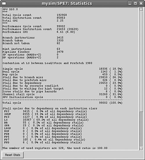
mysim spu 7 stats print. This displays the statistics generated during the execution ofspu_sieve.
Note
This discussion assumes that the operating system chooses SPU 7 to run executables. If this isn’t the case, you’ll need to reenter the commands for the chosen SPU.
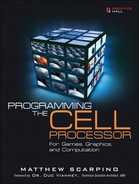
Instead of using mysim spu 7 stats print, you can access SPU statistics by opening the SPE7 folder on the left side of the graphical panel and double-clicking SPUStats. Figure 4.6 shows what the statistics window looks like.
You can also view the contents of SPU memory and the operation of the SPU’s Memory Flow Controller by selecting the corresponding options (SPUMemory and MFC) in the SPE7 directory.
SystemSim makes SPU statistics available to Tcl scripts as array structures. The command needed to access them is
array set myArray [mysim spu n stats export]
where myArray is the name of the array to store the data and n is the SPU being examined. This command is commonly used by SystemSim triggers, which are discussed shortly.
You may only want performance data for a specific portion of an application. In this case, running commands in the command window won’t be sufficient: You need to modify the SPU code in a way that tells the simulator when to start and stop collecting measurements.
Checkpoints are statements in C/C++ code that control when SystemSim collects data. Each checkpoint function is named prof_cpN(), where N is a value between 0 and 31. These functions are treated as no-ops during execution, but the simulator recognizes them for control purposes. Of the 32 checkpoints, 3 have specific purposes:
prof_cp0():Resets the SPU statistics for the SPUprof_cp30():Enables collection of statistics for the SPUprof_cp31():Ends collection of statistics for the SPU
These functions are declared in the header file profile.h, located in $SYSTEMSIM_TOP/include/callthru/spu.
The code in the Chapter4/sieve_check directory implements the same Sieve of Eratosthenes algorithm as in Chapter4/sieve, but inserts checkpoints that reset, start, and stop the simulator’s data collection. Listing 4.2 shows the full code, with the new checkpoint statements in boldface.
Example 4.2. Inserting SystemSim Checkpoints: spu_sieve_check.c
#include <stdio.h>
#include "profile.h"

#define N 250

int main() {
   int i, j;
   unsigned int num_array[N + 1];
   num_array[0] = num_array[1] = 1;

   /* Insert checkpoints */
   prof_cp0();  /* Clear statistics */
   prof_cp30(); /* Start collecting statistics */

   /* Set i^2 and further multiples of i to 1 */
   for (i=2; i*i <= N; i++) {
      if (num_array[i] == 0) {
         for (j=i*i; j <= N; j+=i)
            num_array[j] = 1;
      }
   }

   prof_cp31(); /* Stop collecting statistics */

   /* Display indices of prime numbers */
   printf("Prime numbers less than %u: ", N);
   for (i=2; i <= N; i++) {
      if (num_array[i] != 1)
         printf("%u ", i);
   }
   printf("
");

   return 0;
}
These checkpoints tell the simulator to collect statistics as composite numbers are set to 1, but not before or after. To simulate this application, copy the spu_sieve_check executable to /tmp and enter the following commands in the console window:
callthru source /tmp/spu_sieve_check > spu_sieve_check
chmod +x spu_sieve_check
./spu_sieve_check
To see the statistics generated by the profiled section of code, open the SPE7 directory in the graphical panel and select SPUStats. Alternatively, you can enter the following in the command window:
mysim spu 7 stats print
This displays the same type of metrics as before, but the data represents only the processing that took place between the checkpoints.
Event handling is an important aspect of simulation. If a stack overflow occurs, you need a way to halt the simulation and find out what happened. SystemSim provides triggers for this purpose, and the process of using them consists of two parts:
Identify the conditions SystemSim should monitor.
Tell the simulator what actions it should take when those conditions occur.
The conditions of interest are called trigger events, and the actions are called trigger actions.
SystemSim responds to many different types of trigger events, each represented by a string constant. Table 4.5 lists a number of them, but not all. For the full list of trigger events, enter
mysim trigger display assoc avail
in the SystemSim command window.
Table 4.5. SystemSim Trigger Events
Description | |
|---|---|
| Called when simulation resumes or starts |
| Called when simulation pauses or stops |
| Called when an SPU starts operating |
| Called when an SPU completes operating |
| Called when an SPU starts DMA data transfer |
| Called when an SPU ends a DMA data transfer |
| Called when the SPU reaches a profiling function (prof_cp) |
| Called when the PPU loads an executable object onto the SPU |
| Called when a PPU application executes a callthru |
| Called when the simulator encounters an internal error |
| Called when the simulator encounters a fatal error |
The first six events are straightforward. SIM_START/SIM_STOP respond to the simulator’s operation, SPU_START/SPU_STOP respond to the SPU’s operation, and SPE_DMA_START/SPE_DMA_STOP respond to DMA operations.
The seventh event, SPU_PROF, is particularly important because it responds to checkpoints in SPU code. That is, an SPU_PROF event occurs whenever the simulated device calls one of the prof_cpN functions. By creating triggers for SPU_PROF events, you can send commands to SystemSim whenever a particular line of code is reached. For example, the trigger may halt the simulator at a checkpoint. In this case, the checkpoint acts like a regular breakpoint for debugging.
Trigger actions tell SystemSim what to do when a trigger event occurs. They are implemented as Tcl procedures, described in Appendix E. When SystemSim invokes a trigger action, it passes information about the simulation state into the procedure. This information takes the form of a Tcl list containing a series of name/value pairs.
For example, if the triggering event is SPU_PROF, the list contains six elements:
spu spu_num cycle cycle_num rt trig_num
where spu_num is the number of the simulated SPU, cycle_num is the current cycle count, and trig_num is the number of the checkpoint that caused the event. That is, trig_num contains N in prof_cpN.
Note
The list elements provided for SPU_PROF and other events may change in future releases of SystemSim.
These values can be accessed easily by converting the input list to a Tcl array. This is done with the array set command. For example, if the list values are placed in an array called args and the triggering event is SPU_PROF, the spu_num and trig_num elements can be accessed using $args(spu) or $args(rt).
Besides simulation information, you can send data to a trigger action from the command window. If a Tcl variable is defined on the command line, trigger actions will be able to access it as a global variable. For example, if a command defines stat_count with
set stat_count 0
a trigger action will be able to access the variable with the declaration
global stat_count
If the trigger action changes the value of stat_count, the updated result be available from the command line.
A common purpose of trigger actions is to halt the simulated Cell so that the user can examine its state. This is done with the simstop command. Another purpose is to collect performance data, and this is performed with the command
array set myArray [mysim spu n stats export]
where myArray is the Tcl array that will store the SPU metrics, and n is the number of the SPU being examined.
For each trigger action you create, you need to load the Tcl script into memory and associate the action with an event. There are two steps involved:
Run
source trig_script, wheretrig_scriptis the path to the trigger action script. This tells SystemSim to read your trigger script into memory.Execute
mysim trigger set assoc event_name trig_procin the command window, whereevent_nameis an event constant, andtrig_procis a procedure intrig_script. This command associates the trigger with the event.
For example, suppose you created a trigger script called start_script.tcl and placed it in the host’s /tmp directory. This script contains a trigger action called start_proc and you want this procedure to be called whenever an SPU starts. The first step is to source the script with
source /tmp/start_script.tcl
Then, to associate this trigger action with the SPU_START event, execute the following in the command window:
mysim trigger set assoc "SPU_START" start_proc
You can verify the association by clicking Triggers/Breakpoints in the graphical panel and looking at the available triggers. As the simulation runs, SystemSim will monitor the start of an SPU’s operation and execute spu_proc when the event takes place.
Listing 4.3 presents an example trigger action that responds to SPU_PROF trigger events. When this event occurs, the trigger action checks the number (0, 30, or 31) that corresponds to the prof_cp0, prof_cp30, and prof_cp31 functions. If the number equals 31, the action reads the simulator’s SPU statistics and prints the statistics corresponding to the pipeline stall cycles and branch instructions. The trigger’s output is sent to the command window.
Example 4.3. SPU Profile Trigger: prof_trigger.tcl
proc print_prof { arg_list } {

   # Create array from the input list
   array set arg_array $arg_list

   # Check for end of statistic collection
   if {$arg_array(rt) == 31} {

      # Read the SPU statistics
      array set stat_array [ mysim spu $arg_array(spu) stats export ]

      puts "Pipe dependent stall cycles:
         $stat_array(pipe_dep_stall_cycles)"

      puts "Branch instruction count:
         $stat_array(BR_inst_count)"
   }
}
The array set command creates an array called arg_array from the incoming list of arguments. If the trigger number, accessed with $arg_array(rt), equals 31, the trigger places the SPU statistics in an array called stat_array. Then it displays two statistics: the number of pipeline-dependent stall cycles and the number of branch instructions. The first statistic is identified by the pipe_dep_stall_cycles index, and the second is identified by BR_inst_count.
If prof_trigger.tcl is placed in trig_dir, the following commands (in the command window) will load the script into SystemSim and associate it with the SPU_PROF event:
source trig_dir/prof_trigger.tclmysim trigger set assoc "SPU_PROF" print_prof
Assuming spu_sieve_check is in the host’s /tmp directory, the following commands (in the console window) will run the executable:
As the application processes the checkpoints, SystemSim will invoke the print_prof procedure. When the prof_cp31() checkpoint is reached, print_prof will display the number of pipeline-dependent stall cycles and the number of branch instructions executed between prof_cp30() and prof_cp31().
SystemSim can be configured to provide (or emit) processor information when specific events occur. The simulator provides this information in the form of data structures called emitter records, and they can be read by C/C++ executables called emitter readers. This operation is quite different from triggers, in which SystemSim sends processing data to Tcl procedures in the form of Tcl lists.
But like triggers, configuring emitters is a two-step process:
Create Tcl commands that tell SystemSim to produce emitter records when simulation events occur.
Create a C/C++ application to read and process the records produced by SystemSim.
You can obtain more information about the processor with emitters than you can with triggers, but it’s more complex to code the event handling procedures. Also, the Tcl code must be processed as SystemSim starts up instead of being loaded into memory during regular operation.
Emitters enable you to monitor many more event types than triggers, including memory accesses, instruction prefetches, segment table lookups, and hits and misses for the L1 cache (both the instruction and data cache). Table 4.6 presents a subset of these events, and you can access the full list by running simemit list on the SystemSim command line.
Table 4.6. Emitter Event Types
Event | Tag Value | Description |
|---|---|---|
|
| Read from system memory |
|
| Write to system memory |
|
| Accesses to the hard disk |
|
| SPU instruction processing |
|
| SPU read operations |
|
| SPU write operations |
|
| Object code placed in SPU memory |
|
| Beginning of SPU execution |
|
| End of SPU execution |
|
| Enter idle state |
|
| Leave idle state |
|
| Completion of SPU-initiated transfer |
|
| Completion of PPU-initiated transfer |
|
| Marks the beginning of the event data |
|
| Marks the end of the event data |
Many emitter events begin with Apu, which is an older term for the SPU. In addition to those listed, other events respond to pipeline activity, threads, interrupts, and kernel operation. The importance of the tag values in the second column will be explained shortly.
To configure SystemSim to respond to emitter events, you need to perform three steps:
Identify events of interest with
simemit set.Identify the number of emitter readers with
ereader expect.Identify the name of each emitter reader with
ereader start.
These Tcl commands must be processed as SystemSim starts. If you run them afterward, SystemSim won’t produce emitter records for the events.
The simemit set command tells SystemSim which events to monitor. For example, to tell the simulator to produce an emitter record related to the Apu_Task_Start event, you’d use the following:
simemit set "Apu_Task_Start" 1
The 1 value tells SystemSim to produce a record when the SPU starts execution. To verify that this was configured properly, enter simemit list and check the value of {Apu_Task_Start}.
In addition to identifying processor events, you need to tell SystemSim to provide information related to the Header_Record and Footer_Record events. This enables an emitter reader to recognize the start and end of emitter data. The commands
simemit set "Header_Record" 1
simemit set "Footer_Record" 1
must be executed when configuring emitter events.
Just as simemit identifies events of interest, ereader tells SystemSim about the application or applications that will be waiting for emitter records. ereader expect specifies the number of applications that will be collecting information. If there are two emitter readers, the command is as follows:
ereader expect 2
The command ereader start identifies the emitter readers that will receive event data. This command requires a number of arguments: the full path of the C/C++ executable, the simulator process ID, and any additional arguments for the executable. The process ID can be obtained by accessing the global pid variable. For example, the following command tells SystemSim to start the emitter reader read_data with the global process ID:
ereader start /home/mscarpino/ereaders/read_data [pid]
Listing 4.4 tells SystemSim to monitor the Apu_Mem_Read event and start the eread executable to process event records. More events can be monitored by adding more simemit set commands.
Example 4.4. Emitter Configuration: emit_conf.tcl
proc emit_conf {} {

   # The array of environment variables
   global env

   # Identify the four events to be monitored
   simemit set "Header_Record" 1
   simemit set "Footer_Record" 1
   simemit set "Apu_Mem_Read" 1

   # Configure the event reader
   ereader expect 1
   ereader start $env(SYSTEMSIM_TOP)/Chapter4/emitter/eread [pid]
}

# Start emitter processing
if { [catch {emit_conf} output] } {
   puts "Error!  emitter reader failed to start"
   puts $output
} else {
   puts "Emitter reader started!"
}
The commands in Listing 4.4 must be executed as SystemSim starts up. A simple way to make sure this happens is to append the content of emit_conf.tcl to the end of systemsim.tcl, which is located in the $SYSTEMSIM_TOP/lib/cell directory. Then, when SystemSim starts, you should see Emitter reader started! in the command window.
These commands tell SystemSim that the eread executable will read the emitter records produced by the simulator. Therefore, the next crucial step is to code and compile the eread executable.
Tcl scripts configure event handling, but the applications that receive events, called emitter readers, are regular executables. These executables read the data produced by SystemSim, which is packaged in data structures of type EMIT_DATA. SystemSim produces an EMIT_DATA structure for each event of interest in the order in which the events occurred. This sequence starts with a header EMIT_DATA structure and ends with a footer EMIT_DATA structure.
EMIT_DATA is a union of many C structs, and each struct is associated with a specific event. The declaration of the EMIT_DATA union is given as follows:
union emit_data {
   PATH_INFO path;
   CONFIG_INFO config;
   LOAD_INFO load;
   MMAP_INFO kernmmap;
   IO_INFO io;
   DISK_INFO disk;
   INST_INFO inst;
   CACHE_INFO cache;
   CACHE_OP_INFO cache_op;
   HEADER header;
   MSR_INFO msr;
   LPIDR_INFO lpidr;
   IDLE_INFO idle;
   PID_INFO pid;
   PAGE_INFO page;
   ERAT_INFO erat;
   IDLE_ENTER_INFO idle_enter;
   IDLE_EXIT_INFO idle_exit;
   SUPERVISOR_MODE_ENTER_INFO enter_super_mode;
   SUPERVISOR_MODE_EXIT_INFO exit_super_mode;
   TLB_INFO tlb;
   SLB_INFO slb;
   INTERRUPT_INFO interrupt;
   KERNEL_STARTED_INFO kernel_status;
   KERNEL_THREAD_INFO kernel_thread;
   BUS_WAIT_INFO bus_wait;

#ifdef MCONFIG_SPU
#include "emitter/sti_emitter_union_t.h"
#endif /* #ifdef MCONFIG_SPU */

#ifdef CONFIG_ENERGY_SIMULATION
   PERIODIC_POWER_INFO periodic_power;
   POWER_COMPOUND_EVENT_INFO power_compound_event;
   POWER_BASIC_EVENT_INFO power_basic_event;
#endif /* #ifdef CONFIG_ENERGY_SIMULATION */

   STATS_ANNOTATION_INFO   annotation;
   TRANS_INFO              trans;
   MTRACE_INFO             mtrace;
};
typedef union emit_data EMIT_DATA;
For example, the fourth struct in the union is MMAP_INFO, which contains information about memory-mapped files. It’s declaration in emitter_data_t.h is given as
struct mmap_info {
   EMIT_HEAD head;
   char pathname[MAX_EMITTER_PATHNAME];
   uint64 eaddr;
   int len;
   int prot;
   int flags;
   int file_offset;
};
typedef struct mmap_info MMAP_INFO;
The sti_emitter_union_data_t.h header will be included in EMIT_DATA union if MCONFIG_SPU is defined. This header provides additional data structures declared in sti_emitter_data_t.h. These structs contain information related to DMA, pipeline operation, and SPU statistics. If CONFIG_ENERGY_SIMULATION is defined, three structures will be available that provide information related to simulated power consumption. This is an exciting topic, but beyond the scope of this book.
Each structure in the EMIT_DATA declaration has a different set of fields, but the first field is always EMIT_HEAD. The EMIT_HEAD struct provides basic information about the processing environment and its declaration in emitter_data_t.h is given as
struct emit_head {
   uint8 tag;    /* Identifies the structure type */
   uint8 cpu;    /* Identifies the running CPU */
   uint8 thread; /* Identifies the current thread */
   uint8 mcm;
   uint8 pad[4]; /* Ensure structure is 8-byte aligned */
   uint64 seqid;
   uint64 timestamp;
};
typedef struct emit_head EMIT_HEAD;
One of the most important fields in EMIT_HEAD is tag, which takes one of the tag values listed in the second column of Table 4.6. For example, if tag equals TAG_DISK_REQ, it means the data structure contains information related to the Disk_Requests event.
The EMIT_HEAD header data isn’t related to the HEADER event in EMIT_DATA or the Header_Record event in Table 4.6. This can be confusing, but the next subsection clarifies how headers and events are accessed in code.
As explained earlier, the ereader start command associates emitter readers with a process ID. As SystemSim runs, each reader starts a processing cycle that consists of the following stages:
Attach to the simulator’s shared memory buffer identified by the process ID.
Wait for the simulator to produce
EMIT_DATAobjects.Read the header of each incoming
EMIT_DATAobject.Process the object depending on the header’s
tagvalue.Receive and process further
EMIT_DATAobjects untiltagequalsTAG_FOOTER.Detach the reader and terminate operation.
Common EMIT_DATA processing tasks include getting timestamps from the events of interest, accessing the program counter to determine where an event occurred in code, and printing the results to a file using fprintf.
These stages are controlled by functions in emitter_reader.c, located in $SYSTEMSIM_TOP/emitter. Table 4.7 lists each and its corresponding stage.
Table 4.7. Functions in the Emitter Reader API
Stage | Function | Description |
|---|---|---|
1 |
| Attach the reader using the process ID and return a value for |
2 |
| Wait until an |
3 |
| Increment the pointer to point to the next |
3 |
| Return a pointer to the current |
3 |
| Return a pointer to the first |
3 |
| Return a pointer to the |
6 |
| Detach the reader and free shared memory buffer |
The EMITTER_CONTROLS structure holds the data generated by SystemSim event processing. This data includes the array of EMIT_DATA objects and an array of emitter readers. The first function, EMIT_AttachReader, accepts a pointer to this structure and the process ID. It returns an integer that uniquely identifies the emitter reader. This value is referred to as rdr in the functions that follow.
The rest of the Emitter API functions are straightforward, and most are used to provide access to the array of EMIT_DATA objects. EMIT_AdvanceCurrent increments the array index, EMIT_CurrentEntry returns the current EMIT_DATA object, EMIT_FirstEntry returns the first object in the array, and EMIT_GetEntry returns the EMIT_DATA object at a specified index.
The best way to understand these functions is to use them in code. Listing 4.5 presents an emitter reader that attaches to the SystemSim process, waits for EMIT_DATA objects corresponding to SPU memory access, and prints output to a file called emit.dat.
Example 4.5. Emitter Reader Example: eread.c
#define MCONFIG_SPU          1
#define MCONFIG_STI_EMITTER  1

#include "common/mambo.h"
#include "emitter/emit_collector.h"
#include "trans_id.h"
#include <memory.h>

EMITTER_CONTROLS eControl;

int main (int argc, char **argv) {

   int        pid   = 0;
   EMIT_DATA  *ePtr = NULL;
   FILE       *fp   = NULL;

   /* Obtain the process id */
   pid = atoi(argv[1]);

   /* Open the output file */
   if ((fp = fopen("emit.dat", "w")) == NULL) {
      fprintf(stderr, "Cannot open emit.dat
");
      exit(-1);
   }

   /* Attach to the simulator and wait */
   int rdr = EMIT_AttachReader(pid, &eControl, 0, TRUE);
   if (rdr == -1) {
      fprintf(stderr,  "ERROR: Failed to attach reader
");
      return(0);
   }

   EMIT_ReadyWait(&eControl, rdr, TRUE);

   /* Cycle through EMIT_DATA objects */
   do {
      EMIT_AdvanceCurrent(&eControl, rdr);
      ePtr = EMIT_CurrentEntry(&eControl, rdr);

      switch (ePtr->header.head.tag) {

         /* Respond to SPU memory access */
         case TAG_APU_MEMREAD:
            fprintf(fp, "SPU memory read value: %lld
",
               ePtr->apu_mem.value);
            break;

         default:
            break;
      }
   } while (ePtr->header.head.tag != TAG_FOOTER);

   /* Detach the reader and terminate operation */
   EMIT_Quit(&eControl, rdr, TRUE);
   fclose(fp);
   return(1);
}
The relationship between Tcl event configuration, event tags, and EMIT_DATA structures can be confusing, so let’s be clear about what’s going on:
The Tcl script tells SystemSim to provide data when the
Apu_Mem_Readevent occurs.The tag corresponding to
Apu_Mem_ReadisTAG_APU_MEMREAD. Theswitch-casestatement examines the header data of each incomingEMIT_DATAstructure to see whether it matchesTAG_APU_MEMREAD.If the header data matches this tag, the code accesses the
valuefield contained in theapu_memdata structure. This value is written into a file called emit.dat.
After building the eread executable, place it in $SYSTEMSIM_TOP/Chapter4/emitter. In the console window, transfer the spu_sieve executable to the simulated Cell, change the executable’s permission, and run the executable.
If everything works correctly, SystemSim will produce emitter records for Apu_Mem_Read events and call on the emitter reader, eread, to process them. This reader creates a file called emit.dat and places it in the $SYSTEMSIM_TOP/bin directory. If you open this file, you should find a long series of read values corresponding to the SPU’s memory accesses during the execution of spu_sieve.
The Cell processor is a complex device, and it takes effort to examine how applications are executed. The SDK provides three tools that make this process easier: ppu-gdb, spu-gdb, and the Full-System Simulator (SystemSim). This chapter has focused on the latter two and has described the operation of spu-gdb and SystemSim in depth.
spu-gdb is based on the GNU debugger, gdb, and responds to the same set of commands. It provides capabilities for breakpoints, watchpoints, instruction stepping, and displaying registers and variable values. Its usage boils down to two steps: run the executable until it reaches a specific section of code, and then examine the processor’s state. This process may need to be repeated until the nature of the bug is discovered.
The Full-System Simulator is a powerful tool that creates a simulated Cell processor and makes it possible to run and analyze simulated applications. In addition to displaying the contents of a processor’s registers and memory, it collects performance metrics related to the processor’s operation. The nature of the simulator’s data acquisition can be controlled with checkpoints, triggers, and emitters.
The tools described in this chapter provide a great deal of power, but they’re not particularly easy to use. The next chapter describes the Cell SDK integrated development environment, which makes it possible to build, debug, and simulate applications using a simpler point-and-click methodology.