In the previous chapters, you learned about the essential machine learning algorithms for classification and how to get our data into shape before we feed it into those algorithms. Now, it's time to learn about the best practices of building good machine learning models by fine-tuning the algorithms and evaluating the performance of the models. In this chapter, we will learn how to do the following:

• Assess the performance of machine learning models
• Diagnose the common problems of machine learning algorithms
• Fine-tune machine learning models
• Evaluate predictive models using different performance metrics

Streamlining workflows with pipelines

When we applied different preprocessing techniques in the previous chapters, such as standardization for feature scaling in Chapter 4, Building Good Training Datasets – Data Preprocessing, or principal component analysis for data compression in Chapter 5, Compressing Data via Dimensionality Reduction, you learned that we have to reuse the parameters that were obtained during the fitting of the training data to scale and compress any new data, such as the examples in the separate test dataset. In this section, you will learn about an extremely handy tool, the Pipeline class in scikit-learn. It allows us to fit a model including an arbitrary number of transformation steps and apply it to make predictions about new data.

Loading the Breast Cancer Wisconsin dataset

In this chapter, we will be working with the Breast Cancer Wisconsin dataset, which contains 569 examples of malignant and benign tumor cells. The first two columns in the dataset store the unique ID numbers of the examples and the corresponding diagnoses (M = malignant, B = benign), respectively. Columns 3-32 contain 30 real-valued features that have been computed from digitized images of the cell nuclei, which can be used to build a model to predict whether a tumor is benign or malignant. The Breast Cancer Wisconsin dataset has been deposited in the UCI Machine Learning Repository, and more detailed information about this dataset can be found at https://archive.ics.uci.edu/ml/datasets/Breast+Cancer+Wisconsin+(Diagnostic).

df = pd.read_csv(
     'https://archive.ics.uci.edu/ml/'
     'machine-learning-databases'
     '/breast-cancer-wisconsin/wdbc.data',
     header=None)

df = pd.read_csv(
     'your/local/path/to/wdbc.data',
     header=None)

In this section, we will read in the dataset and split it into training and test datasets in three simple steps:

1. We will start by reading in the dataset directly from the UCI website using pandas:

   >>> import pandas as pd
   >>> df = pd.read_csv('https://archive.ics.uci.edu/ml/'
   ...                  'machine-learning-databases'
   ...                  '/breast-cancer-wisconsin/wdbc.data',
   ...                  header=None)
   

2. Next, we will assign the 30 features to a NumPy array, X. Using a LabelEncoder object, we will transform the class labels from their original string representation ('M' and 'B') into integers:

   >>> from sklearn.preprocessing import LabelEncoder
   >>> X = df.loc[:, 2:].values
   >>> y = df.loc[:, 1].values
   >>> le = LabelEncoder()
   >>> y = le.fit_transform(y)
   >>> le.classes_
   array(['B', 'M'], dtype=object)
   

   After encoding the class labels (diagnosis) in an array, y, the malignant tumors are now represented as class 1, and the benign tumors are represented as class 0, respectively. We can double-check this mapping by calling the transform method of the fitted LabelEncoder on two dummy class labels:

   >>> le.transform(['M', 'B'])
   array([1, 0])
   

3. Before we construct our first model pipeline in the following subsection, let's divide the dataset into a separate training dataset (80 percent of the data) and a separate test dataset (20 percent of the data):

   >>> from sklearn.model_selection import train_test_split
   >>> X_train, X_test, y_train, y_test = 
   ...     train_test_split(X, y,
   ...                      test_size=0.20,
   ...                      stratify=y,
   ...                      random_state=1)
   

Combining transformers and estimators in a pipeline

In the previous chapter, you learned that many learning algorithms require input features on the same scale for optimal performance. Since the features in the Breast Cancer Wisconsin dataset are measured on various different scales, we will standardize the columns in the Breast Cancer Wisconsin dataset before we feed them to a linear classifier, such as logistic regression. Furthermore, let's assume that we want to compress our data from the initial 30 dimensions onto a lower two-dimensional subspace via principal component analysis (PCA), a feature extraction technique for dimensionality reduction that was introduced in Chapter 5, Compressing Data via Dimensionality Reduction.

Instead of going through the model fitting and data transformation steps for the training and test datasets separately, we can chain the StandardScaler, PCA, and LogisticRegression objects in a pipeline:

>>> from sklearn.preprocessing import StandardScaler
>>> from sklearn.decomposition import PCA
>>> from sklearn.linear_model import LogisticRegression
>>> from sklearn.pipeline import make_pipeline
>>> pipe_lr = make_pipeline(StandardScaler(),
...                         PCA(n_components=2),
...                         LogisticRegression(random_state=1,
...                                            solver='lbfgs'))
>>> pipe_lr.fit(X_train, y_train)
>>> y_pred = pipe_lr.predict(X_test)
>>> print('Test Accuracy: %.3f' % pipe_lr.score(X_test, y_test))
Test Accuracy: 0.956

The make_pipeline function takes an arbitrary number of scikit-learn transformers (objects that support the fit and transform methods as input), followed by a scikit-learn estimator that implements the fit and predict methods. In our preceding code example, we provided two transformers, StandardScaler and PCA, and a LogisticRegression estimator as inputs to the make_pipeline function, which constructs a scikit-learn Pipeline object from these objects.

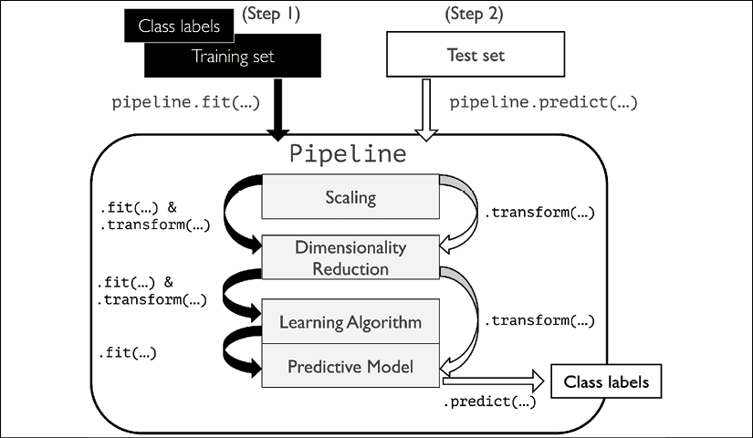
We can think of a scikit-learn Pipeline as a meta-estimator or wrapper around those individual transformers and estimators. If we call the fit method of Pipeline, the data will be passed down a series of transformers via fit and transform calls on these intermediate steps until it arrives at the estimator object (the final element in a pipeline). The estimator will then be fitted to the transformed training data.

When we executed the fit method on the pipe_lr pipeline in the preceding code example, StandardScaler first performed fit and transform calls on the training data. Second, the transformed training data was passed on to the next object in the pipeline, PCA. Similar to the previous step, PCA also executed fit and transform on the scaled input data and passed it to the final element of the pipeline, the estimator.

Finally, the LogisticRegression estimator was fit to the training data after it underwent transformations via StandardScaler and PCA. Again, we should note that there is no limit to the number of intermediate steps in a pipeline; however, the last pipeline element has to be an estimator.

Similar to calling fit on a pipeline, pipelines also implement a predict method. If we feed a dataset to the predict call of a Pipeline object instance, the data will pass through the intermediate steps via transform calls. In the final step, the estimator object will then return a prediction on the transformed data.

The pipelines of the scikit-learn library are immensely useful wrapper tools, which we will use frequently throughout the rest of this book. To make sure that you've got a good grasp of how the Pipeline object works, please take a close look at the following illustration, which summarizes our discussion from the previous paragraphs:

Using k-fold cross-validation to assess model performance

One of the key steps in building a machine learning model is to estimate its performance on data that the model hasn't seen before. Let's assume that we fit our model on a training dataset and use the same data to estimate how well it performs on new data. We remember from the Tackling overfitting via regularization section in Chapter 3, A Tour of Machine Learning Classifiers Using scikit-learn, that a model can suffer from underfitting (high bias) if the model is too simple, or it can overfit the training data (high variance) if the model is too complex for the underlying training data.

To find an acceptable bias-variance tradeoff, we need to evaluate our model carefully. In this section, you will learn about the common cross-validation techniques holdout cross-validation and k-fold cross-validation, which can help us to obtain reliable estimates of the model's generalization performance, that is, how well the model performs on unseen data.

The holdout method

A classic and popular approach for estimating the generalization performance of machine learning models is holdout cross-validation. Using the holdout method, we split our initial dataset into separate training and test datasets—the former is used for model training, and the latter is used to estimate its generalization performance. However, in typical machine learning applications, we are also interested in tuning and comparing different parameter settings to further improve the performance for making predictions on unseen data. This process is called model selection, with the name referring to a given classification problem for which we want to select the optimal values of tuning parameters (also called hyperparameters). However, if we reuse the same test dataset over and over again during model selection, it will become part of our training data and thus the model will be more likely to overfit. Despite this issue, many people still use the test dataset for model selection, which is not a good machine learning practice.

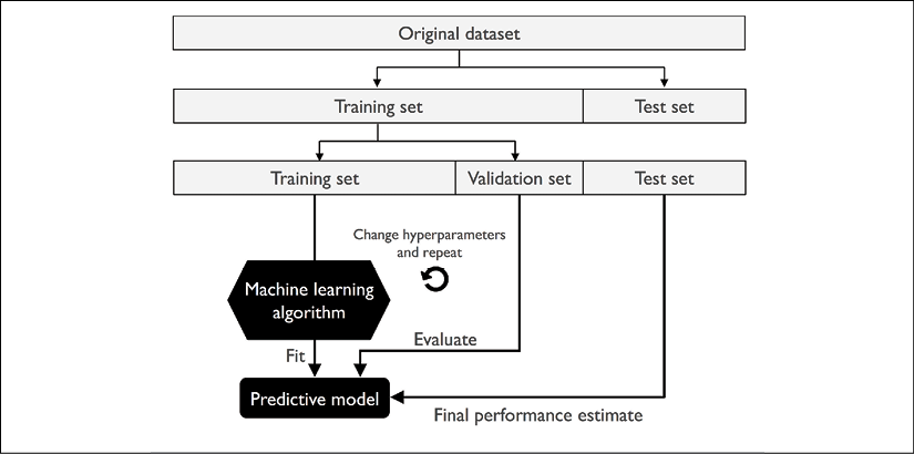
A better way of using the holdout method for model selection is to separate the data into three parts: a training dataset, a validation dataset, and a test dataset. The training dataset is used to fit the different models, and the performance on the validation dataset is then used for the model selection. The advantage of having a test dataset that the model hasn't seen before during the training and model selection steps is that we can obtain a less biased estimate of its ability to generalize to new data. The following figure illustrates the concept of holdout cross-validation, where we use a validation dataset to repeatedly evaluate the performance of the model after training using different hyperparameter values. Once we are satisfied with the tuning of hyperparameter values, we estimate the model's generalization performance on the test dataset:

A disadvantage of the holdout method is that the performance estimate may be very sensitive to how we partition the training dataset into the training and validation subsets; the estimate will vary for different examples of the data. In the next subsection, we will take a look at a more robust technique for performance estimation, k-fold cross-validation, where we repeat the holdout method k times on k subsets of the training data.

K-fold cross-validation

In k-fold cross-validation, we randomly split the training dataset into k folds without replacement, where k – 1 folds are used for the model training, and one fold is used for performance evaluation. This procedure is repeated k times so that we obtain k models and performance estimates.

We then calculate the average performance of the models based on the different, independent test folds to obtain a performance estimate that is less sensitive to the sub-partitioning of the training data compared to the holdout method. Typically, we use k-fold cross-validation for model tuning, that is, finding the optimal hyperparameter values that yield a satisfying generalization performance, which is estimated from evaluating the model performance on the test folds.

Once we have found satisfactory hyperparameter values, we can retrain the model on the complete training dataset and obtain a final performance estimate using the independent test dataset. The rationale behind fitting a model to the whole training dataset after k-fold cross-validation is that providing more training examples to a learning algorithm usually results in a more accurate and robust model.

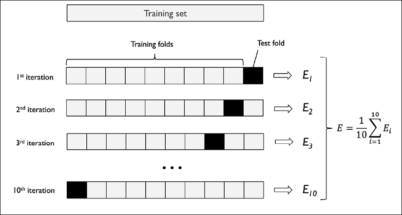
Since k-fold cross-validation is a resampling technique without replacement, the advantage of this approach is that each example will be used for training and validation (as part of a test fold) exactly once, which yields a lower-variance estimate of the model performance than the holdout method. The following figure summarizes the concept behind k-fold cross-validation with k = 10. The training dataset is divided into 10 folds, and during the 10 iterations, nine folds are used for training, and one fold will be used as the test dataset for the model evaluation.

Also, the estimated performances, (for example, classification accuracy or error), for each fold are then used to calculate the estimated average performance, E, of the model:

A good standard value for k in k-fold cross-validation is 10, as empirical evidence shows. For instance, experiments by Ron Kohavi on various real-world datasets suggest that 10-fold cross-validation offers the best tradeoff between bias and variance (A Study of Cross-Validation and Bootstrap for Accuracy Estimation and Model Selection, Kohavi, Ron, International Joint Conference on Artificial Intelligence (IJCAI), 14 (12): 1137-43, 1995).

However, if we are working with relatively small training sets, it can be useful to increase the number of folds. If we increase the value of k, more training data will be used in each iteration, which results in a lower pessimistic bias toward estimating the generalization performance by averaging the individual model estimates. However, large values of k will also increase the runtime of the cross-validation algorithm and yield estimates with higher variance, since the training folds will be more similar to each other. On the other hand, if we are working with large datasets, we can choose a smaller value for k, for example, k = 5, and still obtain an accurate estimate of the average performance of the model while reducing the computational cost of refitting and evaluating the model on the different folds.

A slight improvement over the standard k-fold cross-validation approach is stratified k-fold cross-validation, which can yield better bias and variance estimates, especially in cases of unequal class proportions, which has also been been shown in the same study by Ron Kohavi referenced previously in this section. In stratified cross-validation, the class label proportions are preserved in each fold to ensure that each fold is representative of the class proportions in the training dataset, which we will illustrate by using the StratifiedKFold iterator in scikit-learn:

>>> import numpy as np
>>> from sklearn.model_selection import StratifiedKFold
>>> kfold = StratifiedKFold(n_splits=10).split(X_train, y_train)
>>> scores = []
>>> for k, (train, test) in enumerate(kfold):
...     pipe_lr.fit(X_train[train], y_train[train])
...     score = pipe_lr.score(X_train[test], y_train[test])
...     scores.append(score)
...     print('Fold: %2d, Class dist.: %s, Acc: %.3f' % (k+1,
...           np.bincount(y_train[train]), score))
Fold:  1, Class dist.: [256 153], Acc: 0.935
Fold:  2, Class dist.: [256 153], Acc: 0.935
Fold:  3, Class dist.: [256 153], Acc: 0.957
Fold:  4, Class dist.: [256 153], Acc: 0.957
Fold:  5, Class dist.: [256 153], Acc: 0.935
Fold:  6, Class dist.: [257 153], Acc: 0.956
Fold:  7, Class dist.: [257 153], Acc: 0.978
Fold:  8, Class dist.: [257 153], Acc: 0.933
Fold:  9, Class dist.: [257 153], Acc: 0.956
Fold: 10, Class dist.: [257 153], Acc: 0.956
>>> print('
CV accuracy: %.3f +/- %.3f' %
...      (np.mean(scores), np.std(scores)))
CV accuracy: 0.950 +/- 0.014

First, we initialized the StratifiedKFold iterator from the sklearn.model_selection module with the y_train class labels in the training dataset, and we specified the number of folds via the n_splits parameter. When we used the kfold iterator to loop through the k folds, we used the returned indices in train to fit the logistic regression pipeline that we set up at the beginning of this chapter. Using the pipe_lr pipeline, we ensured that the examples were scaled properly (for instance, standardized) in each iteration. We then used the test indices to calculate the accuracy score of the model, which we collected in the scores list to calculate the average accuracy and the standard deviation of the estimate.

Although the previous code example was useful to illustrate how k-fold cross-validation works, scikit-learn also implements a k-fold cross-validation scorer, which allows us to evaluate our model using stratified k-fold cross-validation less verbosely:

>>> from sklearn.model_selection import cross_val_score
>>> scores = cross_val_score(estimator=pipe_lr,
...                          X=X_train,
...                          y=y_train,
...                          cv=10,
...                          n_jobs=1)
>>> print('CV accuracy scores: %s' % scores)
CV accuracy scores: [ 0.93478261  0.93478261  0.95652174
                      0.95652174  0.93478261  0.95555556
                      0.97777778  0.93333333  0.95555556
                      0.95555556]
>>> print('CV accuracy: %.3f +/- %.3f' % (np.mean(scores),
...       np.std(scores)))
CV accuracy: 0.950 +/- 0.014

An extremely useful feature of the cross_val_score approach is that we can distribute the evaluation of the different folds across multiple central processing units (CPUs) on our machine. If we set the n_jobs parameter to 1, only one CPU will be used to evaluate the performances, just like in our StratifiedKFold example previously. However, by setting n_jobs=2, we could distribute the 10 rounds of cross-validation to two CPUs (if available on our machine), and by setting n_jobs=-1, we can use all available CPUs on our machine to do the computation in parallel.

Debugging algorithms with learning and validation curves

In this section, we will take a look at two very simple yet powerful diagnostic tools that can help us to improve the performance of a learning algorithm: learning curves and validation curves. In the next subsections, we will discuss how we can use learning curves to diagnose whether a learning algorithm has a problem with overfitting (high variance) or underfitting (high bias). Furthermore, we will take a look at validation curves that can help us to address the common issues of a learning algorithm.

Diagnosing bias and variance problems with learning curves

If a model is too complex for a given training dataset—there are too many degrees of freedom or parameters in this model—the model tends to overfit the training data and does not generalize well to unseen data. Often, it can help to collect more training examples to reduce the degree of overfitting.

However, in practice, it can often be very expensive or simply not feasible to collect more data. By plotting the model training and validation accuracies as functions of the training dataset size, we can easily detect whether the model suffers from high variance or high bias, and whether the collection of more data could help to address this problem. But before we discuss how to plot learning curves in scikit-learn, let's discuss those two common model issues by walking through the following illustration:

The graph in the upper-left shows a model with high bias. This model has both low training and cross-validation accuracy, which indicates that it underfits the training data. Common ways to address this issue are to increase the number of parameters of the model, for example, by collecting or constructing additional features, or by decreasing the degree of regularization, for example, in support vector machine (SVM) or logistic regression classifiers.

The graph in the upper-right shows a model that suffers from high variance, which is indicated by the large gap between the training and cross-validation accuracy. To address this problem of overfitting, we can collect more training data, reduce the complexity of the model, or increase the regularization parameter, for example.

For unregularized models, it can also help to decrease the number of features via feature selection (Chapter 4, Building Good Training Datasets – Data Preprocessing) or feature extraction (Chapter 5, Compressing Data via Dimensionality Reduction) to decrease the degree of overfitting. While collecting more training data usually tends to decrease the chance of overfitting, it may not always help, for example, if the training data is extremely noisy or the model is already very close to optimal.

In the next subsection, we will see how to address those model issues using validation curves, but let's first see how we can use the learning curve function from scikit-learn to evaluate the model:

>>> import matplotlib.pyplot as plt
>>> from sklearn.model_selection import learning_curve
>>> pipe_lr = make_pipeline(StandardScaler(),
...                         LogisticRegression(penalty='l2',
...                                            random_state=1,
...                                            solver='lbfgs',
...                                            max_iter=10000))
>>> train_sizes, train_scores, test_scores =
...                 learning_curve(estimator=pipe_lr,
...                                X=X_train,
...                                y=y_train,
...                                train_sizes=np.linspace(
...                                            0.1, 1.0, 10),
...                                cv=10,
...                                n_jobs=1)
>>> train_mean = np.mean(train_scores, axis=1)
>>> train_std = np.std(train_scores, axis=1)
>>> test_mean = np.mean(test_scores, axis=1)
>>> test_std = np.std(test_scores, axis=1)
>>> plt.plot(train_sizes, train_mean,
...          color='blue', marker='o',
...          markersize=5, label='Training accuracy')
>>> plt.fill_between(train_sizes,
...                  train_mean + train_std,
...                  train_mean - train_std,
...                  alpha=0.15, color='blue')
>>> plt.plot(train_sizes, test_mean,
...          color='green', linestyle='--',
...          marker='s', markersize=5,
...          label='Validation accuracy')
>>> plt.fill_between(train_sizes,
...                  test_mean + test_std,
...                  test_mean - test_std,
...                  alpha=0.15, color='green')
>>> plt.grid()
>>> plt.xlabel('Number of training examples')
>>> plt.ylabel('Accuracy')
>>> plt.legend(loc='lower right')
>>> plt.ylim([0.8, 1.03])
>>> plt.show()

Note that we passed max_iter=10000 as an additional argument when instantiating the LogisticRegression object (which uses 1,000 iterations as a default) to avoid convergence issues for the smaller dataset sizes or extreme regularization parameter values (covered in the next section). After we have successfully executed the preceding code, we will obtain the following learning curve plot:

Via the train_sizes parameter in the learning_curve function, we can control the absolute or relative number of training examples that are used to generate the learning curves. Here, we set train_sizes=np.linspace(0.1, 1.0, 10) to use 10 evenly spaced, relative intervals for the training dataset sizes. By default, the learning_curve function uses stratified k-fold cross-validation to calculate the cross-validation accuracy of a classifier, and we set k=10 via the cv parameter for 10-fold stratified cross-validation.

Then, we simply calculated the average accuracies from the returned cross-validated training and test scores for the different sizes of the training dataset, which we plotted using Matplotlib's plot function. Furthermore, we added the standard deviation of the average accuracy to the plot using the fill_between function to indicate the variance of the estimate.

As we can see in the preceding learning curve plot, our model performs quite well on both the training and validation datasets if it has seen more than 250 examples during training. We can also see that the training accuracy increases for training datasets with fewer than 250 examples, and the gap between validation and training accuracy widens—an indicator of an increasing degree of overfitting.

Addressing over- and underfitting with validation curves

Validation curves are a useful tool for improving the performance of a model by addressing issues such as overfitting or underfitting. Validation curves are related to learning curves, but instead of plotting the training and test accuracies as functions of the sample size, we vary the values of the model parameters, for example, the inverse regularization parameter, C, in logistic regression. Let's go ahead and see how we create validation curves via scikit-learn:

>>> from sklearn.model_selection import validation_curve
>>> param_range = [0.001, 0.01, 0.1, 1.0, 10.0, 100.0]
>>> train_scores, test_scores = validation_curve(
...                             estimator=pipe_lr,
...                             X=X_train,
...                             y=y_train,
...                             param_name='logisticregression__C',
...                             param_range=param_range,
...                             cv=10)
>>> train_mean = np.mean(train_scores, axis=1)
>>> train_std = np.std(train_scores, axis=1)
>>> test_mean = np.mean(test_scores, axis=1)
>>> test_std = np.std(test_scores, axis=1)
>>> plt.plot(param_range, train_mean,
...          color='blue', marker='o',
...          markersize=5, label='Training accuracy')
>>> plt.fill_between(param_range, train_mean + train_std,
...                  train_mean - train_std, alpha=0.15,
...                  color='blue')
>>> plt.plot(param_range, test_mean,
...          color='green', linestyle='--',
...          marker='s', markersize=5,
...          label='Validation accuracy')
>>> plt.fill_between(param_range,
...                  test_mean + test_std,
...                  test_mean - test_std,
...                  alpha=0.15, color='green')
>>> plt.grid()
>>> plt.xscale('log')
>>> plt.legend(loc='lower right')
>>> plt.xlabel('Parameter C')
>>> plt.ylabel('Accuracy')
>>> plt.ylim([0.8, 1.0])
>>> plt.show()

Using the preceding code, we obtained the validation curve plot for the parameter C:

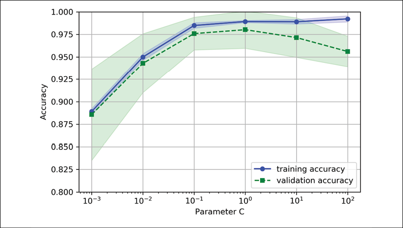
Similar to the learning_curve function, the validation_curve function uses stratified k-fold cross-validation by default to estimate the performance of the classifier. Inside the validation_curve function, we specified the parameter that we wanted to evaluate. In this case, it is C, the inverse regularization parameter of the LogisticRegression classifier, which we wrote as 'logisticregression__C' to access the LogisticRegression object inside the scikit-learn pipeline for a specified value range that we set via the param_range parameter. Similar to the learning curve example in the previous section, we plotted the average training and cross-validation accuracies and the corresponding standard deviations.

Although the differences in the accuracy for varying values of C are subtle, we can see that the model slightly underfits the data when we increase the regularization strength (small values of C). However, for large values of C, it means lowering the strength of regularization, so the model tends to slightly overfit the data. In this case, the sweet spot appears to be between 0.01 and 0.1 of the C value.

Fine-tuning machine learning models via grid search

In machine learning, we have two types of parameters: those that are learned from the training data, for example, the weights in logistic regression, and the parameters of a learning algorithm that are optimized separately. The latter are the tuning parameters (or hyperparameters) of a model, for example, the regularization parameter in logistic regression or the depth parameter of a decision tree.

In the previous section, we used validation curves to improve the performance of a model by tuning one of its hyperparameters. In this section, we will take a look at a popular hyperparameter optimization technique called grid search, which can further help to improve the performance of a model by finding the optimal combination of hyperparameter values.

Tuning hyperparameters via grid search

The grid search approach is quite simple: it's a brute-force exhaustive search paradigm where we specify a list of values for different hyperparameters, and the computer evaluates the model performance for each combination to obtain the optimal combination of values from this set:

>>> from sklearn.model_selection import GridSearchCV
>>> from sklearn.svm import SVC
>>> pipe_svc = make_pipeline(StandardScaler(),
...                          SVC(random_state=1))
>>> param_range = [0.0001, 0.001, 0.01, 0.1,
...                1.0, 10.0, 100.0, 1000.0]
>>> param_grid = [{'svc__C': param_range,
...                'svc__kernel': ['linear']},
...               {'svc__C': param_range,
...                'svc__gamma': param_range,
...                'svc__kernel': ['rbf']}]
>>> gs = GridSearchCV(estimator=pipe_svc,
...                   param_grid=param_grid,
...                   scoring='accuracy',
...                   cv=10,
...                   refit=True,
...                   n_jobs=-1)
>>> gs = gs.fit(X_train, y_train)
>>> print(gs.best_score_)
0.9846153846153847
>>> print(gs.best_params_)
{'svc__C': 100.0, 'svc__gamma': 0.001, 'svc__kernel': 'rbf'}

Using the preceding code, we initialized a GridSearchCV object from the sklearn.model_selection module to train and tune an SVM pipeline. We set the param_grid parameter of GridSearchCV to a list of dictionaries to specify the parameters that we'd want to tune. For the linear SVM, we only evaluated the inverse regularization parameter, C; for the RBF kernel SVM, we tuned both the svc__C and svc__gamma parameters. Note that the svc__gamma parameter is specific to kernel SVMs.

After we used the training data to perform the grid search, we obtained the score of the best-performing model via the best_score_ attribute and looked at its parameters, which can be accessed via the best_params_ attribute. In this particular case, the RBF kernel SVM model with svc__C = 100.0 yielded the best k-fold cross-validation accuracy: 98.5 percent.

Finally, we use the independent test dataset to estimate the performance of the best-selected model, which is available via the best_estimator_ attribute of the GridSearchCV object:

>>> clf = gs.best_estimator_
>>> clf.fit(X_train, y_train)
>>> print('Test accuracy: %.3f' % clf.score(X_test, y_test))
Test accuracy: 0.974

Please note that fitting a model with the best settings (gs.best_estimator_) on the training set manually via clf.fit(X_train, y_train) after completing the grid search is not necessary. The GridSearchCV class has a refit parameter, which will refit the gs.best_estimator_ to the whole training set automatically if we set refit=True (default).

Algorithm selection with nested cross-validation

Using k-fold cross-validation in combination with grid search is a useful approach for fine-tuning the performance of a machine learning model by varying its hyperparameter values, as we saw in the previous subsection. If we want to select among different machine learning algorithms, though, another recommended approach is nested cross-validation. In a nice study on the bias in error estimation, Sudhir Varma and Richard Simon concluded that the true error of the estimate is almost unbiased relative to the test dataset when nested cross-validation is used (Bias in Error Estimation When Using Cross-Validation for Model Selection, BMC Bioinformatics, S. Varma and R. Simon, 7(1): 91, 2006).

In nested cross-validation, we have an outer k-fold cross-validation loop to split the data into training and test folds, and an inner loop is used to select the model using k-fold cross-validation on the training fold. After model selection, the test fold is then used to evaluate the model performance. The following figure explains the concept of nested cross-validation with only five outer and two inner folds, which can be useful for large datasets where computational performance is important; this particular type of nested cross-validation is also known as 5x2 cross-validation:

In scikit-learn, we can perform nested cross-validation as follows:

>>> gs = GridSearchCV(estimator=pipe_svc,
...                   param_grid=param_grid,
...                   scoring='accuracy',
...                   cv=2)
>>> scores = cross_val_score(gs, X_train, y_train,
...                          scoring='accuracy', cv=5)
>>> print('CV accuracy: %.3f +/- %.3f' % (np.mean(scores),
...                                       np.std(scores)))
CV accuracy: 0.974 +/- 0.015

The returned average cross-validation accuracy gives us a good estimate of what to expect if we tune the hyperparameters of a model and use it on unseen data.

For example, we can use the nested cross-validation approach to compare an SVM model to a simple decision tree classifier; for simplicity, we will only tune its depth parameter:

>>> from sklearn.tree import DecisionTreeClassifier
>>> gs = GridSearchCV(estimator=DecisionTreeClassifier(
...                       random_state=0),
...                   param_grid=[{'max_depth': [1, 2, 3,
...                                              4, 5, 6,
...                                              7, None]}],
...                   scoring='accuracy',
...                   cv=2)
>>> scores = cross_val_score(gs, X_train, y_train,
...                          scoring='accuracy', cv=5)
>>> print('CV accuracy: %.3f +/- %.3f' % (np.mean(scores),
...                                       np.std(scores)))
CV accuracy: 0.934 +/- 0.016

As we can see, the nested cross-validation performance of the SVM model (97.4 percent) is notably better than the performance of the decision tree (93.4 percent), and thus, we'd expect that it might be the better choice to classify new data that comes from the same population as this particular dataset.

Looking at different performance evaluation metrics

In the previous sections and chapters, we evaluated different machine learning models using the prediction accuracy, which is a useful metric with which to quantify the performance of a model in general. However, there are several other performance metrics that can be used to measure a model's relevance, such as precision, recall, and the F1 score.

Reading a confusion matrix

Before we get into the details of different scoring metrics, let's take a look at a confusion matrix, a matrix that lays out the performance of a learning algorithm.

A confusion matrix is simply a square matrix that reports the counts of the true positive (TP), true negative (TN), false positive (FP), and false negative (FN) predictions of a classifier, as shown in the following figure:

Although these metrics can be easily computed manually by comparing the true and predicted class labels, scikit-learn provides a convenient confusion_matrix function that we can use, as follows:

>>> from sklearn.metrics import confusion_matrix
>>> pipe_svc.fit(X_train, y_train)
>>> y_pred = pipe_svc.predict(X_test)
>>> confmat = confusion_matrix(y_true=y_test, y_pred=y_pred)
>>> print(confmat)
[[71  1]
[ 2 40]]

The array that was returned after executing the code provides us with information about the different types of error the classifier made on the test dataset. We can map this information onto the confusion matrix illustration in the previous figure using Matplotlib's matshow function:

>>> fig, ax = plt.subplots(figsize=(2.5, 2.5))
>>> ax.matshow(confmat, cmap=plt.cm.Blues, alpha=0.3)
>>> for i in range(confmat.shape[0]):
...     for j in range(confmat.shape[1]):
...         ax.text(x=j, y=i,
...                 s=confmat[i, j],
...                 va='center', ha='center')
>>> plt.xlabel('Predicted label')
>>> plt.ylabel('True label')
>>> plt.show()

Now, the following confusion matrix plot, with the added labels, should make the results a little bit easier to interpret:

Assuming that class 1 (malignant) is the positive class in this example, our model correctly classified 71 of the examples that belong to class 0 (TN) and 40 examples that belong to class 1 (TP), respectively. However, our model also incorrectly misclassified two examples from class 1 as class 0 (FN), and it predicted that one example is malignant although it is a benign tumor (FP). In the next subsection, we will learn how we can use this information to calculate various error metrics.

Optimizing the precision and recall of a classification model

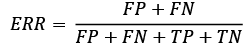
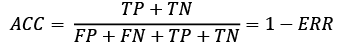
Both the prediction error (ERR) and accuracy (ACC) provide general information about how many examples are misclassified. The error can be understood as the sum of all false predictions divided by the number of total predictions, and the accuracy is calculated as the sum of correct predictions divided by the total number of predictions, respectively:

The prediction accuracy can then be calculated directly from the error:

The true positive rate (TPR) and false positive rate (FPR) are performance metrics that are especially useful for imbalanced class problems:

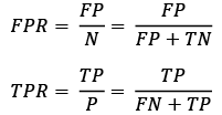
In tumor diagnosis, for example, we are more concerned about the detection of malignant tumors in order to help a patient with the appropriate treatment. However, it is also important to decrease the number of benign tumors incorrectly classified as malignant (FP) to not unnecessarily concern patients. In contrast to the FPR, the TPR provides useful information about the fraction of positive (or relevant) examples that were correctly identified out of the total pool of positives (P).

The performance metrics precision (PRE) and recall (REC) are related to those TP and TN rates, and in fact, REC is synonymous with TPR:

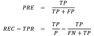
Revisiting the malignant tumor detection example, optimizing for recall helps with minimizing the chance of not detecting a malignant tumor. However, this comes at the cost of predicting malignant tumors in patients although the patients are healthy (a high number of FP). If we optimize for precision, on the other hand, we emphasize correctness if we predict that a patient has a malignant tumor. However, this comes at the cost of missing malignant tumors more frequently (a high number of FN).

To balance the up- and down-sides of optimizing PRE and REC, often a combination of PRE and REC is used, the so-called F1 score:

Those scoring metrics are all implemented in scikit-learn and can be imported from the sklearn.metrics module as shown in the following snippet:

>>> from sklearn.metrics import precision_score
>>> from sklearn.metrics import recall_score, f1_score
>>> print('Precision: %.3f' % precision_score(
...           y_true=y_test, y_pred=y_pred))
Precision: 0.976
>>> print('Recall: %.3f' % recall_score(
...           y_true=y_test, y_pred=y_pred))
Recall: 0.952
>>> print('F1: %.3f' % f1_score(
...           y_true=y_test, y_pred=y_pred))
F1: 0.964

Furthermore, we can use a different scoring metric than accuracy in the GridSearchCV via the scoring parameter. A complete list of the different values that are accepted by the scoring parameter can be found at http://scikit-learn.org/stable/modules/model_evaluation.html.

Remember that the positive class in scikit-learn is the class that is labeled as class 1. If we want to specify a different positive label, we can construct our own scorer via the make_scorer function, which we can then directly provide as an argument to the scoring parameter in GridSearchCV (in this example, using the f1_score as a metric):

>>> from sklearn.metrics import make_scorer, f1_score
>>> c_gamma_range = [0.01, 0.1, 1.0, 10.0]
>>> param_grid = [{'svc__C': c_gamma_range,
...                'svc__kernel': ['linear']},
...               {'svc__C': c_gamma_range,
...                'svc__gamma': c_gamma_range,
...                'svc__kernel': ['rbf']}]
>>> scorer = make_scorer(f1_score, pos_label=0)
>>> gs = GridSearchCV(estimator=pipe_svc,
...                   param_grid=param_grid,
...                   scoring=scorer,
...                   cv=10)
>>> gs = gs.fit(X_train, y_train)
>>> print(gs.best_score_)
0.986202145696
>>> print(gs.best_params_)
{'svc__C': 10.0, 'svc__gamma': 0.01, 'svc__kernel': 'rbf'}

Plotting a receiver operating characteristic

Receiver operating characteristic (ROC) graphs are useful tools to select models for classification based on their performance with respect to the FPR and TPR, which are computed by shifting the decision threshold of the classifier. The diagonal of a ROC graph can be interpreted as random guessing, and classification models that fall below the diagonal are considered as worse than random guessing. A perfect classifier would fall into the top-left corner of the graph with a TPR of 1 and an FPR of 0. Based on the ROC curve, we can then compute the so-called ROC area under the curve (ROC AUC) to characterize the performance of a classification model.

Similar to ROC curves, we can compute precision-recall curves for different probability thresholds of a classifier. A function for plotting those precision-recall curves is also implemented in scikit-learn and is documented at http://scikit-learn.org/stable/modules/generated/sklearn.metrics.precision_recall_curve.html.

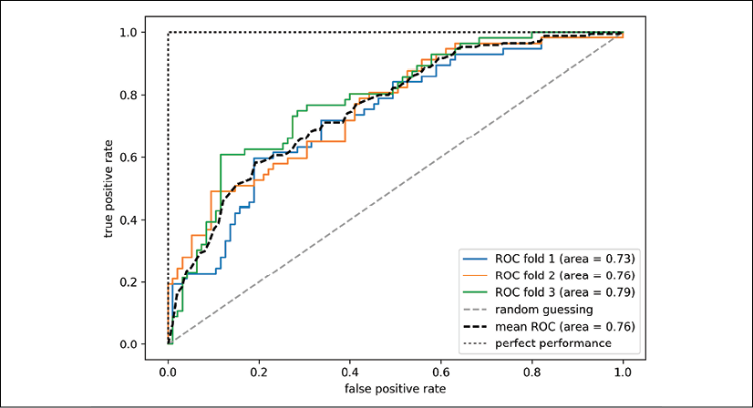
Executing the following code example, we will plot a ROC curve of a classifier that only uses two features from the Breast Cancer Wisconsin dataset to predict whether a tumor is benign or malignant. Although we are going to use the same logistic regression pipeline that we defined previously, we are only using two features this time. This is to make the classification task more challenging for the classifier, by witholding useful information contained in the other features, so that the resulting ROC curve becomes visually more interesting. For similar reasons, we are also reducing the number of folds in the StratifiedKFold validator to three. The code is as follows:

>>> from sklearn.metrics import roc_curve, auc
>>> from scipy import interp
>>> pipe_lr = make_pipeline(StandardScaler(),
...                         PCA(n_components=2),
...                         LogisticRegression(penalty='l2',
...                                            random_state=1,
...                                            solver='lbfgs',
...                                            C=100.0))
>>> X_train2 = X_train[:, [4, 14]]
>>> cv = list(StratifiedKFold(n_splits=3,
...                           random_state=1).split(X_train,
...                                                 y_train))
>>> fig = plt.figure(figsize=(7, 5))
>>> mean_tpr = 0.0
>>> mean_fpr = np.linspace(0, 1, 100)
>>> all_tpr = []
>>> for i, (train, test) in enumerate(cv):
...     probas = pipe_lr.fit(
...         X_train2[train],
...         y_train[train]).predict_proba(X_train2[test])
...     fpr, tpr, thresholds = roc_curve(y_train[test],
...                                      probas[:, 1],
...                                      pos_label=1)
...     mean_tpr += interp(mean_fpr, fpr, tpr)
...     mean_tpr[0] = 0.0
...     roc_auc = auc(fpr, tpr)
...     plt.plot(fpr,
...              tpr,
...              label='ROC fold %d (area = %0.2f)'
...              % (i+1, roc_auc))
>>> plt.plot([0, 1],
...          [0, 1],
...          linestyle='--',
...          color=(0.6, 0.6, 0.6),
...          label='Random guessing')
>>> mean_tpr /= len(cv)
>>> mean_tpr[-1] = 1.0
>>> mean_auc = auc(mean_fpr, mean_tpr)
>>> plt.plot(mean_fpr, mean_tpr, 'k--',
...          label='Mean ROC (area = %0.2f)' % mean_auc, lw=2)
>>> plt.plot([0, 0, 1],
...          [0, 1, 1],
...          linestyle=':',
...          color='black',
...          label='Perfect performance')
>>> plt.xlim([-0.05, 1.05])
>>> plt.ylim([-0.05, 1.05])
>>> plt.xlabel('False positive rate')
>>> plt.ylabel('True positive rate')
>>> plt.legend(loc="lower right")
>>> plt.show()

In the preceding code example, we used the already familiar StratifiedKFold class from scikit-learn and calculated the ROC performance of the LogisticRegression classifier in our pipe_lr pipeline using the roc_curve function from the sklearn.metrics module separately for each iteration. Furthermore, we interpolated the average ROC curve from the three folds via the interp function that we imported from SciPy and calculated the area under the curve via the auc function. The resulting ROC curve indicates that there is a certain degree of variance between the different folds, and the average ROC AUC (0.76) falls between a perfect score (1.0) and random guessing (0.5):

Note that if we are just interested in the ROC AUC score, we could also directly import the roc_auc_score function from the sklearn.metrics submodule, which can be used similarly to the other scoring functions (for example, precision_score) that were introduced in the previous sections.

Reporting the performance of a classifier as the ROC AUC can yield further insights into a classifier's performance with respect to imbalanced samples. However, while the accuracy score can be interpreted as a single cut-off point on an ROC curve, A. P. Bradley showed that the ROC AUC and accuracy metrics mostly agree with each other: The use of the area under the ROC curve in the evaluation of machine learning algorithms, A. P. Bradley, Pattern Recognition, 30(7): 1145-1159, 1997.

Scoring metrics for multiclass classification

The scoring metrics that we've discussed so far are specific to binary classification systems. However, scikit-learn also implements macro and micro averaging methods to extend those scoring metrics to multiclass problems via one-vs.-all (OvA) classification. The micro-average is calculated from the individual TPs, TNs, FPs, and FNs of the system. For example, the micro-average of the precision score in a k-class system can be calculated as follows:

The macro-average is simply calculated as the average scores of the different systems:

Micro-averaging is useful if we want to weight each instance or prediction equally, whereas macro-averaging weights all classes equally to evaluate the overall performance of a classifier with regard to the most frequent class labels.

If we are using binary performance metrics to evaluate multiclass classification models in scikit-learn, a normalized or weighted variant of the macro-average is used by default. The weighted macro-average is calculated by weighting the score of each class label by the number of true instances when calculating the average. The weighted macro-average is useful if we are dealing with class imbalances, that is, different numbers of instances for each label.

While the weighted macro-average is the default for multiclass problems in scikit-learn, we can specify the averaging method via the average parameter inside the different scoring functions that we import from the sklearn.metrics module, for example, the precision_score or make_scorer functions:

>>> pre_scorer = make_scorer(score_func=precision_score,
...                          pos_label=1,
...                          greater_is_better=True,
...                          average='micro')

Dealing with class imbalance

We've mentioned class imbalances several times throughout this chapter, and yet we haven't actually discussed how to deal with such scenarios appropriately if they occur. Class imbalance is a quite common problem when working with real-world data—examples from one class or multiple classes are over-represented in a dataset. We can think of several domains where this may occur, such as spam filtering, fraud detection, or screening for diseases.

Imagine that the Breast Cancer Wisconsin dataset that we've been working with in this chapter consisted of 90 percent healthy patients. In this case, we could achieve 90 percent accuracy on the test dataset by just predicting the majority class (benign tumor) for all examples, without the help of a supervised machine learning algorithm. Thus, training a model on such a dataset that achieves approximately 90 percent test accuracy would mean our model hasn't learned anything useful from the features provided in this dataset.

In this section, we will briefly go over some of the techniques that could help with imbalanced datasets. But before we discuss different methods to approach this problem, let's create an imbalanced dataset from our dataset, which originally consisted of 357 benign tumors (class 0) and 212 malignant tumors (class 1):

>>> X_imb = np.vstack((X[y == 0], X[y == 1][:40]))
>>> y_imb = np.hstack((y[y == 0], y[y == 1][:40]))

In this code snippet, we took all 357 benign tumor examples and stacked them with the first 40 malignant examples to create a stark class imbalance. If we were to compute the accuracy of a model that always predicts the majority class (benign, class 0), we would achieve a prediction accuracy of approximately 90 percent:

>>> y_pred = np.zeros(y_imb.shape[0])
>>> np.mean(y_pred == y_imb) * 100
89.92443324937027

Thus, when we fit classifiers on such datasets, it would make sense to focus on other metrics than accuracy when comparing different models, such as precision, recall, the ROC curve—whatever we care most about in our application. For instance, our priority might be to identify the majority of patients with malignant cancer to recommend an additional screening, so recall should be our metric of choice. In spam filtering, where we don't want to label emails as spam if the system is not very certain, precision might be a more appropriate metric.

Aside from evaluating machine learning models, class imbalance influences a learning algorithm during model fitting itself. Since machine learning algorithms typically optimize a reward or cost function that is computed as a sum over the training examples that it sees during fitting, the decision rule is likely going to be biased toward the majority class.

In other words, the algorithm implicitly learns a model that optimizes the predictions based on the most abundant class in the dataset, in order to minimize the cost or maximize the reward during training.

One way to deal with imbalanced class proportions during model fitting is to assign a larger penalty to wrong predictions on the minority class. Via scikit-learn, adjusting such a penalty is as convenient as setting the class_weight parameter to class_weight='balanced', which is implemented for most classifiers.

Other popular strategies for dealing with class imbalance include upsampling the minority class, downsampling the majority class, and the generation of synthetic training examples. Unfortunately, there's no universally best solution or technique that works best across different problem domains. Thus, in practice, it is recommended to try out different strategies on a given problem, evaluate the results, and choose the technique that seems most appropriate.

The scikit-learn library implements a simple resample function that can help with the upsampling of the minority class by drawing new samples from the dataset with replacement. The following code will take the minority class from our imbalanced Breast Cancer Wisconsin dataset (here, class 1) and repeatedly draw new samples from it until it contains the same number of examples as class label 0:

>>> from sklearn.utils import resample
>>> print('Number of class 1 examples before:',
...       X_imb[y_imb == 1].shape[0])
Number of class 1 examples before: 40
>>> X_upsampled, y_upsampled = resample(
...         X_imb[y_imb == 1],
...         y_imb[y_imb == 1],
...         replace=True,
...         n_samples=X_imb[y_imb == 0].shape[0],
...         random_state=123)
>>> print('Number of class 1 examples after:',
...       X_upsampled.shape[0])
Number of class 1 examples after: 357

After resampling, we can then stack the original class 0 samples with the upsampled class 1 subset to obtain a balanced dataset as follows:

>>> X_bal = np.vstack((X[y == 0], X_upsampled))
>>> y_bal = np.hstack((y[y == 0], y_upsampled))

Consequently, a majority vote prediction rule would only achieve 50 percent accuracy:

>>> y_pred = np.zeros(y_bal.shape[0])
>>> np.mean(y_pred == y_bal) * 100
50

Similarly, we could downsample the majority class by removing training examples from the dataset. To perform downsampling using the resample function, we could simply swap the class 1 label with class 0 in the previous code example and vice versa.

Summary

At the beginning of this chapter, we discussed how to chain different transformation techniques and classifiers in convenient model pipelines that help us to train and evaluate machine learning models more efficiently. We then used those pipelines to perform k-fold cross-validation, one of the essential techniques for model selection and evaluation. Using k-fold cross-validation, we plotted learning and validation curves to diagnose common problems of learning algorithms, such as overfitting and underfitting.

Using grid search, we further fine-tuned our model. We then used confusion matrices and various performance metrics to evaluate and optimize a model's performance for specific problem tasks. Finally, we concluded this chapter by discussing different methods for dealing with imbalanced data, which is a common problem in many real-world applications. Now, you should be well-equipped with the essential techniques to build supervised machine learning models for classification successfully.

In the next chapter, we will look at ensemble methods: methods that allow us to combine multiple models and classification algorithms to boost the predictive performance of a machine learning system even further.