In the previous chapter, we focused on recurrent neural networks for modeling sequences. In this chapter, we will explore generative adversarial networks (GANs) and see their application in synthesizing new data samples. GANs are considered to be the most important breakthrough in deep learning, allowing computers to generate new data (such as new images).
In this chapter, we will cover the following topics:
- Introducing generative models for synthesizing new data
- Autoencoders, variational autoencoders (VAEs), and their relationship to GANs
- Understanding the building blocks of GANs
- Implementing a simple GAN model to generate handwritten digits
- Understanding transposed convolution and batch normalization (BatchNorm or BN)
- Improving GANs: deep convolutional GANs and GANs using the Wasserstein distance
Introducing generative adversarial networks
Let's first look at the foundations of GAN models. The overall objective of a GAN is to synthesize new data that has the same distribution as its training dataset. Therefore, GANs, in their original form, are considered to be in the unsupervised learning category of machine learning tasks, since no labeled data is required. It is worth noting, however, that extensions made to the original GAN can lie in both semi-supervised and supervised tasks.
The general GAN concept was first proposed in 2014 by Ian Goodfellow and his colleagues as a method for synthesizing new images using deep neural networks (NNs) (Goodfellow, I., Pouget-Abadie, J., Mirza, M., Xu, B., Warde-Farley, D., Ozair, S., Courville, A. and Bengio, Y., Generative Adversarial Nets, in Advances in Neural Information Processing Systems, pp. 2672-2680, 2014). While the initial GAN architecture proposed in this paper was based on fully connected layers, similar to multilayer perceptron architectures, and trained to generate low-resolution MNIST-like handwritten digits, it served more as a proof of concept to demonstrate the feasibility of this new approach.
However, since its introduction, the original authors, as well as many other researchers, have proposed numerous improvements and various applications in different fields of engineering and science; for example, in computer vision, GANs are used for image-to-image translation (learning how to map an input image to an output image), image super-resolution (making a high-resolution image from a low-resolution version), image inpainting (learning how to reconstruct the missing parts of an image), and many more applications. For instance, recent advances in GAN research have led to models that are able to generate new, high-resolution face images. Examples of such high-resolution images can be found on https://www.thispersondoesnotexist.com/, which showcases synthetic face images generated by a GAN.
Starting with autoencoders
Before we discuss how GANs work, we will first start with autoencoders, which can compress and decompress training data. While standard autoencoders cannot generate new data, understanding their function will help you to navigate GANs in the next section.
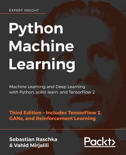
Autoencoders are composed of two networks concatenated together: an encoder network and a decoder network. The encoder network receives a d-dimensional input feature vector associated with example x (that is, ![]() ) and encodes it into a p-dimensional vector, z (that is,
) and encodes it into a p-dimensional vector, z (that is, ![]() ). In other words, the role of the encoder is to learn how to model the function
). In other words, the role of the encoder is to learn how to model the function ![]() . The encoded vector, z, is also called the latent vector, or the latent feature representation. Typically, the dimensionality of the latent vector is less than that of the input examples; in other words, p < d. Hence, we can say that the encoder acts as a data compression function. Then, the decoder decompresses
. The encoded vector, z, is also called the latent vector, or the latent feature representation. Typically, the dimensionality of the latent vector is less than that of the input examples; in other words, p < d. Hence, we can say that the encoder acts as a data compression function. Then, the decoder decompresses ![]() from the lower-dimensional latent vector, z, where we can think of the decoder as a function,
from the lower-dimensional latent vector, z, where we can think of the decoder as a function, ![]() . A simple autoencoder architecture is shown in the following figure, where the encoder and decoder parts consist of only one fully connected layer each:
. A simple autoencoder architecture is shown in the following figure, where the encoder and decoder parts consist of only one fully connected layer each:
The connection between autoencoders and dimensionality reduction
In Chapter 5, Compressing Data via Dimensionality Reduction, you learned about dimensionality reduction techniques, such as principal component analysis (PCA) and linear discriminant analysis (LDA). Autoencoders can be used as a dimensionality reduction technique as well. In fact, when there is no nonlinearity in either of the two subnetworks (encoder and decoder), then the autoencoder approach is almost identical to PCA.
In this case, if we assume the weights of a single-layer encoder (no hidden layer and no nonlinear activation function) are denoted by the matrix U, then the encoder models ![]() . Similarly, a single-layer linear decoder models
. Similarly, a single-layer linear decoder models ![]() . Putting these two components together, we have
. Putting these two components together, we have ![]() . This is exactly what PCA does, with the exception that PCA has an additional orthonormal constraint:
. This is exactly what PCA does, with the exception that PCA has an additional orthonormal constraint: ![]() .
.
While the previous figure depicts an autoencoder without hidden layers within the encoder and decoder, we can, of course, add multiple hidden layers with nonlinearities (as in a multilayer NN) to construct a deep autoencoder that can learn more effective data compression and reconstruction functions. Also, note that the autoencoder mentioned in this section uses fully connected layers. When we work with images, however, we can replace the fully connected layers with convolutional layers, as you learned in Chapter 15, Classifying Images with Deep Convolutional Neural Networks.
Other types of autoencoders based on the size of latent space
As previously mentioned, the dimensionality of an autoencoder's latent space is typically lower than the dimensionality of the inputs (p < d), which makes autoencoders suitable for dimensionality reduction. For this reason, the latent vector is also often referred to as the "bottleneck," and this particular configuration of an autoencoder is also called undercomplete. However, there is a different category of autoencoders, called overcomplete, where the dimensionality of the latent vector, z, is, in fact, greater than the dimensionality of the input examples (p > d).
When training an overcomplete autoencoder, there is a trivial solution where the encoder and the decoder can simply learn to copy (memorize) the input features to their output layer. Obviously, this solution is not very useful. However, with some modifications to the training procedure, overcomplete autoencoders can be used for noise reduction.
In this case, during training, random noise, ![]() , is added to the input examples and the network learns to reconstruct the clean example, x, from the noisy signal,
, is added to the input examples and the network learns to reconstruct the clean example, x, from the noisy signal, ![]() . Then, at evaluation time, we provide the new examples that are naturally noisy (that is, noise is already present such that no additional artificial noise,
. Then, at evaluation time, we provide the new examples that are naturally noisy (that is, noise is already present such that no additional artificial noise, ![]() , is added) in order to remove the existing noise from these examples. This particular autoencoder architecture and training method is referred to as a denoising autoencoder.
, is added) in order to remove the existing noise from these examples. This particular autoencoder architecture and training method is referred to as a denoising autoencoder.
If you are interested, you can learn more about it in the research article Stacked denoising autoencoders: Learning useful representations in a deep network with a local denoising criterion by Vincent et al., which is freely available at http://www.jmlr.org/papers/v11/vincent10a.html.
Generative models for synthesizing new data
Autoencoders are deterministic models, which means that after an autoencoder is trained, given an input, x, it will be able to reconstruct the input from its compressed version in a lower-dimensional space. Therefore, it cannot generate new data beyond reconstructing its input through the transformation of the compressed representation.
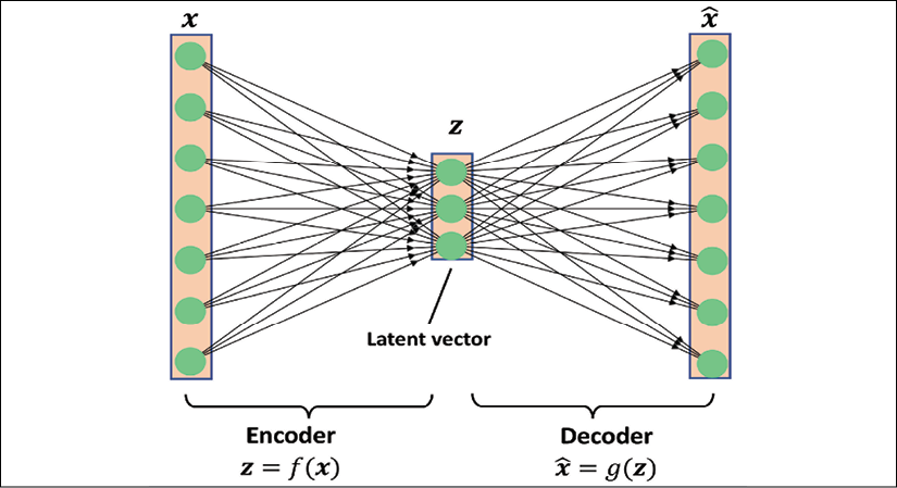
A generative model, on the other hand, can generate a new example, ![]() , from a random vector, z (corresponding to the latent representation). A schematic representation of a generative model is shown in the following figure. The random vector, z, comes from a simple distribution with fully known characteristics, so we can easily sample from such a distribution. For example, each element of z may come from the uniform distribution in the range [–1, 1] (for which we write
, from a random vector, z (corresponding to the latent representation). A schematic representation of a generative model is shown in the following figure. The random vector, z, comes from a simple distribution with fully known characteristics, so we can easily sample from such a distribution. For example, each element of z may come from the uniform distribution in the range [–1, 1] (for which we write ![]() ) or from a standard normal distribution (in which case, we write
) or from a standard normal distribution (in which case, we write ![]() ).
).
As we have shifted our attention from autoencoders to generative models, you may have noticed that the decoder component of an autoencoder has some similarities with a generative model. In particular, they both receive a latent vector, z, as input and return an output in the same space as x. (For the autoencoder, ![]() is the reconstruction of an input, x, and for the generative model,
is the reconstruction of an input, x, and for the generative model, ![]() is a synthesized sample.)
is a synthesized sample.)
However, the major difference between the two is that we do not know the distribution of z in the autoencoder, while in a generative model, the distribution of z is fully characterizable. It is possible to generalize an autoencoder into a generative model, though. One approach is VAEs.
In a VAE receiving an input example, x, the encoder network is modified in such a way that it computes two moments of the distribution of the latent vector: the mean, ![]() , and variance,
, and variance, ![]() . During the training of a VAE, the network is forced to match these moments with those of a standard normal distribution (that is, zero mean and unit variance). Then, after the VAE model is trained, the encoder is discarded, and we can use the decoder network to generate new examples,
. During the training of a VAE, the network is forced to match these moments with those of a standard normal distribution (that is, zero mean and unit variance). Then, after the VAE model is trained, the encoder is discarded, and we can use the decoder network to generate new examples, ![]() , by feeding random z vectors from the "learned" Gaussian distribution.
, by feeding random z vectors from the "learned" Gaussian distribution.
Besides VAEs, there are other types of generative models, for example, autoregressive models and normalizing flow models. However, in this chapter, we are only going to focus on GAN models, which are among the most recent and most popular types of generative models in deep learning.
What is a generative model?
Note that generative models are traditionally defined as algorithms that model data input distributions, p(x), or the joint distributions of the input data and associated targets, p(x, y). By definition, these models are also capable of sampling from some feature, ![]() , conditioned on another feature,
, conditioned on another feature, ![]() , which is known as conditional inference. In the context of deep learning, however, the term generative model is typically used to refer to models that generate realistic-looking data. This means that we can sample from input distributions, p(x), but we are not necessarily able to perform conditional inference.
, which is known as conditional inference. In the context of deep learning, however, the term generative model is typically used to refer to models that generate realistic-looking data. This means that we can sample from input distributions, p(x), but we are not necessarily able to perform conditional inference.
Generating new samples with GANs
To understand what GANs do in a nutshell, let's first assume we have a network that receives a random vector, z, sampled from a known distribution and generates an output image, x. We will call this network generator (G) and use the notation ![]() to refer to the generated output. Assume our goal is to generate some images, for example, face images, images of buildings, images of animals, or even handwritten digits such as MNIST.
to refer to the generated output. Assume our goal is to generate some images, for example, face images, images of buildings, images of animals, or even handwritten digits such as MNIST.
As always, we will initialize this network with random weights. Therefore, the first output images, before these weights are adjusted, will look like white noise. Now, imagine there is a function that can assess the quality of images (let's call it an assessor function).
If such a function exists, we can use the feedback from that function to tell our generator network how to adjust its weights in order to improve the quality of the generated images. This way, we can train the generator based on the feedback from that assessor function, such that the generator learns to improve its output toward producing realistic-looking images.
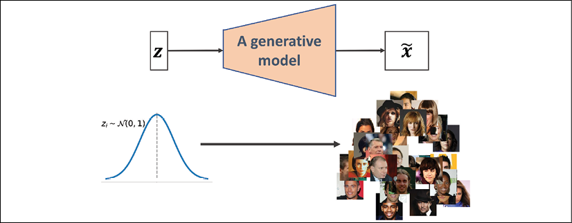
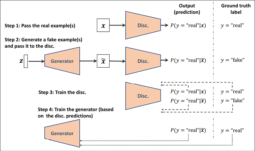
While an assessor function, as described in the previous paragraph, would make the image generation task very easy, the question is whether such a universal function to assess the quality of images exists and, if so, how it is defined. Obviously, as humans, we can easily assess the quality of output images when we observe the outputs of the network; although, we cannot (yet) backpropagate the result from our brain to the network. Now, if our brain can assess the quality of synthesized images, can we design an NN model to do the same thing? In fact, that's the general idea of a GAN. As shown in the following figure, a GAN model consists of an additional NN called discriminator (D), which is a classifier that learns to detect a synthesized image, ![]() , from a real image, x:
, from a real image, x:
In a GAN model, the two networks, generator and discriminator, are trained together. At first, after initializing the model weights, the generator creates images that do not look realistic. Similarly, the discriminator does a poor job of distinguishing between real images and images synthesized by the generator. But over time (that is, through training), both networks become better as they interact with each other. In fact, the two networks play an adversarial game, where the generator learns to improve its output to be able to fool the discriminator. At the same time, the discriminator becomes better at detecting the synthesized images.
Understanding the loss functions of the generator and discriminator networks in a GAN model
The objective function of GANs, as described in the original paper Generative Adversarial Nets by Goodfellow et al. (https://papers.nips.cc/paper/5423-generative-adversarial-nets.pdf), is as follows:

Here, ![]() is called the value function, which can be interpreted as a payoff: we want to maximize its value with respect to the discriminator (D), while minimizing its value with respect to the generator (G), that is,
is called the value function, which can be interpreted as a payoff: we want to maximize its value with respect to the discriminator (D), while minimizing its value with respect to the generator (G), that is, ![]() . D(x) is the probability that indicates whether the input example, x, is real or fake (that is, generated). The expression
. D(x) is the probability that indicates whether the input example, x, is real or fake (that is, generated). The expression ![]() refers to the expected value of the quantity in brackets with respect to the examples from the data distribution (distribution of the real examples);
refers to the expected value of the quantity in brackets with respect to the examples from the data distribution (distribution of the real examples); ![]() refers to the expected value of the quantity with respect to the distribution of the input, z, vectors.
refers to the expected value of the quantity with respect to the distribution of the input, z, vectors.
One training step of a GAN model with such a value function requires two optimization steps: (1) maximizing the payoff for the discriminator and (2) minimizing the payoff for the generator. A practical way of training GANs is to alternate between these two optimization steps: (1) fix (freeze) the parameters of one network and optimize the weights of the other one, and (2) fix the second network and optimize the first one. This process should be repeated at each training iteration. Let's assume that the generator network is fixed, and we want to optimize the discriminator. Both terms in the value function ![]() contribute to optimizing the discriminator, where the first term corresponds to the loss associated with the real examples, and the second term is the loss for the fake examples. Therefore, when G is fixed, our objective is to maximize
contribute to optimizing the discriminator, where the first term corresponds to the loss associated with the real examples, and the second term is the loss for the fake examples. Therefore, when G is fixed, our objective is to maximize ![]() , which means making the discriminator better at distinguishing between real and generated images.
, which means making the discriminator better at distinguishing between real and generated images.
After optimizing the discriminator using the loss terms for real and fake samples, we then fix the discriminator and optimize the generator. In this case, only the second term in ![]() contributes to the gradients of the generator. As a result, when D is fixed, our objective is to minimize
contributes to the gradients of the generator. As a result, when D is fixed, our objective is to minimize ![]() , which can be written as
, which can be written as ![]() . As was mentioned in the original GAN paper by Goodfellow et al., this function,
. As was mentioned in the original GAN paper by Goodfellow et al., this function, ![]() , suffers from vanishing gradients in the early training stages. The reason for this is that the outputs, G(z), early in the learning process, look nothing like real examples, and therefore D(G(z)) will be close to zero with high confidence. This phenomenon is called saturation. To resolve this issue, we can reformulate the minimization objective,
, suffers from vanishing gradients in the early training stages. The reason for this is that the outputs, G(z), early in the learning process, look nothing like real examples, and therefore D(G(z)) will be close to zero with high confidence. This phenomenon is called saturation. To resolve this issue, we can reformulate the minimization objective, ![]() , by rewriting it as
, by rewriting it as ![]() .
.
This replacement means that for training the generator, we can swap the labels of real and fake examples and carry out a regular function minimization. In other words, even though the examples synthesized by the generator are fake and are therefore labeled 0, we can flip the labels by assigning label 1 to these examples, and minimize the binary cross-entropy loss with these new labels instead of maximizing ![]() .
.
Now that we have covered the general optimization procedure for training GAN models, let's explore the various data labels that we can use when training GANs. Given that the discriminator is a binary classifier (the class labels are 0 and 1 for fake and real images, respectively), we can use the binary cross-entropy loss function. Therefore, we can determine the ground truth labels for the discriminator loss as follows:
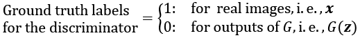
What about the labels to train the generator? As we want the generator to synthesize realistic images, we want to penalize the generator when its outputs are not classified as real by the discriminator. This means that we will assume the ground truth labels for the outputs of the generator to be 1 when computing the loss function for the generator.
Putting all of this together, the following figure displays the individual steps in a simple GAN model:
In the following section, we will implement a GAN from scratch to generate new handwritten digits.
Implementing a GAN from scratch
In this section, we will cover how to implement and train a GAN model to generate new images such as MNIST digits. Since the training on a normal central processing unit (CPU) may take a long time, in the following subsection, we will cover how to set up the Google Colab environment, which will allow us to run the computations on graphics processing units (GPUs).
Training GAN models on Google Colab
Some of the code examples in this chapter may require extensive computational resources that go beyond a commercial laptop or a workstation without a GPU. If you already have an NVIDIA GPU-enabled computing machine available, with CUDA and cuDNN libraries installed, you can use that to speed up the computations.
However, since many of us do not have access to high-performance computing resources, we will use the Google Colaboratory environment (often referred to as Google Colab), which is a free cloud computing service (available in most countries).
Google Colab provides Jupyter Notebook instances that run on the cloud; the notebooks can be saved on Google Drive or GitHub. While the platform provides various different computing resources, such as CPUs, GPUs, and even tensor processing units (TPUs), it is important to highlight that the execution time is currently limited to 12 hours. Therefore, any notebook running longer than 12 hours will be interrupted.
The code blocks in this chapter will need a maximum computing time of two to three hours, so this will not be an issue. However, if you decide to use Google Colab for other projects that take longer than 12 hours, be sure to use checkpointing and save intermediate checkpoints.
Jupyter Notebook
Jupyter Notebook is a graphical user interface (GUI) for running code interactively and interleaving it with text documentation and figures. Due to its versatility and ease of use, it has become one of the most popular tools in data science.
For more information about the general Jupyter Notebook GUI, please view the official documentation at https://jupyter-notebook.readthedocs.io/en/stable/. All the code in this book is also available in the form of Jupyter notebooks, and a short introduction can be found in the code directory of the first chapter at https://github.com/rasbt/python-machine-learning-book-3rd-edition/tree/master/ch01#pythonjupyter-notebook.
Lastly, we highly recommend Adam Rule et al.'s article Ten simple rules for writing and sharing computational analyses in Jupyter Notebooks on using Jupyter Notebook effectively in scientific research projects, which is freely available at https://journals.plos.org/ploscompbiol/article?id=10.1371/journal.pcbi.1007007.
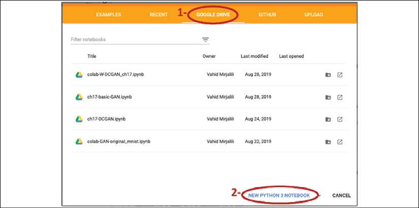
Accessing Google Colab is very straightforward. You can visit https://colab.research.google.com, which automatically takes you to a prompt window where you can see your existing Jupyter notebooks. From this prompt window, click the GOOGLE DRIVE tab, as shown in the following figure. This is where you will save the notebook on your Google Drive.
Then, to create a new notebook, click on the link NEW PYTHON 3 NOTEBOOK at the bottom of the prompt window:
This will create and open a new notebook for you. All the code examples you write in this notebook will be automatically saved, and you can later access the notebook from your Google Drive in a directory called Colab Notebooks.
In the next step, we want to utilize GPUs to run the code examples in this notebook. To do this, from the Runtime option in the menu bar of this notebook, click on Change runtime type and select GPU, as shown in the following figure:

In the last step, we just need to install the Python packages that we will need for this chapter. The Colab Notebooks environment already comes with certain packages, such as NumPy, SciPy, and the latest stable version of TensorFlow. However, at the time of writing, the latest stable version on Google Colab is TensorFlow 1.15.0, but we want to use TensorFlow 2.0. Therefore, first we need to install TensorFlow 2.0 with GPU support by executing the following command in a new cell of this notebook:
! pip install -q tensorflow-gpu==2.0.0
(In a Jupyter notebook, a cell starting with an exclamation mark will be interpreted as a Linux shell command.)
Now, we can test the installation and verify that the GPU is available using the following code:
>>> import tensorflow as tf
>>> print(tf.__version__)
'2.0.0'
>>> print("GPU Available:", tf.test.is_gpu_available())
GPU Available: True
>>> if tf.test.is_gpu_available():
...     device_name = tf.test.gpu_device_name()
... else:
...     device_name = '/CPU:0'
>>> print(device_name)
'/device:GPU:0'
Furthermore, if you want to save the model to your personal Google Drive, or transfer or upload other files, you need to mount the Google Drive. To do this, execute the following in a new cell of the notebook:
>>> from google.colab import drive
>>> drive.mount('/content/drive/')
This will provide a link to authenticate the Colab Notebook accessing your Google Drive. After following the instructions for authentication, it will provide an authentication code that you need to copy and paste into the designated input field below the cell you have just executed. Then, your Google Drive will be mounted and available at /content/drive/My Drive.
Implementing the generator and the discriminator networks
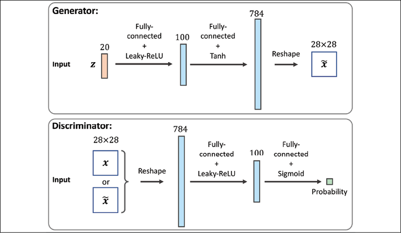
We will start the implementation of our first GAN model with a generator and a discriminator as two fully connected networks with one or more hidden layers (see the following figure).
This is the original GAN version, which we will refer to as vanilla GAN.
In this model, for each hidden layer, we will apply the leaky ReLU activation function. The use of ReLU results in sparse gradients, which may not be suitable when we want to have the gradients for the full range of input values. In the discriminator network, each hidden layer is also followed by a dropout layer. Furthermore, the output layer in the generator uses the hyperbolic tangent (tanh) activation function. (Using tanh activation is recommended for the generator network since it helps with the learning.)
The output layer in the discriminator has no activation function (that is, linear activation) to get the logits. Alternatively, we can use the sigmoid activation function to get probabilities as output:
Leaky rectified linear unit (ReLU) activation function
In Chapter 13, Parallelizing Neural Network Training with TensorFlow, we covered different nonlinear activation functions that can be used in an NN model. If you recall, the ReLU activation function was defined as ![]() , which suppresses the negative (preactivation) inputs; that is, negative inputs are set to zero. As a consequence, using the ReLU activation function may result in sparse gradients during backpropagation. Sparse gradients are not always detrimental and can even benefit models for classification. However, in certain applications, such as GANs, it can be beneficial to obtain the gradients for the full range of input values, which we can achieve by making a slight modification to the ReLU function such that it outputs small values for negative inputs. This modified version of the ReLU function is also known as leaky ReLU. In short, the leaky ReLU activation function permits non-zero gradients for negative inputs as well, and as a result, it makes the networks more expressive overall.
, which suppresses the negative (preactivation) inputs; that is, negative inputs are set to zero. As a consequence, using the ReLU activation function may result in sparse gradients during backpropagation. Sparse gradients are not always detrimental and can even benefit models for classification. However, in certain applications, such as GANs, it can be beneficial to obtain the gradients for the full range of input values, which we can achieve by making a slight modification to the ReLU function such that it outputs small values for negative inputs. This modified version of the ReLU function is also known as leaky ReLU. In short, the leaky ReLU activation function permits non-zero gradients for negative inputs as well, and as a result, it makes the networks more expressive overall.
The leaky ReLU activation function is defined as follows:
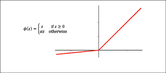
Here, ![]() determines the slope for the negative (preactivation) inputs.
determines the slope for the negative (preactivation) inputs.
We will define two helper functions for each of the two networks, instantiate a model from the Keras Sequential class, and add the layers as described. The code is as follows:
>>> import tensorflow as tf
>>> import tensorflow_datasets as tfds
>>> import numpy as np
>>> import matplotlib.pyplot as plt
>>> ## define a function for the generator:
>>> def make_generator_network(
...         num_hidden_layers=1,
...         num_hidden_units=100,
...         num_output_units=784):
...
...     model = tf.keras.Sequential()
...     for i in range(num_hidden_layers):
...         model.add(
...             tf.keras.layers.Dense(
...                 units=num_hidden_units, use_bias=False))
...         model.add(tf.keras.layers.LeakyReLU())
...
...     model.add(
...         tf.keras.layers.Dense(
...             units=num_output_units, activation='tanh'))
...     return model
>>> ## define a function for the discriminator:
>>> def make_discriminator_network(
...         num_hidden_layers=1,
...         num_hidden_units=100,
...         num_output_units=1):
...
...     model = tf.keras.Sequential()
...     for i in range(num_hidden_layers):
...         model.add(
...             tf.keras.layers.Dense(units=num_hidden_units))
...         model.add(tf.keras.layers.LeakyReLU())
...         model.add(tf.keras.layers.Dropout(rate=0.5))
...
...     model.add(
...         tf.keras.layers.Dense(
...             units=num_output_units, activation=None))
...     return model
Next, we will specify the training settings for the model. As you will remember from previous chapters, the image size in the MNIST dataset is ![]() pixels. (That is only one color channel because MNIST contains only grayscale images.) We will further specify the size of the input vector, z, to be 20, and we will use a random uniform distribution to initialize the model weights. Since we are implementing a very simple GAN model for illustration purposes only and using fully connected layers, we will only use a single hidden layer with 100 units in each network. In the following code, we will specify and initialize the two networks, and print their summary information:
pixels. (That is only one color channel because MNIST contains only grayscale images.) We will further specify the size of the input vector, z, to be 20, and we will use a random uniform distribution to initialize the model weights. Since we are implementing a very simple GAN model for illustration purposes only and using fully connected layers, we will only use a single hidden layer with 100 units in each network. In the following code, we will specify and initialize the two networks, and print their summary information:
>>> image_size = (28, 28)
>>> z_size = 20
>>> mode_z = 'uniform' # 'uniform' vs. 'normal'
>>> gen_hidden_layers = 1
>>> gen_hidden_size = 100
>>> disc_hidden_layers = 1
>>> disc_hidden_size = 100
>>> tf.random.set_seed(1)
>>> gen_model = make_generator_network(
...     num_hidden_layers=gen_hidden_layers,
...     num_hidden_units=gen_hidden_size,
...     num_output_units=np.prod(image_size))
>>> gen_model.build(input_shape=(None, z_size))
>>> gen_model.summary()
Model: "sequential"
_________________________________________________________________
Layer (type)                 Output Shape              Param #
=================================================================
dense (Dense)                multiple                  2000
_________________________________________________________________
leaky_re_lu (LeakyReLU)      multiple                  0
_________________________________________________________________
dense_1 (Dense)              multiple                  79184
=================================================================
Total params: 81,184
Trainable params: 81,184
Non-trainable params: 0
_________________________________________________________________
>>> disc_model = make_discriminator_network(
...     num_hidden_layers=disc_hidden_layers,
...     num_hidden_units=disc_hidden_size)
>>> disc_model.build(input_shape=(None, np.prod(image_size)))
>>> disc_model.summary()
Model: "sequential_1"
_________________________________________________________________
Layer (type)                 Output Shape              Param #
=================================================================
dense_2 (Dense)              multiple                  78500
_________________________________________________________________
leaky_re_lu_1 (LeakyReLU)    multiple                  0
_________________________________________________________________
dropout (Dropout)            multiple                  0
_________________________________________________________________
dense_3 (Dense)              multiple                  101
=================================================================
Total params: 78,601
Trainable params: 78,601
Non-trainable params: 0
_________________________________________________________________
Defining the training dataset
In the next step, we will load the MNIST dataset and apply the necessary preprocessing steps. Since the output layer of the generator is using the tanh activation function, the pixel values of the synthesized images will be in the range (–1, 1). However, the input pixels of the MNIST images are within the range [0, 255] (with a TensorFlow data type tf.uint8). Thus, in the preprocessing steps, we will use the tf.image.convert_image_dtype function to convert the dtype of the input image tensors from tf.uint8 to tf.float32. As a result, besides changing the dtype, calling this function will also change the range of input pixel intensities to [0, 1]. Then, we can scale them by a factor of 2 and shift them by –1 such that the pixel intensities will be rescaled to be in the range [–1, 1]. Furthermore, we will also create a random vector, z, based on the desired random distribution (in this code example, uniform or normal, which are the most common choices), and return both the preprocessed image and the random vector in a tuple:
>>> mnist_bldr = tfds.builder('mnist')
>>> mnist_bldr.download_and_prepare()
>>> mnist = mnist_bldr.as_dataset(shuffle_files=False)
>>> def preprocess(ex, mode='uniform'):
...     image = ex['image']
...     image = tf.image.convert_image_dtype(image, tf.float32)
...     image = tf.reshape(image, [-1])
...     image = image*2 - 1.0
...     if mode == 'uniform':
...         input_z = tf.random.uniform(
...             shape=(z_size,), minval=-1.0, maxval=1.0)
...     elif mode == 'normal':
...         input_z = tf.random.normal(shape=(z_size,))
...     return input_z, image
>>> mnist_trainset = mnist['train']
>>> mnist_trainset = mnist_trainset.map(preprocess)
Note that, here, we returned both the input vector, z, and the image to fetch the training data conveniently during model fitting. However, this does not imply that the vector, z, is by any means related to the image—the input image comes from the dataset, while vector z is generated randomly. In each training iteration, the randomly generated vector, z, represents the input that the generator receives for synthesizing a new image, and the images (the real ones as well as the synthesized ones) are the inputs to the discriminator.
Let's inspect the dataset object that we created. In the following code, we will take one batch of examples and print the array shapes of this sample of input vectors and images. Furthermore, in order to understand the overall data flow of our GAN model, in the following code, we will process a forward pass for our generator and discriminator.
First, we will feed the batch of input, z, vectors to the generator and get its output, g_output. This will be a batch of fake examples, which will be fed to the discriminator model to get the logits for the batch of fake examples, d_logits_fake. Furthermore, the processed images that we get from the dataset object will be fed to the discriminator model, which will result in the logits for the real examples, d_logits_real. The code is as follows:
>>> mnist_trainset = mnist_trainset.batch(32, drop_remainder=True)
>>> input_z, input_real = next(iter(mnist_trainset))
>>> print('input-z -- shape:   ', input_z.shape)
>>> print('input-real -- shape:', input_real.shape)
input-z -- shape:    (32, 20)
input-real -- shape: (32, 784)
>>> g_output = gen_model(input_z)
>>> print('Output of G -- shape:', g_output.shape)
Output of G -- shape: (32, 784)
>>> d_logits_real = disc_model(input_real)
>>> d_logits_fake = disc_model(g_output)
>>> print('Disc. (real) -- shape:', d_logits_real.shape)
>>> print('Disc. (fake) -- shape:', d_logits_fake.shape)
Disc. (real) -- shape: (32, 1)
Disc. (fake) -- shape: (32, 1)
The two logits, d_logits_fake and d_logits_real, will be used to compute the loss functions for training the model.
Training the GAN model
As the next step, we will create an instance of BinaryCrossentropy as our loss function and use that to calculate the loss for the generator and discriminator associated with the batches that we just processed. To do this, we also need the ground truth labels for each output. For the generator, we will create a vector of 1s with the same shape as the vector containing the predicted logits for the generated images, d_logits_fake. For the discriminator loss, we have two terms: the loss for detecting the fake examples involving d_logits_fake and the loss for detecting the real examples based on d_logits_real.
The ground truth labels for the fake term will be a vector of 0s that we can generate via the tf.zeros()(or tf.zeros_like()) function. Similarly, we can generate the ground truth values for the real images via the tf.ones()(or tf.ones_like()) function, which creates a vector of 1s:
>>> loss_fn = tf.keras.losses.BinaryCrossentropy(from_logits=True)
>>> ## Loss for the Generator
>>> g_labels_real = tf.ones_like(d_logits_fake)
>>> g_loss = loss_fn(y_true=g_labels_real, y_pred=d_logits_fake)
>>> print('Generator Loss: {:.4f}'.format(g_loss))
Generator Loss: 0.7505
>>> ## Loss for the Discriminator
>>> d_labels_real = tf.ones_like(d_logits_real)
>>> d_labels_fake = tf.zeros_like(d_logits_fake)
>>> d_loss_real = loss_fn(y_true=d_labels_real,
...                       y_pred=d_logits_real)
>>> d_loss_fake = loss_fn(y_true=d_labels_fake,
...                       y_pred=d_logits_fake)
>>> print('Discriminator Losses: Real {:.4f} Fake {:.4f}'
...       .format(d_loss_real.numpy(), d_loss_fake.numpy()))
Discriminator Losses: Real 1.3683 Fake 0.6434
The previous code example shows the step-by-step calculation of the different loss terms for the purpose of understanding the overall concept behind training a GAN model. The following code will set up the GAN model and implement the training loop, where we will include these calculations in a for loop.
In addition, we will use tf.GradientTape() to compute the loss gradients with respect to the model weights and optimize the parameters of the generator and discriminator using two separate Adam optimizers. As you will see in the following code, for alternating between the training of the generator and the discriminator in TensorFlow, we explicitly provide the parameters of each network and apply the gradients of each network separately to the respective designated optimizer:
>>> import time
>>> num_epochs = 100
>>> batch_size = 64
>>> image_size = (28, 28)
>>> z_size = 20
>>> mode_z = 'uniform'
>>> gen_hidden_layers = 1
>>> gen_hidden_size = 100
>>> disc_hidden_layers = 1
>>> disc_hidden_size = 100
>>> tf.random.set_seed(1)
>>> np.random.seed(1)
>>> if mode_z == 'uniform':
...     fixed_z = tf.random.uniform(
...         shape=(batch_size, z_size),
...         minval=-1, maxval=1)
>>> elif mode_z == 'normal':
...     fixed_z = tf.random.normal(
...         shape=(batch_size, z_size))
>>> def create_samples(g_model, input_z):
...     g_output = g_model(input_z, training=False)
...     images = tf.reshape(g_output, (batch_size, *image_size))
...     return (images+1)/2.0
>>> ## Set-up the dataset
>>> mnist_trainset = mnist['train']
>>> mnist_trainset = mnist_trainset.map(
...     lambda ex: preprocess(ex, mode=mode_z))
>>> mnist_trainset = mnist_trainset.shuffle(10000)
>>> mnist_trainset = mnist_trainset.batch(
...     batch_size, drop_remainder=True)
>>> ## Set-up the model
>>> with tf.device(device_name):
...     gen_model = make_generator_network(
...         num_hidden_layers=gen_hidden_layers,
...         num_hidden_units=gen_hidden_size,
...         num_output_units=np.prod(image_size))
...     gen_model.build(input_shape=(None, z_size))
...
...     disc_model = make_discriminator_network(
...         num_hidden_layers=disc_hidden_layers,
...         num_hidden_units=disc_hidden_size)
...     disc_model.build(input_shape=(None, np.prod(image_size)))
>>> ## Loss function and optimizers:
>>> loss_fn = tf.keras.losses.BinaryCrossentropy(from_logits=True)
>>> g_optimizer = tf.keras.optimizers.Adam()
>>> d_optimizer = tf.keras.optimizers.Adam()
>>> all_losses = []
>>> all_d_vals = []
>>> epoch_samples = []
>>> start_time = time.time()
>>> for epoch in range(1, num_epochs+1):
...
...     epoch_losses, epoch_d_vals = [], []
...
...     for i,(input_z,input_real) in enumerate(mnist_trainset):
...
...         ## Compute generator's loss
...         with tf.GradientTape() as g_tape:
...             g_output = gen_model(input_z)
...             d_logits_fake = disc_model(g_output,
...                                        training=True)
...             labels_real = tf.ones_like(d_logits_fake)
...             g_loss = loss_fn(y_true=labels_real,
...                              y_pred=d_logits_fake)
...
...         ## Compute the gradients of g_loss
...         g_grads = g_tape.gradient(g_loss,
...                       gen_model.trainable_variables)
...
...         ## Optimization: Apply the gradients
...         g_optimizer.apply_gradients(
...             grads_and_vars=zip(g_grads,
...             gen_model.trainable_variables))
...
...         ## Compute discriminator's loss
...         with tf.GradientTape() as d_tape:
...             d_logits_real = disc_model(input_real,
...                                        training=True)
...
...             d_labels_real = tf.ones_like(d_logits_real)
...
...             d_loss_real = loss_fn(
...                 y_true=d_labels_real, y_pred=d_logits_real)
...
...             d_logits_fake = disc_model(g_output,
...                                        training=True)
...             d_labels_fake = tf.zeros_like(d_logits_fake)
...
...             d_loss_fake = loss_fn(
...                 y_true=d_labels_fake, y_pred=d_logits_fake)
...
...             d_loss = d_loss_real + d_loss_fake
...
...         ## Compute the gradients of d_loss
...         d_grads = d_tape.gradient(d_loss,
...                       disc_model.trainable_variables)
...
...         ## Optimization: Apply the gradients
...         d_optimizer.apply_gradients(
...             grads_and_vars=zip(d_grads,
...             disc_model.trainable_variables))
...
...         epoch_losses.append(
...             (g_loss.numpy(), d_loss.numpy(),
...              d_loss_real.numpy(), d_loss_fake.numpy()))
...
...         d_probs_real = tf.reduce_mean(
...                            tf.sigmoid(d_logits_real))
...         d_probs_fake = tf.reduce_mean(
...                            tf.sigmoid(d_logits_fake))
...         epoch_d_vals.append((d_probs_real.numpy(),
...                              d_probs_fake.numpy()))
...
...     all_losses.append(epoch_losses)
...     all_d_vals.append(epoch_d_vals)
...     print(
...         'Epoch {:03d} | ET {:.2f} min | Avg Losses >>'
...         ' G/D {:.4f}/{:.4f} [D-Real: {:.4f} D-Fake: {:.4f}]'
...         .format(
...             epoch, (time.time() - start_time)/60,
...             *list(np.mean(all_losses[-1], axis=0))))
...     epoch_samples.append(
...         create_samples(gen_model, fixed_z).numpy())
Epoch 001 | ET 0.88 min | Avg Losses >> G/D 2.9594/0.2843 [D-Real: 0.0306 D-Fake: 0.2537]
Epoch 002 | ET 1.77 min | Avg Losses >> G/D 5.2096/0.3193 [D-Real: 0.1002 D-Fake: 0.2191]
Epoch ...
Epoch 100 | ET 88.25 min | Avg Losses >> G/D 0.8909/1.3262 [D-Real: 0.6655 D-Fake: 0.6607]
Using a GPU, the training process that we implemented in the previous code block should be completed in less than an hour on Google Colab. (It may even be faster on your personal computer if you have a recent and capable CPU and a GPU.) After the model training has completed, it is often helpful to plot the discriminator and generator losses to analyze the behavior of both subnetworks and assess whether they converged.
It is also helpful to plot the average probabilities of the batches of real and fake examples as computed by the discriminator in each iteration. We expect these probabilities to be around 0.5, which means that the discriminator is not able to confidently distinguish between real and fake images:
>>> import itertools
>>> fig = plt.figure(figsize=(16, 6))
>>> ## Plotting the losses
>>> ax = fig.add_subplot(1, 2, 1)
>>> g_losses = [item[0] for item in itertools.chain(*all_losses)]
>>> d_losses = [item[1]/2.0 for item in itertools.chain(
...             *all_losses)]
>>> plt.plot(g_losses, label='Generator loss', alpha=0.95)
>>> plt.plot(d_losses, label='Discriminator loss', alpha=0.95)
>>> plt.legend(fontsize=20)
>>> ax.set_xlabel('Iteration', size=15)
>>> ax.set_ylabel('Loss', size=15)
>>> epochs = np.arange(1, 101)
>>> epoch2iter = lambda e: e*len(all_losses[-1])
>>> epoch_ticks = [1, 20, 40, 60, 80, 100]
>>> newpos = [epoch2iter(e) for e in epoch_ticks]
>>> ax2 = ax.twiny()
>>> ax2.set_xticks(newpos)
>>> ax2.set_xticklabels(epoch_ticks)
>>> ax2.xaxis.set_ticks_position('bottom')
>>> ax2.xaxis.set_label_position('bottom')
>>> ax2.spines['bottom'].set_position(('outward', 60))
>>> ax2.set_xlabel('Epoch', size=15)
>>> ax2.set_xlim(ax.get_xlim())
>>> ax.tick_params(axis='both', which='major', labelsize=15)
>>> ax2.tick_params(axis='both', which='major', labelsize=15)
>>> ## Plotting the outputs of the discriminator
>>> ax = fig.add_subplot(1, 2, 2)
>>> d_vals_real = [item[0] for item in itertools.chain(
...                *all_d_vals)]
>>> d_vals_fake = [item[1] for item in itertools.chain(
...                *all_d_vals)]
>>> plt.plot(d_vals_real, alpha=0.75,
...          label=r'Real: $D(mathbf{x})$')
>>> plt.plot(d_vals_fake, alpha=0.75,
...          label=r'Fake: $D(G(mathbf{z}))$')
>>> plt.legend(fontsize=20)
>>> ax.set_xlabel('Iteration', size=15)
>>> ax.set_ylabel('Discriminator output', size=15)
>>> ax2 = ax.twiny()
>>> ax2.set_xticks(newpos)
>>> ax2.set_xticklabels(epoch_ticks)
>>> ax2.xaxis.set_ticks_position('bottom')
>>> ax2.xaxis.set_label_position('bottom')
>>> ax2.spines['bottom'].set_position(('outward', 60))
>>> ax2.set_xlabel('Epoch', size=15)
>>> ax2.set_xlim(ax.get_xlim())
>>> ax.tick_params(axis='both', which='major', labelsize=15)
>>> ax2.tick_params(axis='both', which='major', labelsize=15)
>>> plt.show()
The following figure shows the results:
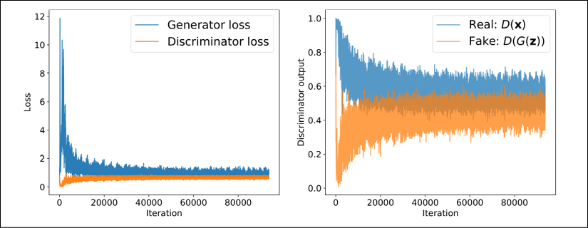
Note that the discriminator model outputs logits, but for this visualization, we already stored the probabilities computed via the sigmoid function before calculating the averages for each batch.
As you can see from the discriminator outputs in the previous figure, during the early stages of the training, the discriminator was able to quickly learn to distinguish quite accurately between the real and fake examples, that is, the fake examples had probabilities close to 0, and the real examples had probabilities close to 1. The reason for that was that the fake examples were nothing like the real ones; therefore, distinguishing between real and fake was rather easy. As the training proceeds further, the generator will become better at synthesizing realistic images, which will result in probabilities of both real and fake examples that are close to 0.5.
Furthermore, we can also see how the outputs of the generator, that is, the synthesized images, change during training. After each epoch, we generated some examples by calling the create_samples() function and stored them in a Python list. In the following code, we will visualize some of the images produced by the generator for a selection of epochs:
>>> selected_epochs = [1, 2, 4, 10, 50, 100]
>>> fig = plt.figure(figsize=(10, 14))
>>> for i,e in enumerate(selected_epochs):
...     for j in range(5):
...         ax = fig.add_subplot(6, 5, i*5+j+1)
...         ax.set_xticks([])
...         ax.set_yticks([])
...         if j == 0:
...             ax.text(
...                 -0.06, 0.5, 'Epoch {}'.format(e),
...                 rotation=90, size=18, color='red',
...                 horizontalalignment='right',
...                 verticalalignment='center',
...                 transform=ax.transAxes)
...
...         image = epoch_samples[e-1][j]
...         ax.imshow(image, cmap='gray_r')
...
>>> plt.show()
The following figure shows the produced images:

As you can see from the previous figure, the generator network produced more and more realistic images as the training progressed. However, even after 100 epochs, the produced images still look very different to the handwritten digits contained in the MNIST dataset.
In this section, we designed a very simple GAN model with only a single fully connected hidden layer for both the generator and discriminator. After training the GAN model on the MNIST dataset, we were able to achieve promising, although not yet satisfactory, results with the new handwritten digits. As we learned in Chapter 15, Classifying Images with Deep Convolutional Neural Networks, NN architectures with convolutional layers have several advantages over fully connected layers when it comes to image classification. In a similar sense, adding convolutional layers to our GAN model to work with image data might improve the outcome. In the next section, we will implement a deep convolutional GAN (DCGAN), which uses convolutional layers for both the generator and the discriminator networks.
Improving the quality of synthesized images using a convolutional and Wasserstein GAN
In this section, we will implement a DCGAN, which will enable us to improve the performance we saw in the previous GAN example. Additionally, we will employ several extra key techniques and implement a Wasserstein GAN (WGAN).
The techniques that we will cover in this section will include the following:
- Transposed convolution
- BatchNorm
- WGAN
- Gradient penalty
The DCGAN was proposed in 2016 by A. Radford, L. Metz, and S. Chintala in their article Unsupervised representation learning with deep convolutional generative adversarial networks, which is freely available at https://arxiv.org/pdf/1511.06434.pdf. In this article, the researchers proposed using convolutional layers for both the generator and discriminator networks. Starting from a random vector, z, the DCGAN first uses a fully connected layer to project z into a new vector with a proper size so that it can be reshaped into a spatial convolution representation (![]() ), which is smaller than the output image size. Then, a series of convolutional layers, known as transposed convolution, are used to upsample the feature maps to the desired output image size.
), which is smaller than the output image size. Then, a series of convolutional layers, known as transposed convolution, are used to upsample the feature maps to the desired output image size.
Transposed convolution
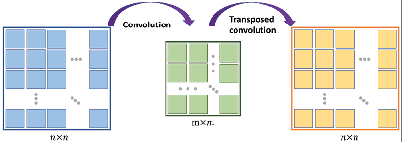
In Chapter 15, Classifying Images with Deep Convolutional Neural Networks, you learned about the convolution operation in one- and two-dimensional spaces. In particular, we looked at how the choices for the padding and strides change the output feature maps. While a convolution operation is usually used to downsample the feature space (for example, by setting the stride to 2, or by adding a pooling layer after a convolutional layer), a transposed convolution operation is usually used for upsampling the feature space.
To understand the transposed convolution operation, let's go through a simple thought experiment. Assume that we have an input feature map of size ![]() . Then, we apply a 2D convolution operation with certain padding and stride parameters to this
. Then, we apply a 2D convolution operation with certain padding and stride parameters to this ![]() input, resulting in an output feature map of size
input, resulting in an output feature map of size ![]() . Now, the question is, how we can apply another convolution operation to obtain a feature map with the initial dimension
. Now, the question is, how we can apply another convolution operation to obtain a feature map with the initial dimension ![]() from this
from this ![]() output feature map while maintaining the connectivity patterns between the input and output? Note that only the shape of the
output feature map while maintaining the connectivity patterns between the input and output? Note that only the shape of the ![]() input matrix is recovered and not the actual matrix values. This is what transposed convolution does, as shown in the following figure:
input matrix is recovered and not the actual matrix values. This is what transposed convolution does, as shown in the following figure:
Transposed convolution versus deconvolution
Transposed convolution is also called fractionally strided convolution. In deep learning literature, another common term that is used to refer to transposed convolution is deconvolution. However, note that deconvolution was originally defined as the inverse of a convolution operation, f, on a feature map, x, with weight parameters, w, producing feature map ![]() ,
, ![]() . A deconvolution function,
. A deconvolution function, ![]() , can then be defined as
, can then be defined as ![]() . However, note that the transposed convolution is merely focused on recovering the dimensionality of the feature space and not the actual values.
. However, note that the transposed convolution is merely focused on recovering the dimensionality of the feature space and not the actual values.
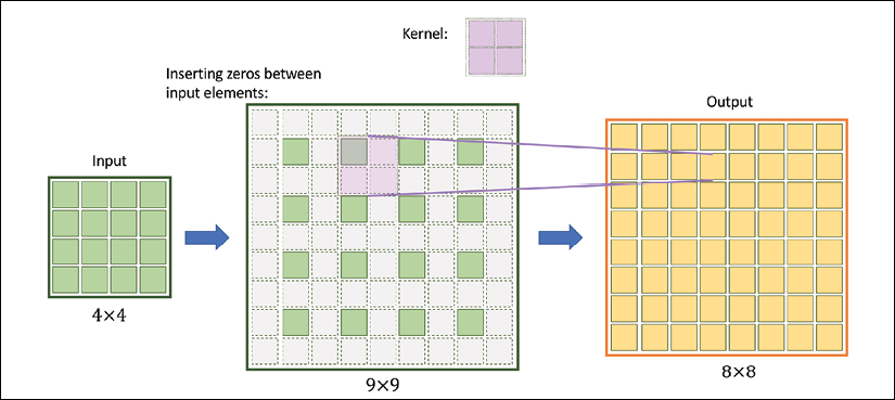
Upsampling feature maps using transposed convolution works by inserting 0s between the elements of the input feature maps. The following illustration shows an example of applying transposed convolution to an input of size ![]() , with a stride of
, with a stride of ![]() and kernel size of
and kernel size of ![]() . The matrix of size
. The matrix of size ![]() in the center shows the results after inserting such 0s into the input feature map. Then, performing a normal convolution using the
in the center shows the results after inserting such 0s into the input feature map. Then, performing a normal convolution using the ![]() kernel with a stride of 1 results in an output of size
kernel with a stride of 1 results in an output of size ![]() . We can verify the backward direction by performing a regular convolution on the output with a stride of 2, which results in an output feature map of size
. We can verify the backward direction by performing a regular convolution on the output with a stride of 2, which results in an output feature map of size ![]() , which is the same as the original input size:
, which is the same as the original input size:
The preceding illustration shows how transposed convolution works in general. There are various cases in which input size, kernel size, strides, and padding variations can change the output. If you want to learn more about all these different cases, refer to the tutorial A Guide to Convolution Arithmetic for Deep Learning by Vincent Dumoulin and Francesco Visin, which is freely available at https://arxiv.org/pdf/1603.07285.pdf.
Batch normalization
BatchNorm was introduced in 2015 by Sergey Ioffe and Christian Szegedy in the article Batch Normalization: Accelerating Deep Network Training by Reducing Internal Covariate Shift, which you can access via arXiv at https://arxiv.org/pdf/1502.03167.pdf. One of the main ideas behind BatchNorm is normalizing the layer inputs and preventing changes in their distribution during training, which enables faster and better convergence.
BatchNorm transforms a mini-batch of features based on its computed statistics. Assume that we have the net preactivation feature maps obtained after a convolutional layer in a four-dimensional tensor, Z, with the shape ![]() , where m is the number of examples in the batch (i.e., batch size),
, where m is the number of examples in the batch (i.e., batch size), ![]() is the spatial dimension of the feature maps, and c is the number of channels. BatchNorm can be summarized in three steps, as follows:
is the spatial dimension of the feature maps, and c is the number of channels. BatchNorm can be summarized in three steps, as follows:
- Compute the mean and standard deviation of the net inputs for each mini-batch:
 ,
,  , where
  and
and  both have size c.
 - Standardize the net inputs for all examples in the batch:
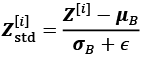 , where
  is a small number for numerical stability (that is, to avoid division by zero).
 - Scale and shift the normalized net inputs using two learnable parameter vectors,
 and
and  , of size c (number of channels):
  .
.
The following figure illustrates the process:

In the first step of BatchNorm, the mean, ![]() , and standard deviation,
, and standard deviation, ![]() , of the mini-batch are computed. Both
, of the mini-batch are computed. Both ![]() and
and ![]() are vectors of size c (where c is the number of channels). Then, these statistics are used in step 2 to scale the examples in each mini-batch via z-score normalization (standardization), resulting in standardized net inputs,
are vectors of size c (where c is the number of channels). Then, these statistics are used in step 2 to scale the examples in each mini-batch via z-score normalization (standardization), resulting in standardized net inputs, ![]() . As a consequence, these net inputs are mean-centered and have unit variance, which is generally a useful property for gradient descent-based optimization. On the other hand, always normalizing the net inputs such that they have the same properties across the different mini-batches, which can be diverse, can severely impact the representational capacity of NNs. This can be understood by considering a feature,
. As a consequence, these net inputs are mean-centered and have unit variance, which is generally a useful property for gradient descent-based optimization. On the other hand, always normalizing the net inputs such that they have the same properties across the different mini-batches, which can be diverse, can severely impact the representational capacity of NNs. This can be understood by considering a feature, ![]() , which, after sigmoid activation to
, which, after sigmoid activation to ![]() , results in a linear region for values close to 0. Therefore, in step 3, the learnable parameters,
, results in a linear region for values close to 0. Therefore, in step 3, the learnable parameters, ![]() and
and ![]() , which are vectors of size c (number of channels), allow BatchNorm to control the shift and spread of the normalized features.
, which are vectors of size c (number of channels), allow BatchNorm to control the shift and spread of the normalized features.
During training, the running averages, ![]() , and running variance,
, and running variance, ![]() , are computed, which are used along with the tuned parameters,
, are computed, which are used along with the tuned parameters, ![]() and
and ![]() , to normalize the test example(s) at evaluation.
, to normalize the test example(s) at evaluation.
Why does BatchNorm help optimization?
Initially, BatchNorm was developed to reduce the so-called internal covariance shift, which is defined as the changes that occur in the distribution of a layer's activations due to the updated network parameters during training.
To explain this with a simple example, consider a fixed batch that passes through the network at epoch 1. We record the activations of each layer for this batch. After iterating through the whole training dataset and updating the model parameters, we start the second epoch, where the previously fixed batch passes through the network. Then, we compare the layer activations from the first and second epochs. Since the network parameters have changed, we observe that the activations have also changed. This phenomenon is called the internal covariance shift, which was believed to decelerate NN training.
However, in 2018, S. Santurkar, D. Tsipras, A. Ilyas, and A. Madry further investigated what makes BatchNorm so effective. In their study, the researchers observed that the effect of BatchNorm on the internal covariance shift is marginal. Based on the outcome of their experiments, they hypothesized that the effectiveness of BatchNorm is, instead, based on a smoother surface of the loss function, which makes the non-convex optimization more robust.
If you are interested in learning more about these results, read through the original paper, How Does Batch Normalization Help Optimization?, which is freely available at http://papers.nips.cc/paper/7515-how-does-batch-normalization-help-optimization.pdf.
The TensorFlow Keras API provides a class, tf.keras.layers.BatchNormalization(), that we can use as a layer when defining our models; it will perform all of the steps that we described for BatchNorm. Note that the behavior for updating the learnable parameters, ![]() and
and ![]() , depends on whether
, depends on whether training=False or training=True, which can be used to ensure that these parameters are learned only during training.
Implementing the generator and discriminator
At this point, we have covered the main components of a DCGAN model, which we will now implement. The architectures of the generator and discriminator networks are summarized in the following two figures.
The generator takes a vector, z, of size 20 as input, applies a fully connected (dense) layer to increase its size to 6,272 and then reshapes it into a rank-3 tensor of shape ![]() (spatial dimension
(spatial dimension ![]() and 128 channels). Then, a series of transposed convolutions using
and 128 channels). Then, a series of transposed convolutions using tf.keras.layers.Conv2DTransposed() upsamples the feature maps until the spatial dimension of the resulting feature maps reaches ![]() . The number of channels is reduced by half after each transposed convolutional layer, except the last one, which uses only one output filter to generate a grayscale image. Each transposed convolutional layer is followed by BatchNorm and leaky ReLU activation functions, except the last one, which uses tanh activation (without BatchNorm). The architecture for the generator (the feature maps after each layer) is shown in the following figure:
. The number of channels is reduced by half after each transposed convolutional layer, except the last one, which uses only one output filter to generate a grayscale image. Each transposed convolutional layer is followed by BatchNorm and leaky ReLU activation functions, except the last one, which uses tanh activation (without BatchNorm). The architecture for the generator (the feature maps after each layer) is shown in the following figure:

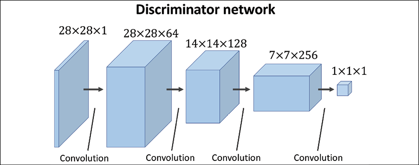
The discriminator receives images of size ![]() , which are passed through four convolutional layers. The first three convolutional layers reduce the spatial dimensionality by 4 while increasing the number of channels of the feature maps. Each convolutional layer is also followed by BatchNorm, leaky ReLU activation, and a dropout layer with
, which are passed through four convolutional layers. The first three convolutional layers reduce the spatial dimensionality by 4 while increasing the number of channels of the feature maps. Each convolutional layer is also followed by BatchNorm, leaky ReLU activation, and a dropout layer with rate=0.3 (drop probability). The last convolutional layer uses kernels of size ![]() and a single filter to reduce the spatial dimensionality of the output to
and a single filter to reduce the spatial dimensionality of the output to ![]() :
:
Architecture design considerations for convolutional GANs
Notice that the number of feature maps follows different trends between the generator and the discriminator. In the generator, we start with a large number of feature maps and decrease them as we progress toward the last layer. On the other hand, in the discriminator, we start with a small number of channels and increase it toward the last layer. This is an important point for designing CNNs with the number of feature maps and the spatial size of the feature maps in reverse order. When the spatial size of the feature maps increases, the number of feature maps decreases and vice versa.
In addition, note that it's usually not recommended to use bias units in the layer that follows a BatchNorm layer. Using bias units would be redundant in this case, since BatchNorm already has a shift parameter, ![]() . You can omit the bias units for a given layer by setting
. You can omit the bias units for a given layer by setting use_bias=False in tf.keras.layers.Dense or tf.keras.layers.Conv2D.
The code for two helper functions to make the generator and discriminator networks is as follows:
>>> def make_dcgan_generator(
...         z_size=20,
...         output_size=(28, 28, 1),
...         n_filters=128,
...         n_blocks=2):
...     size_factor = 2**n_blocks
...     hidden_size = (
...         output_size[0]//size_factor,
...         output_size[1]//size_factor)
...
...     model = tf.keras.Sequential([
...         tf.keras.layers.Input(shape=(z_size,)),
...
...         tf.keras.layers.Dense(
...             units=n_filters*np.prod(hidden_size),
...             use_bias=False),
...         tf.keras.layers.BatchNormalization(),
...         tf.keras.layers.LeakyReLU(),
...         tf.keras.layers.Reshape(
...             (hidden_size[0], hidden_size[1], n_filters)),
...
...         tf.keras.layers.Conv2DTranspose(
...             filters=n_filters, kernel_size=(5, 5),
...             strides=(1, 1), padding='same', use_bias=False),
...         tf.keras.layers.BatchNormalization(),
...         tf.keras.layers.LeakyReLU()
...     ])
...
...     nf = n_filters
...     for i in range(n_blocks):
...         nf = nf // 2
...         model.add(
...             tf.keras.layers.Conv2DTranspose(
...                 filters=nf, kernel_size=(5, 5),
...                 strides=(2, 2), padding='same',
...                 use_bias=False))
...         model.add(tf.keras.layers.BatchNormalization())
...         model.add(tf.keras.layers.LeakyReLU())
...
...     model.add(
...         tf.keras.layers.Conv2DTranspose(
...             filters=output_size[2], kernel_size=(5, 5),
...             strides=(1, 1), padding='same', use_bias=False,
...             activation='tanh'))
...
...     return model
>>> def make_dcgan_discriminator(
...         input_size=(28, 28, 1),
...         n_filters=64,
...         n_blocks=2):
...     model = tf.keras.Sequential([
...         tf.keras.layers.Input(shape=input_size),
...         tf.keras.layers.Conv2D(
...             filters=n_filters, kernel_size=5,
...             strides=(1, 1), padding='same'),
...         tf.keras.layers.BatchNormalization(),
...         tf.keras.layers.LeakyReLU()
...     ])
...
...     nf = n_filters
...     for i in range(n_blocks):
...         nf = nf*2
...         model.add(
...             tf.keras.layers.Conv2D(
...                 filters=nf, kernel_size=(5, 5),
...                 strides=(2, 2),padding='same'))
...         model.add(tf.keras.layers.BatchNormalization())
...         model.add(tf.keras.layers.LeakyReLU())
...         model.add(tf.keras.layers.Dropout(0.3))
...
...     model.add(
...         tf.keras.layers.Conv2D(
...                 filters=1, kernel_size=(7, 7),
...                 padding='valid'))
...
...     model.add(tf.keras.layers.Reshape((1,)))
...
...     return model
With these two helper functions, you can build a DCGAN model and train it by using the same MNIST dataset object we initialized in the previous section when we implemented the simple, fully connected GAN. Also, we can use the same loss functions and training procedure as before.
We will be making a few additional modifications to the DCGAN model in the remaining sections of this chapter. Note that the preprocess() function for transforming the dataset must change to output an image tensor instead of flattening the image to a vector. The following code shows the necessary modifications to build the dataset, as well as creating the new generator and discriminator networks:
>>> mnist_bldr = tfds.builder('mnist')
>>> mnist_bldr.download_and_prepare()
>>> mnist = mnist_bldr.as_dataset(shuffle_files=False)
>>> def preprocess(ex, mode='uniform'):
...     image = ex['image']
...     image = tf.image.convert_image_dtype(image, tf.float32)
...
...     image = image*2 - 1.0
...     if mode == 'uniform':
...         input_z = tf.random.uniform(
...             shape=(z_size,), minval=-1.0, maxval=1.0)
...     elif mode == 'normal':
...         input_z = tf.random.normal(shape=(z_size,))
...     return input_z, image
We can create the generator networks using the helper function, make_dcgan_generator(), and print its architecture as follows:
>>> gen_model = make_dcgan_generator()
>>> gen_model.summary()
Model: "sequential_2"
_________________________________________________________________
Layer (type)                 Output Shape              Param #
=================================================================
dense_1 (Dense)              (None, 6272)              125440
_________________________________________________________________
batch_normalization_7 (Batch (None, 6272)              25088
_________________________________________________________________
leaky_re_lu_7 (LeakyReLU)    (None, 6272)              0
_________________________________________________________________
reshape_2 (Reshape)          (None, 7, 7, 128)         0
_________________________________________________________________
conv2d_transpose_4 (Conv2DTr (None, 7, 7, 128)         409600
_________________________________________________________________
batch_normalization_8 (Batch (None, 7, 7, 128)         512
_________________________________________________________________
leaky_re_lu_8 (LeakyReLU)    (None, 7, 7, 128)         0
_________________________________________________________________
conv2d_transpose_5 (Conv2DTr (None, 14, 14, 64)        204800
_________________________________________________________________
batch_normalization_9 (Batch (None, 14, 14, 64)        256
_________________________________________________________________
leaky_re_lu_9 (LeakyReLU)    (None, 14, 14, 64)        0
_________________________________________________________________
conv2d_transpose_6 (Conv2DTr (None, 28, 28, 32)        51200
_________________________________________________________________
batch_normalization_10 (Batc (None, 28, 28, 32)        128
_________________________________________________________________
leaky_re_lu_10 (LeakyReLU)   (None, 28, 28, 32)        0
_________________________________________________________________
conv2d_transpose_7 (Conv2DTr (None, 28, 28, 1)         800
=================================================================
Total params: 817,824
Trainable params: 804,832
Non-trainable params: 12,992
_________________________________________________________________
Similarly, we can generate the discriminator network and see its architecture:
>>> disc_model = make_dcgan_discriminator()
>>> disc_model.summary()
Model: "sequential_3"
_________________________________________________________________
Layer (type)                 Output Shape              Param #
=================================================================
conv2d_4 (Conv2D)            (None, 28, 28, 64)        1664
_________________________________________________________________
batch_normalization_11 (Batc (None, 28, 28, 64)        256
_________________________________________________________________
leaky_re_lu_11 (LeakyReLU)   (None, 28, 28, 64)        0
_________________________________________________________________
conv2d_5 (Conv2D)            (None, 14, 14, 128)       204928
_________________________________________________________________
batch_normalization_12 (Batc (None, 14, 14, 128)       512
_________________________________________________________________
leaky_re_lu_12 (LeakyReLU)   (None, 14, 14, 128)       0
_________________________________________________________________
dropout_2 (Dropout)          (None, 14, 14, 128)       0
_________________________________________________________________
conv2d_6 (Conv2D)            (None, 7, 7, 256)         819456
_________________________________________________________________
batch_normalization_13 (Batc (None, 7, 7, 256)         1024
_________________________________________________________________
leaky_re_lu_13 (LeakyReLU)   (None, 7, 7, 256)         0
_________________________________________________________________
dropout_3 (Dropout)          (None, 7, 7, 256)         0
_________________________________________________________________
conv2d_7 (Conv2D)            (None, 1, 1, 1)           12545
_________________________________________________________________
reshape_3 (Reshape)          (None, 1)                 0
=================================================================
Total params: 1,040,385
Trainable params: 1,039,489
Non-trainable params: 896
_________________________________________________________________
Notice that the number of parameters for the BatchNorm layers is indeed four times the number of channels (![]() ). Remember that the BatchNorm parameters,
). Remember that the BatchNorm parameters, ![]() and
and ![]() , represent the (non-trainable parameters) mean and standard deviation for each feature value inferred from a given batch;
, represent the (non-trainable parameters) mean and standard deviation for each feature value inferred from a given batch; ![]() and
and ![]() are the trainable BN parameters.
are the trainable BN parameters.
Note that this particular architecture would not perform very well when using cross-entropy as a loss function.
In the next subsection, we will cover WGAN, which uses a modified loss function based on the so-called Wasserstein-1 (or earth mover's) distance between the distributions of real and fake images for improving the training performance.
Dissimilarity measures between two distributions
We will first see different measures for computing the divergence between two distributions. Then, we will see which one of these measures is already embedded in the original GAN model. Finally, switching this measure in GANs will lead us to the implementation of a WGAN.
As mentioned at the beginning of this chapter, the goal of a generative model is to learn how to synthesize new samples that have the same distribution as the distribution of the training dataset. Let P(x) and Q(x) represent the distribution of a random variable, x, as shown in the following figure.
First, let's look at some ways, shown in the following figure, that we can use to measure the dissimilarity between two distributions, P and Q:
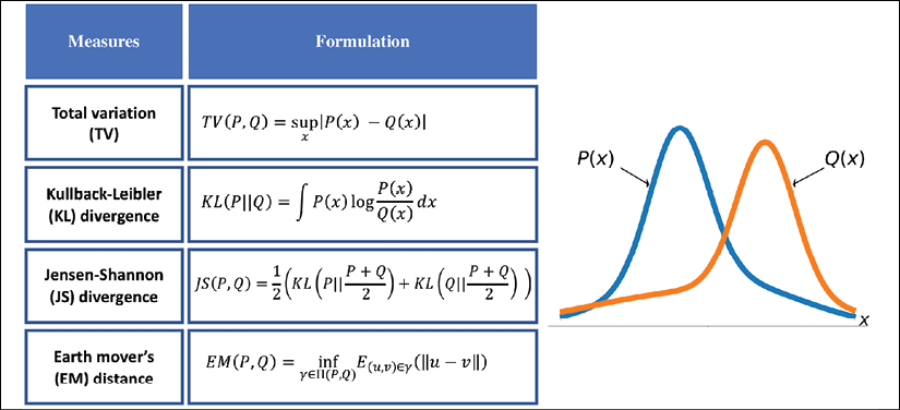
The function supremum, sup(S), used in the total variation (TV) measure, refers to the smallest value that is greater than all elements of S. In other words, sup(S) is the least upper bound for S. Vice versa, the infimum function, inf(S), which is used in EM distance, refers to the largest value that is smaller than all elements of S (the greatest lower bound). Let's gain an understanding of these measures by briefly stating what they are trying to accomplish in simple words:
- The first one, TV distance, measures the largest difference between the two distributions at each point.
- The EM distance can be interpreted as the minimal amount of work needed to transform one distribution into the other. The infimum function in the EM distance is taken over
 , which is the collection of all joint distributions whose marginals are P or Q. Then,
  is a transfer plan, which indicates how we redistribute the earth from location u to v, subject to some constraints for maintaining valid distributions after such transfers. Computing EM distance is an optimization problem by itself, which is to find the optimal transfer plan,
  .
. - The Kullback-Leibler (KL) and Jensen-Shannon (JS) divergence measures come from the field of information theory. Note that KL divergence is not symmetric, that is,
 in contrast to JS divergence.
The dissimilarity equations provided in the previous figure correspond to continuous distributions but can be extended for discrete cases. An example of calculating these different dissimilarity measures with two simple discrete distributions is illustrated in the following figure:
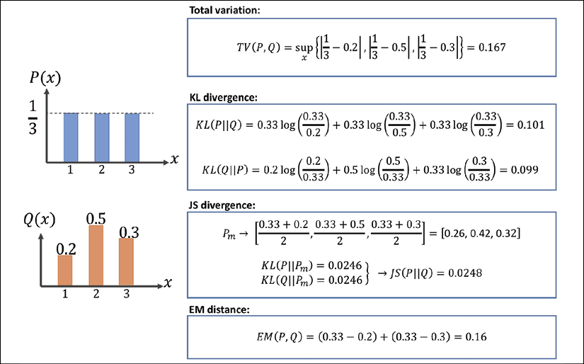
Note that, in the case of the EM distance, for this simple example, we can see that Q(x) at x = 2 has the excess value of  , while the value of Q at the other two x's is below 1/3. Therefore, the minimal amount of work is when we transfer the extra value at x = 2 to x = 1 and x = 3, as shown in the previous figure. For this simple example, it's easy to see that these transfers will result in the minimal amount of work out of all possible transfers. However, this may be infeasible to do for more complex cases.
The relationship between KL divergence and cross-entropy
KL divergence, ![]() , measures the relative entropy of the distribution, P, with respect to a reference distribution, Q. The formulation for KL divergence can be extended as
, measures the relative entropy of the distribution, P, with respect to a reference distribution, Q. The formulation for KL divergence can be extended as

Moreover, for discrete distributions, KL divergence can be written as

which can be similarly extended as
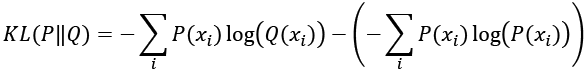
Based on the extended formulation (either discrete or continuous), KL divergence is viewed as the cross-entropy between P and Q (the first term in the preceding equation) subtracted by the (self-) entropy of P (second term), that is, ![]() .
.
Now, going back to our discussion of GANs, let's see how these different distance measures are related to the loss function for GANs. It can be mathematically shown that the loss function in the original GAN indeed minimizes the JS divergence between the distribution of real and fake examples. But, as discussed in an article by Martin Arjovsky et al. (Wasserstein Generative Adversarial Networks, http://proceedings.mlr.press/v70/arjovsky17a/arjovsky17a.pdf), JS divergence has problems training a GAN model, and therefore, in order to improve the training, the researchers proposed using the EM distance as a measure of dissimilarity between the distribution of real and fake examples.
What is the advantage of using EM distance?
To answer this question, we can consider an example that was given in the article by Martin Arjovsky et al, titled Wasserstein GAN. To put it in simple words, assume we have two distributions, P and Q, which are two parallel lines. One line is fixed at x = 0 and the other line can move across the x-axis but is initially located at ![]() , where
, where ![]() .
.
It can be shown that the KL, TV, and JS dissimilarity measures are ![]() ,
, ![]() , and
, and ![]() . None of these dissimilarity measures are a function of the parameter
. None of these dissimilarity measures are a function of the parameter ![]() , and therefore, they cannot be differentiated with respect to
, and therefore, they cannot be differentiated with respect to ![]() toward making the distributions, P and Q, become similar to each other. On the other hand, the EM distance is
toward making the distributions, P and Q, become similar to each other. On the other hand, the EM distance is ![]() , whose gradient with respect to
, whose gradient with respect to ![]() exists and can push Q toward P.
exists and can push Q toward P.
Now, let's focus our attention on how EM distance can be used to train a GAN model. Let's assume ![]() is the distribution of the real examples and
is the distribution of the real examples and ![]() denotes the distributions of fake (generated) examples.
denotes the distributions of fake (generated) examples. ![]() and
and ![]() replace P and Q in the EM distance equation. As was mentioned earlier, computing the EM distance is an optimization problem by itself; therefore, this becomes computationally intractable, especially if we want to repeat this computation in each iteration of the GAN training loop. Fortunately, though, the computation of the EM distance can be simplified using a theorem called Kantorovich-Rubinstein duality, as follows:
replace P and Q in the EM distance equation. As was mentioned earlier, computing the EM distance is an optimization problem by itself; therefore, this becomes computationally intractable, especially if we want to repeat this computation in each iteration of the GAN training loop. Fortunately, though, the computation of the EM distance can be simplified using a theorem called Kantorovich-Rubinstein duality, as follows:

Here, the supremum is taken over all the 1-Lipschitz continuous functions denoted by ![]() .
.
Lipschitz continuity
Based on 1-Lipschitz continuity, the function, f, must satisfy the following property:

Furthermore, a real function, ![]() , that satisfies the property
, that satisfies the property
is called K-Lipschitz continuous.
Using EM distance in practice for GANs
Now, the question is, how do we find such a 1-Lipschitz continuous function to compute the Wasserstein distance between the distribution of real (![]() ) and fake (
) and fake (![]() ) outputs for a GAN? While the theoretical concepts behind the WGAN approach may seem complicated at first, the answer to this question is simpler than it may appear. Recall that we consider deep NNs to be universal function approximators. This means that we can simply train an NN model to approximate the Wasserstein distance function. As you saw in the previous section, the simple GAN uses a discriminator in the form of a classifier. For WGAN, the discriminator can be changed to behave as a critic, which returns a scalar score instead of a probability value. We can interpret this score as how realistic the input images are (like an art critic giving scores to artworks in a gallery).
) outputs for a GAN? While the theoretical concepts behind the WGAN approach may seem complicated at first, the answer to this question is simpler than it may appear. Recall that we consider deep NNs to be universal function approximators. This means that we can simply train an NN model to approximate the Wasserstein distance function. As you saw in the previous section, the simple GAN uses a discriminator in the form of a classifier. For WGAN, the discriminator can be changed to behave as a critic, which returns a scalar score instead of a probability value. We can interpret this score as how realistic the input images are (like an art critic giving scores to artworks in a gallery).
To train a GAN using the Wasserstein distance, the losses for the discriminator, D, and generator, G, are defined as follows. The critic (that is, the discriminator network) returns its outputs for the batch of real image examples and the batch of synthesized examples. We use the notations D(x) and D(G(z)), respectively. Then, the following loss terms can be defined:
- The real component of the discriminator's loss:
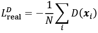
- The fake component of the discriminator's loss:
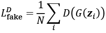
- The loss for the generator:

That will be all for the WGAN, except that we need to ensure that the 1-Lipschitz property of the critic function is preserved during training. For this purpose, the WGAN paper proposes clamping the weights to a small region, for example, [–0.01, 0.01].
Gradient penalty
In the paper by Arjovsky et al., weight clipping is suggested for the 1-Lipschitz property of the discriminator (or critic). However, in another paper titled Improved Training of Wasserstein GANs, which is freely available at https://arxiv.org/pdf/1704.00028.pdf, Ishaan Gulrajani et al. showed that clipping the weights can lead to exploding and vanishing gradients. Furthermore, weight clipping can also lead to capacity underuse, which means that the critic network is limited to learning only some simple functions, as opposed to more complex functions. Therefore, rather than clipping the weights, Ishaan Guljarani et al. proposed gradient penalty (GP) as an alternative solution. The result is the WGAN with gradient penalty (WGAN-GP).
The procedure for the GP that is added in each iteration can be summarized by the following sequence of steps:
- For each pair of real and fake examples
 in a given batch, choose a random number,
  , sampled from a uniform distribution, that is,
 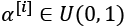 .
. - Calculate an interpolation between the real and fake examples:
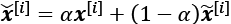 , resulting in a batch of interpolated examples.
 - Compute the discriminator (critic) output for all the interpolated examples,
 .
. - Calculate the gradients of the critic's output with respect to each interpolated example, that is,
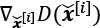 .
. - Compute the GP as
 .
.
The total loss for the discriminator is then as follows:
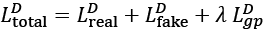 ,
,Here, ![]() is a tunable hyperparameter.
is a tunable hyperparameter.
Implementing WGAN-GP to train the DCGAN model
We have already defined the helper functions that create the generator and discriminator networks for DCGAN (make_dcgan_generator() and make_dcgan_discriminator()). The code to build the DCGAN model is as follows:
>>> num_epochs = 100
>>> batch_size = 128
>>> image_size = (28, 28)
>>> z_size = 20
>>> mode_x = 'uniform'
>>> lambda_gp = 10.0
>>> tf.random.set_seed(1)
>>> np.random.seed(1)
>>> ## Set-up the dataset
>>> mnist_trainset = mnist['train']
>>> mnist_trainset = mnist_trainset.map(preprocess)
>>> mnist_trainset = mnist_trainset.shuffle(10000)
>>> mnist_trainset = mnist_trainset.batch(
...     batch_size, drop_remainder=True)
>>> ## Set-up the model
>>> with tf.device(device_name):
...     gen_model = make_dcgan_generator()
...     gen_model.build(input_shape=(None, z_size))
...
...     disc_model = make_dcgan_discriminator()
...     disc_model.build(input_shape=(None, np.prod(image_size)))
Now we can train the model. Note that, typically, the RMSprop optimizer is recommended for WGAN (without the GP), whereas the Adam optimizer is used for WGAN-GP. The code is as follows:
>>> import time
>>> ## Optimizers:
>>> g_optimizer = tf.keras.optimizers.Adam(0.0002)
>>> d_optimizer = tf.keras.optimizers.Adam(0.0002)
>>> if mode_z == 'uniform':
...     fixed_z = tf.random.uniform(
...         shape=(batch_size, z_size), minval=-1, maxval=1)
... elif mode_z == 'normal':
...     fixed_z = tf.random.normal(shape=(batch_size, z_size))
...
>>> def create_samples(g_model, input_z):
...     g_output = g_model(input_z, training=False)
...     images = tf.reshape(g_output, (batch_size, *image_size))
...     return (images+1)/2.0
>>> all_losses = []
>>> epoch_samples = []
>>> start_time = time.time()
>>> for epoch in range(1, num_epochs+1):
...
...     epoch_losses = []
...
...     for i,(input_z,input_real) in enumerate(mnist_trainset):
...
...         with tf.GradientTape() as d_tape, tf.GradientTape()
...                 as g_tape:
...
...             g_output = gen_model(input_z, training=True)
...
...             d_critics_real = disc_model(input_real,
...                 training=True)
...             d_critics_fake = disc_model(g_output,
...                 training=True)
...
...             ## Compute generator's loss:
...             g_loss = -tf.math.reduce_mean(d_critics_fake)
...
...             ## compute discriminator's losses:
...             d_loss_real = -tf.math.reduce_mean(d_critics_real)
...             d_loss_fake =  tf.math.reduce_mean(d_critics_fake)
...             d_loss = d_loss_real + d_loss_fake
...
...             ## Gradient-penalty:
...             with tf.GradientTape() as gp_tape:
...                 alpha = tf.random.uniform(
...                     shape=[d_critics_real.shape[0], 1, 1, 1],
...                     minval=0.0, maxval=1.0)
...                 interpolated = (alpha*input_real +
...                                  (1-alpha)*g_output)
...                 gp_tape.watch(interpolated)
...                 d_critics_intp = disc_model(interpolated)
...
...             grads_intp = gp_tape.gradient(
...                 d_critics_intp, [interpolated,])[0]
...             grads_intp_l2 = tf.sqrt(
...                 tf.reduce_sum(tf.square(grads_intp),
...                               axis=[1, 2, 3]))
...             grad_penalty = tf.reduce_mean(tf.square(
...                                grads_intp_l2 - 1.0))
...
...             d_loss = d_loss + lambda_gp*grad_penalty
...
...         ## Optimization: Compute the gradients apply them
...         d_grads = d_tape.gradient(d_loss,
...                       disc_model.trainable_variables)
...         d_optimizer.apply_gradients(
...             grads_and_vars=zip(d_grads,
...             disc_model.trainable_variables))
...
...         g_grads = g_tape.gradient(g_loss,
...                       gen_model.trainable_variables)
...         g_optimizer.apply_gradients(
...             grads_and_vars=zip(g_grads,
...             gen_model.trainable_variables))
...
...         epoch_losses.append(
...             (g_loss.numpy(), d_loss.numpy(),
...              d_loss_real.numpy(), d_loss_fake.numpy()))
...
...     all_losses.append(epoch_losses)
...     print(
...         'Epoch {:03d} | ET {:.2f} min | Avg Losses >>'
...         ' G/D {:6.2f}/{:6.2f} [D-Real: {:6.2f}'
...         ' D-Fake: {:6.2f}]'
...         .format(
...             epoch, (time.time() - start_time)/60,
...             *list(np.mean(all_losses[-1], axis=0))))
...     epoch_samples.append(
...         create_samples(gen_model, fixed_z).numpy())
Finally, let's visualize the saved examples at some epochs to see how the model is learning and how the quality of synthesized examples changes over the course of learning:
>>> selected_epochs = [1, 2, 4, 10, 50, 100]
>>> fig = plt.figure(figsize=(10, 14))
>>> for i,e in enumerate(selected_epochs):
...     for j in range(5):
...         ax = fig.add_subplot(6, 5, i*5+j+1)
...         ax.set_xticks([])
...         ax.set_yticks([])
...         if j == 0:
...             ax.text(-0.06, 0.5, 'Epoch {}'.format(e),
...                     rotation=90, size=18, color='red',
...                     horizontalalignment='right',
...                     verticalalignment='center',
...                     transform=ax.transAxes)
...
...         image = epoch_samples[e-1][j]
...         ax.imshow(image, cmap='gray_r')
>>> plt.show()
The following figure shows the results:
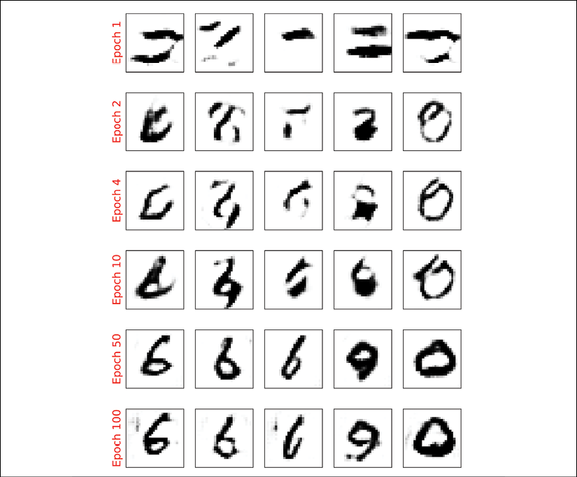
We used the same code to visualize the results as in the section on vanilla GAN. Comparing the new examples shows that DCGAN (with Wasserstein and GP) can generate images of a much higher quality.
Mode collapse
Due to the adversarial nature of GAN models, it is notoriously hard to train them. One common cause of failure in training GANs is when the generator gets stuck in a small subspace and learns to generate similar samples. This is called mode collapse, and an example is shown in the following figure.
The synthesized examples in this figure are not cherry-picked. This shows that the generator has failed to learn the entire data distribution, and instead, has taken a lazy approach focusing on a subspace:

Besides the vanishing and exploding gradient problems that we saw previously, there are some further aspects that can also make training GAN models difficult (indeed, it is an art). Here are a few suggested tricks from GAN artists.
One approach is called mini-batch discrimination, which is based on the fact that batches consisting of only real or fake examples are fed separately to the discriminator. In mini-batch discrimination, we let the discriminator compare examples across these batches to see whether a batch is real or fake. The diversity of a batch consisting of only real examples is most likely higher than the diversity of a fake batch if a model suffers from mode collapse.
Another technique that is commonly used for stabilizing GAN training is feature matching. In feature matching, we make a slight modification to the objective function of the generator by adding an extra term that minimizes the difference between the original and synthesized images based on intermediate representations (feature maps) of the discriminator. We encourage you to read more about this technique in the original article by Ting-Chun Wang et al., titled High Resolution Image Synthesis and Semantic Manipulation with Conditional GANs, which is freely available at https://arxiv.org/pdf/1711.11585.pdf.
During the training, a GAN model can also get stuck in several modes and just hop between them. To avoid this behavior, you can store some old examples and feed them to the discriminator to prevent the generator from revisiting previous modes. This technique is referred to as experience replay. Furthermore, you can train multiple GANs with different random seeds so that the combination of all of them covers a larger part of the data distribution than any single one of them.
Other GAN applications
In this chapter, we mainly focused on generating examples using GANs and looked at a few tricks and techniques to improve the quality of synthesized outputs. The applications of GANs are expanding rapidly, including in computer vision, machine learning, and even other domains of science and engineering. A nice list of different GAN models and application areas can be found at https://github.com/hindupuravinash/the-gan-zoo.
It is worth mentioning that we covered GANs in an unsupervised fashion, that is, no class label information was used in the models that were covered in this chapter. However, the GAN approach can be generalized to semi-supervised and supervised tasks, as well. For example, the conditional GAN (cGAN) proposed by Mehdi Mirza and Simon Osindero in the paper Conditional Generative Adversarial Nets (https://arxiv.org/pdf/1411.1784.pdf) uses the class label information and learns to synthesize new images conditioned on the provided label, that is, ![]() —applied to MNIST. This allows us to generate different digits in the range 0-9 selectively. Furthermore, conditional GANs allows us to do image-to-image translation, which is to learn how to convert a given image from a specific domain to another. In this context, one interesting work is the Pix2Pix algorithm, published in the paper Image-to-Image Translation with Conditional Adversarial Networks by Philip Isola et al. (https://arxiv.org/pdf/1611.07004.pdf). It is worth mentioning that in the Pix2Pix algorithm, the discriminator provides the real/fake predictions for multiple patches across the image as opposed to a single prediction for an entire image.
—applied to MNIST. This allows us to generate different digits in the range 0-9 selectively. Furthermore, conditional GANs allows us to do image-to-image translation, which is to learn how to convert a given image from a specific domain to another. In this context, one interesting work is the Pix2Pix algorithm, published in the paper Image-to-Image Translation with Conditional Adversarial Networks by Philip Isola et al. (https://arxiv.org/pdf/1611.07004.pdf). It is worth mentioning that in the Pix2Pix algorithm, the discriminator provides the real/fake predictions for multiple patches across the image as opposed to a single prediction for an entire image.
CycleGAN is another interesting GAN model built on top of the cGAN, also for image-to-image translation. However, note that in CycleGAN, the training examples from the two domains are unpaired, meaning that there is no one-to-one correspondence between inputs and outputs. For example, using a CycleGAN, we could change the season of a picture taken in summer to winter. In the paper Unpaired Image-to-Image Translation Using Cycle-Consistent Adversarial Networks by Jun-Yan Zhu et al. (https://arxiv.org/pdf/1703.10593.pdf), an impressive example shows horses converted into zebras.
Summary
In this chapter, you first learned about generative models in deep learning and their overall objective: synthesizing new data. We then covered how GAN models use a generator network and a discriminator network, which compete with each other in an adversarial training setting to improve each other. Next, we implemented a simple GAN model using only fully connected layers for both the generator and the discriminator.
We also covered how GAN models can be improved. First, you saw a DCGAN, which uses deep convolutional networks for both the generator and the discriminator. Along the way, you also learned about two new concepts: transposed convolution (for upsampling the spatial dimensionality of feature maps) and BatchNorm (for improving convergence during training).
We then looked at a WGAN, which uses the EM distance to measure the distance between the distributions of real and fake samples. Finally, we talked about the WGAN with GP to maintain the 1-Lipschitz property instead of clipping the weights.
In the next chapter, we will look at reinforcement learning, which is a completely different category of machine learning compared to what we have covered so far in this book.