In the modern internet and social media age, people's opinions, reviews, and recommendations have become a valuable resource for political science and businesses. Thanks to modern technologies, we are now able to collect and analyze such data most efficiently. In this chapter, we will delve into a subfield of natural language processing (NLP) called sentiment analysis and learn how to use machine learning algorithms to classify documents based on their polarity: the attitude of the writer. In particular, we are going to work with a dataset of 50,000 movie reviews from the Internet Movie Database (IMDb) and build a predictor that can distinguish between positive and negative reviews.

The topics that we will cover in the following sections include the following:

• Cleaning and preparing text data
• Building feature vectors from text documents
• Training a machine learning model to classify positive and negative movie reviews
• Working with large text datasets using out-of-core learning
• Inferring topics from document collections for categorization

Preparing the IMDb movie review data for text processing

As mentioned, sentiment analysis, sometimes also called opinion mining, is a popular subdiscipline of the broader field of NLP; it is concerned with analyzing the polarity of documents. A popular task in sentiment analysis is the classification of documents based on the expressed opinions or emotions of the authors with regard to a particular topic.

In this chapter, we will be working with a large dataset of movie reviews from the Internet Movie Database (IMDb) that has been collected by Andrew Maas and others (Learning Word Vectors for Sentiment Analysis, A. L. Maas, R. E. Daly, P. T. Pham, D. Huang, A. Y. Ng, and C. Potts, Proceedings of the 49th Annual Meeting of the Association for Computational Linguistics: Human Language Technologies, pages 142–150, Portland, Oregon, USA, Association for Computational Linguistics, June 2011). The movie review dataset consists of 50,000 polar movie reviews that are labeled as either positive or negative; here, positive means that a movie was rated with more than six stars on IMDb, and negative means that a movie was rated with fewer than five stars on IMDb. In the following sections, we will download the dataset, preprocess it into a useable format for machine learning tools, and extract meaningful information from a subset of these movie reviews to build a machine learning model that can predict whether a certain reviewer liked or disliked a movie.

Obtaining the movie review dataset

A compressed archive of the movie review dataset (84.1 MB) can be downloaded from http://ai.stanford.edu/~amaas/data/sentiment/ as a gzip-compressed tarball archive:

• If you are working with Linux or macOS, you can open a new terminal window, cd into the download directory and execute tar -zxf aclImdb_v1.tar.gz to decompress the dataset.
• If you are working with Windows, you can download a free archiver, such as 7-Zip (http://www.7-zip.org), to extract the files from the download archive.
• Alternatively, you can directly unpack the gzip-compressed tarball archive directly in Python as follows:

  >>> import tarfile
  >>> with tarfile.open('aclImdb_v1.tar.gz', 'r:gz') as tar:
  ...     tar.extractall()
  

Preprocessing the movie dataset into a more convenient format

Having successfully extracted the dataset, we will now assemble the individual text documents from the decompressed download archive into a single CSV file. In the following code section, we will be reading the movie reviews into a pandas DataFrame object, which can take up to 10 minutes on a standard desktop computer.

To visualize the progress and estimated time until completion, we will use the Python Progress Indicator (PyPrind, https://pypi.python.org/pypi/PyPrind/) package, which was developed several years ago for such purposes. PyPrind can be installed by executing the pip install pyprind command:

>>> import pyprind
>>> import pandas as pd
>>> import os
>>> # change the 'basepath' to the directory of the
>>> # unzipped movie dataset
>>> basepath = 'aclImdb'
>>>
>>> labels = {'pos': 1, 'neg': 0}
>>> pbar = pyprind.ProgBar(50000)
>>> df = pd.DataFrame()
>>> for s in ('test', 'train'):
...     for l in ('pos', 'neg'):
...         path = os.path.join(basepath, s, l)
...         for file in sorted(os.listdir(path)):
...             with open(os.path.join(path, file),
...                       'r', encoding='utf-8') as infile:
...                 txt = infile.read()
...             df = df.append([[txt, labels[l]]],
...                            ignore_index=True)
...             pbar.update()
>>> df.columns = ['review', 'sentiment']
0%                          100%
[##############################] | ETA: 00:00:00
Total time elapsed: 00:02:05

In the preceding code, we first initialized a new progress bar object, pbar, with 50,000 iterations, which was the number of documents we were going to read in. Using the nested for loops, we iterated over the train and test subdirectories in the main aclImdb directory and read the individual text files from the pos and neg subdirectories that we eventually appended to the df pandas DataFrame, together with an integer class label (1 = positive and 0 = negative).

Since the class labels in the assembled dataset are sorted, we will now shuffle DataFrame using the permutation function from the np.random submodule—this will be useful to split the dataset into training and test datasets in later sections, when we will stream the data from our local drive directly.

For our own convenience, we will also store the assembled and shuffled movie review dataset as a CSV file:

>>> import numpy as np
>>> np.random.seed(0)
>>> df = df.reindex(np.random.permutation(df.index))
>>> df.to_csv('movie_data.csv', index=False, encoding='utf-8')

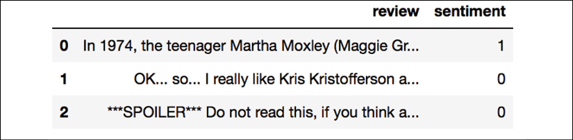
Since we are going to use this dataset later in this chapter, let's quickly confirm that we have successfully saved the data in the right format by reading in the CSV and printing an excerpt of the first three examples:

>>> df = pd.read_csv('movie_data.csv', encoding='utf-8')
>>> df.head(3)

If you are running the code examples in a Jupyter Notebook, you should now see the first three examples of the dataset, as shown in the following table:

As a sanity check, before we proceed to the next section, let's make sure that the DataFrame contains all 50,000 rows:

>>> df.shape
(50000, 2)

Introducing the bag-of-words model

You may remember from Chapter 4, Building Good Training Datasets – Data Preprocessing, that we have to convert categorical data, such as text or words, into a numerical form before we can pass it on to a machine learning algorithm. In this section, we will introduce the bag-of-words model, which allows us to represent text as numerical feature vectors. The idea behind bag-of-words is quite simple and can be summarized as follows:

1. We create a vocabulary of unique tokens—for example, words—from the entire set of documents.
2. We construct a feature vector from each document that contains the counts of how often each word occurs in the particular document.

Since the unique words in each document represent only a small subset of all the words in the bag-of-words vocabulary, the feature vectors will mostly consist of zeros, which is why we call them sparse. Do not worry if this sounds too abstract; in the following subsections, we will walk through the process of creating a simple bag-of-words model step by step.

Transforming words into feature vectors

To construct a bag-of-words model based on the word counts in the respective documents, we can use the CountVectorizer class implemented in scikit-learn. As you will see in the following code section, CountVectorizer takes an array of text data, which can be documents or sentences, and constructs the bag-of-words model for us:

>>> import numpy as np
>>> from sklearn.feature_extraction.text import CountVectorizer
>>> count = CountVectorizer()
>>> docs = np.array(['The sun is shining',
...                  'The weather is sweet',
...                  'The sun is shining, the weather is sweet,'
...                  'and one and one is two'])
>>> bag = count.fit_transform(docs)

By calling the fit_transform method on CountVectorizer, we constructed the vocabulary of the bag-of-words model and transformed the following three sentences into sparse feature vectors:

• 'The sun is shining'
• 'The weather is sweet'
• 'The sun is shining, the weather is sweet, and one and one is two'

Now, let's print the contents of the vocabulary to get a better understanding of the underlying concepts:

>>> print(count.vocabulary_)
{'and': 0,
'two': 7,
'shining': 3,
'one': 2,
'sun': 4,
'weather': 8,
'the': 6,
'sweet': 5,
'is': 1}

As you can see from executing the preceding command, the vocabulary is stored in a Python dictionary that maps the unique words to integer indices. Next, let's print the feature vectors that we just created:

>>> print(bag.toarray())
[[0 1 0 1 1 0 1 0 0]
 [0 1 0 0 0 1 1 0 1]
 [2 3 2 1 1 1 2 1 1]]

Each index position in the feature vectors shown here corresponds to the integer values that are stored as dictionary items in the CountVectorizer vocabulary. For example, the first feature at index position 0 resembles the count of the word 'and', which only occurs in the last document, and the word 'is', at index position 1 (the second feature in the document vectors), occurs in all three sentences. These values in the feature vectors are also called the raw term frequencies: tf(t, d)—the number of times a term, t, occurs in a document, d. It should be noted that, in the bag-of-words model, the word or term order in a sentence or document does not matter. The order in which the term frequencies appear in the feature vector is derived from the vocabulary indices, which are usually assigned alphabetically.

Assessing word relevancy via term frequency-inverse document frequency

When we are analyzing text data, we often encounter words that occur across multiple documents from both classes. These frequently occurring words typically don't contain useful or discriminatory information. In this subsection, you will learn about a useful technique called the term frequency-inverse document frequency (tf-idf), which can be used to downweight these frequently occurring words in the feature vectors. The tf-idf can be defined as the product of the term frequency and the inverse document frequency:

Here, tf(t, d) is the term frequency that we introduced in the previous section, and idf(t, d) is the inverse document frequency, which can be calculated as follows:

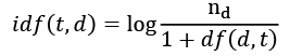
Here, is the total number of documents, and df(d, t) is the number of documents, d, that contain the term t. Note that adding the constant 1 to the denominator is optional and serves the purpose of assigning a non-zero value to terms that occur in none of the training examples; the log is used to ensure that low document frequencies are not given too much weight.

The scikit-learn library implements yet another transformer, the TfidfTransformer class, which takes the raw term frequencies from the CountVectorizer class as input and transforms them into tf-idfs:

>>> from sklearn.feature_extraction.text import TfidfTransformer
>>> tfidf = TfidfTransformer(use_idf=True,
...                          norm='l2',
...                          smooth_idf=True)
>>> np.set_printoptions(precision=2)
>>> print(tfidf.fit_transform(count.fit_transform(docs))
...       .toarray())
[[ 0.    0.43  0.    0.56  0.56  0.    0.43  0.    0.  ]
 [ 0.    0.43  0.    0.    0.    0.56  0.43  0.    0.56]
 [ 0.5   0.45  0.5   0.19  0.19  0.19  0.3   0.25  0.19]]

As you saw in the previous subsection, the word 'is' had the largest term frequency in the third document, being the most frequently occurring word. However, after transforming the same feature vector into tf-idfs, the word 'is' is now associated with a relatively small tf-idf (0.45) in the third document, since it is also present in the first and second document and thus is unlikely to contain any useful discriminatory information.

However, if we'd manually calculated the tf-idfs of the individual terms in our feature vectors, we would have noticed that TfidfTransformer calculates the tf-idfs slightly differently compared to the standard textbook equations that we defined previously. The equation for the inverse document frequency implemented in scikit-learn is computed as follows:

Similarly, the tf-idf computed in scikit-learn deviates slightly from the default equation we defined earlier:

Note that the "+1" in the previous equations is due to setting smooth_idf=True in the previous code example, which is helpful for assigning zero-weight (that is, idf(t, d) = log(1) = 0) to terms that occur in all documents.

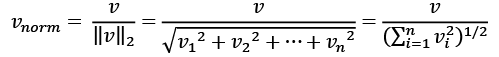
While it is also more typical to normalize the raw term frequencies before calculating the tf-idfs, the TfidfTransformer class normalizes the tf-idfs directly. By default (norm='l2'), scikit-learn's TfidfTransformer applies the L2-normalization, which returns a vector of length 1 by dividing an unnormalized feature vector, v, by its L2-norm:

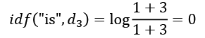
To make sure that we understand how TfidfTransformer works, let's walk through an example and calculate the tf-idf of the word 'is' in the third document. The word 'is' has a term frequency of 3 (tf = 3) in the third document, and the document frequency of this term is 3 since the term 'is' occurs in all three documents (df = 3). Thus, we can calculate the inverse document frequency as follows:

Now, in order to calculate the tf-idf, we simply need to add 1 to the inverse document frequency and multiply it by the term frequency:

If we repeated this calculation for all terms in the third document, we'd obtain the following tf-idf vectors: [3.39, 3.0, 3.39, 1.29, 1.29, 1.29, 2.0, 1.69, 1.29]. However, notice that the values in this feature vector are different from the values that we obtained from TfidfTransformer that we used previously. The final step that we are missing in this tf-idf calculation is the L2-normalization, which can be applied as follows:

As you can see, the results now match the results returned by scikit-learn's TfidfTransformer, and since you now understand how tf-idfs are calculated, let's proceed to the next section and apply those concepts to the movie review dataset.

Cleaning text data

In the previous subsections, we learned about the bag-of-words model, term frequencies, and tf-idfs. However, the first important step—before we build our bag-of-words model—is to clean the text data by stripping it of all unwanted characters.

To illustrate why this is important, let's display the last 50 characters from the first document in the reshuffled movie review dataset:

>>> df.loc[0, 'review'][-50:]
'is seven.<br /><br />Title (Brazil): Not Available'

As you can see here, the text contains HTML markup as well as punctuation and other non-letter characters. While HTML markup does not contain many useful semantics, punctuation marks can represent useful, additional information in certain NLP contexts. However, for simplicity, we will now remove all punctuation marks except for emoticon characters, such as :), since those are certainly useful for sentiment analysis. To accomplish this task, we will use Python's regular expression (regex) library, re, as shown here:

>>> import re
>>> def preprocessor(text):
...     text = re.sub('<[^>]*>', '', text)
...     emoticons = re.findall('(?::|;|=)(?:-)?(?:)|(|D|P)',
...                            text)
...     text = (re.sub('[W]+', ' ', text.lower()) +
...             ' '.join(emoticons).replace('-', ''))
...     return text

Via the first regex, <[^>]*>, in the preceding code section, we tried to remove all of the HTML markup from the movie reviews. Although many programmers generally advise against the use of regex to parse HTML, this regex should be sufficient to clean this particular dataset. Since we are only interested in removing HTML markup and do not plan to use the HTML markup further, using regex to do the job should be acceptable. However, if you prefer using sophisticated tools for removing HTML markup from text, you can take a look at Python's HTML parser module, which is described at https://docs.python.org/3/library/html.parser.html. After we removed the HTML markup, we used a slightly more complex regex to find emoticons, which we temporarily stored as emoticons. Next, we removed all non-word characters from the text via the regex [W]+ and converted the text into lowercase characters.

Eventually, we added the temporarily stored emoticons to the end of the processed document string. Additionally, we removed the nose character (- in :-)) from the emoticons for consistency.

Although the addition of the emoticon characters to the end of the cleaned document strings may not look like the most elegant approach, we must note that the order of the words doesn't matter in our bag-of-words model if our vocabulary consists of only one-word tokens. But before we talk more about the splitting of documents into individual terms, words, or tokens, let's confirm that our preprocessor function works correctly:

>>> preprocessor(df.loc[0, 'review'][-50:])
'is seven title brazil not available'
>>> preprocessor("</a>This :) is :( a test :-)!")
'this is a test :) :( :)'

Lastly, since we will make use of the cleaned text data over and over again during the next sections, let's now apply our preprocessor function to all the movie reviews in our DataFrame:

>>> df['review'] = df['review'].apply(preprocessor)

Processing documents into tokens

After successfully preparing the movie review dataset, we now need to think about how to split the text corpora into individual elements. One way to tokenize documents is to split them into individual words by splitting the cleaned documents at their whitespace characters:

>>> def tokenizer(text):
...     return text.split()
>>> tokenizer('runners like running and thus they run')
['runners', 'like', 'running', 'and', 'thus', 'they', 'run']

In the context of tokenization, another useful technique is word stemming, which is the process of transforming a word into its root form. It allows us to map related words to the same stem. The original stemming algorithm was developed by Martin F. Porter in 1979 and is hence known as the Porter stemmer algorithm (An algorithm for suffix stripping, Martin F. Porter, Program: Electronic Library and Information Systems, 14(3): 130–137, 1980). The Natural Language Toolkit (NLTK, http://www.nltk.org) for Python implements the Porter stemming algorithm, which we will use in the following code section. In order to install the NLTK, you can simply execute conda install nltk or pip install nltk.

The following code shows how to use the Porter stemming algorithm:

>>> from nltk.stem.porter import PorterStemmer
>>> porter = PorterStemmer()
>>> def tokenizer_porter(text):
...     return [porter.stem(word) for word in text.split()]
>>> tokenizer_porter('runners like running and thus they run')
['runner', 'like', 'run', 'and', 'thu', 'they', 'run']

Using the PorterStemmer from the nltk package, we modified our tokenizer function to reduce words to their root form, which was illustrated by the simple preceding example where the word 'running' was stemmed to its root form 'run'.

Before we jump into the next section, where we will train a machine learning model using the bag-of-words model, let's briefly talk about another useful topic called stop-word removal. Stop-words are simply those words that are extremely common in all sorts of texts and probably bear no (or only a little) useful information that can be used to distinguish between different classes of documents. Examples of stop-words are is, and, has, and like. Removing stop-words can be useful if we are working with raw or normalized term frequencies rather than tf-idfs, which are already downweighting frequently occurring words.

In order to remove stop-words from the movie reviews, we will use the set of 127 English stop-words that is available from the NLTK library, which can be obtained by calling the nltk.download function:

>>> import nltk
>>> nltk.download('stopwords')
After we download the stop-words set, we can load and apply the English stop-word set as follows:
>>> from nltk.corpus import stopwords
>>> stop = stopwords.words('english')
>>> [w for w in tokenizer_porter('a runner likes'
...  ' running and runs a lot')[-10:]
...  if w not in stop]
['runner', 'like', 'run', 'run', 'lot']

Training a logistic regression model for document classification

In this section, we will train a logistic regression model to classify the movie reviews into positive and negative reviews based on the bag-of-words model. First, we will divide the DataFrame of cleaned text documents into 25,000 documents for training and 25,000 documents for testing:

>>> X_train = df.loc[:25000, 'review'].values
>>> y_train = df.loc[:25000, 'sentiment'].values
>>> X_test = df.loc[25000:, 'review'].values
>>> y_test = df.loc[25000:, 'sentiment'].values

Next, we will use a GridSearchCV object to find the optimal set of parameters for our logistic regression model using 5-fold stratified cross-validation:

>>> from sklearn.model_selection import GridSearchCV
>>> from sklearn.pipeline import Pipeline
>>> from sklearn.linear_model import LogisticRegression
>>> from sklearn.feature_extraction.text import TfidfVectorizer
>>> tfidf = TfidfVectorizer(strip_accents=None,
...                         lowercase=False,
...                         preprocessor=None)
>>> param_grid = [{'vect__ngram_range': [(1,1)],
...                'vect__stop_words': [stop, None],
...                'vect__tokenizer': [tokenizer,
...                                    tokenizer_porter],
...                'clf__penalty': ['l1', 'l2'],
...                'clf__C': [1.0, 10.0, 100.0]},
...               {'vect__ngram_range': [(1,1)],
...                'vect__stop_words': [stop, None],
...                'vect__tokenizer': [tokenizer,
...                                    tokenizer_porter],
...                'vect__use_idf':[False],
...                'vect__norm':[None],
...                'clf__penalty': ['l1', 'l2'],
...                'clf__C': [1.0, 10.0, 100.0]}
...              ]
>>> lr_tfidf = Pipeline([('vect', tfidf),
...                      ('clf',
...                       LogisticRegression(random_state=0,
...                                          solver='liblinear'))])
>>> gs_lr_tfidf = GridSearchCV(lr_tfidf, param_grid,
...                            scoring='accuracy',
...                            cv=5, verbose=2,
...                            n_jobs=1)
>>> gs_lr_tfidf.fit(X_train, y_train)

When we initialized the GridSearchCV object and its parameter grid using the preceding code, we restricted ourselves to a limited number of parameter combinations, since the number of feature vectors, as well as the large vocabulary, can make the grid search computationally quite expensive. Using a standard desktop computer, our grid search may take up to 40 minutes to complete.

In the previous code example, we replaced CountVectorizer and TfidfTransformer from the previous subsection with TfidfVectorizer, which combines CountVectorizer with the TfidfTransformer. Our param_grid consisted of two parameter dictionaries. In the first dictionary, we used TfidfVectorizer with its default settings (use_idf=True, smooth_idf=True, and norm='l2') to calculate the tf-idfs; in the second dictionary, we set those parameters to use_idf=False, smooth_idf=False, and norm=None in order to train a model based on raw term frequencies. Furthermore, for the logistic regression classifier itself, we trained models using L2 and L1 regularization via the penalty parameter and compared different regularization strengths by defining a range of values for the inverse-regularization parameter C.

After the grid search has finished, we can print the best parameter set:

>>> print('Best parameter set: %s ' % gs_lr_tfidf.best_params_)
Best parameter set: {'clf__C': 10.0, 'vect__stop_words': None, 'clf__penalty': 'l2', 'vect__tokenizer': <function tokenizer at 0x7f6c704948c8>, 'vect__ngram_range': (1, 1)}

As you can see in the preceding output, we obtained the best grid search results using the regular tokenizer without Porter stemming, no stop-word library, and tf-idfs in combination with a logistic regression classifier that uses L2-regularization with the regularization strength C of 10.0.

Using the best model from this grid search, let's print the average 5-fold cross-validation accuracy scores on the training dataset and the classification accuracy on the test dataset:

>>> print('CV Accuracy: %.3f'
...       % gs_lr_tfidf.best_score_)
CV Accuracy: 0.897
>>> clf = gs_lr_tfidf.best_estimator_
>>> print('Test Accuracy: %.3f'
...       % clf.score(X_test, y_test))
Test Accuracy: 0.899

The results reveal that our machine learning model can predict whether a movie review is positive or negative with 90 percent accuracy.

Working with bigger data – online algorithms and out-of-core learning

If you executed the code examples in the previous section, you may have noticed that it could be computationally quite expensive to construct the feature vectors for the 50,000-movie review dataset during grid search. In many real-world applications, it is not uncommon to work with even larger datasets that can exceed our computer's memory. Since not everyone has access to supercomputer facilities, we will now apply a technique called out-of-core learning, which allows us to work with such large datasets by fitting the classifier incrementally on smaller batches of a dataset.

Back in Chapter 2, Training Simple Machine Learning Algorithms for Classification, the concept of stochastic gradient descent was introduced; it is an optimization algorithm that updates the model's weights using one example at a time. In this section, we will make use of the partial_fit function of SGDClassifier in scikit-learn to stream the documents directly from our local drive and train a logistic regression model using small mini-batches of documents.

First, we will define a tokenizer function that cleans the unprocessed text data from the movie_data.csv file that we constructed at the beginning of this chapter and separate it into word tokens while removing stop-words:

>>> import numpy as np
>>> import re
>>> from nltk.corpus import stopwords
>>> stop = stopwords.words('english')
>>> def tokenizer(text):
...     text = re.sub('<[^>]*>', '', text)
...     emoticons = re.findall('(?::|;|=)(?:-)?(?:)|(|D|P)',
...                            text.lower())
...     text = re.sub('[W]+', ' ', text.lower()) 
...                   + ' '.join(emoticons).replace('-', '')
...     tokenized = [w for w in text.split() if w not in stop]
...     return tokenized

Next, we will define a generator function, stream_docs, that reads in and returns one document at a time:

>>> def stream_docs(path):
...     with open(path, 'r', encoding='utf-8') as csv:
...         next(csv) # skip header
...         for line in csv:
...             text, label = line[:-3], int(line[-2])
...             yield text, label

To verify that our stream_docs function works correctly, let's read in the first document from the movie_data.csv file, which should return a tuple consisting of the review text as well as the corresponding class label:

>>> next(stream_docs(path='movie_data.csv'))
('"In 1974, the teenager Martha Moxley ... ',1)

We will now define a function, get_minibatch, that will take a document stream from the stream_docs function and return a particular number of documents specified by the size parameter:

>>> def get_minibatch(doc_stream, size):
...     docs, y = [], []
...     try:
...         for _ in range(size):
...             text, label = next(doc_stream)
...             docs.append(text)
...             y.append(label)
...     except StopIteration:
...         return None, None
...     return docs, y

Unfortunately, we can't use CountVectorizer for out-of-core learning since it requires holding the complete vocabulary in memory. Also, TfidfVectorizer needs to keep all the feature vectors of the training dataset in memory to calculate the inverse document frequencies. However, another useful vectorizer for text processing implemented in scikit-learn is HashingVectorizer. HashingVectorizer is data-independent and makes use of the hashing trick via the 32-bit MurmurHash3 function by Austin Appleby (https://sites.google.com/site/murmurhash/):

>>> from sklearn.feature_extraction.text import HashingVectorizer
>>> from sklearn.linear_model import SGDClassifier
>>> vect = HashingVectorizer(decode_error='ignore',
...                          n_features=2**21,
...                          preprocessor=None,
...                          tokenizer=tokenizer)
>>> clf = SGDClassifier(loss='log', random_state=1)
>>> doc_stream = stream_docs(path='movie_data.csv')

Using the preceding code, we initialized HashingVectorizer with our tokenizer function and set the number of features to 2**21. Furthermore, we reinitialized a logistic regression classifier by setting the loss parameter of SGDClassifier to 'log'. Note that by choosing a large number of features in HashingVectorizer, we reduce the chance of causing hash collisions, but we also increase the number of coefficients in our logistic regression model.

Now comes the really interesting part – having set up all the complementary functions, we can start the out-of-core learning using the following code:

>>> import pyprind
>>> pbar = pyprind.ProgBar(45)
>>> classes = np.array([0, 1])
>>> for _ in range(45):
...     X_train, y_train = get_minibatch(doc_stream, size=1000)
...     if not X_train:
...         break
...     X_train = vect.transform(X_train)
...     clf.partial_fit(X_train, y_train, classes=classes)
...     pbar.update()
0%                          100%
[##############################] | ETA: 00:00:00
Total time elapsed: 00:00:21

Again, we made use of the PyPrind package in order to estimate the progress of our learning algorithm. We initialized the progress bar object with 45 iterations and, in the following for loop, we iterated over 45 mini-batches of documents where each mini-batch consists of 1,000 documents. Having completed the incremental learning process, we will use the last 5,000 documents to evaluate the performance of our model:

>>> X_test, y_test = get_minibatch(doc_stream, size=5000)
>>> X_test = vect.transform(X_test)
>>> print('Accuracy: %.3f' % clf.score(X_test, y_test))
Accuracy: 0.868

As you can see, the accuracy of the model is approximately 87 percent, slightly below the accuracy that we achieved in the previous section using the grid search for hyperparameter tuning. However, out-of-core learning is very memory efficient and it took less than a minute to complete. Finally, we can use the last 5,000 documents to update our model:

>>> clf = clf.partial_fit(X_test, y_test)

Topic modeling with Latent Dirichlet Allocation

Topic modeling describes the broad task of assigning topics to unlabeled text documents. For example, a typical application would be the categorization of documents in a large text corpus of newspaper articles. In applications of topic modeling, we then aim to assign category labels to those articles, for example, sports, finance, world news, politics, local news, and so forth. Thus, in the context of the broad categories of machine learning that we discussed in Chapter 1, Giving Computers the Ability to Learn from Data, we can consider topic modeling as a clustering task, a subcategory of unsupervised learning.

In this section, we will discuss a popular technique for topic modeling called Latent Dirichlet Allocation (LDA). However, note that while Latent Dirichlet Allocation is often abbreviated as LDA, it is not to be confused with linear discriminant analysis, a supervised dimensionality reduction technique that was introduced in Chapter 5, Compressing Data via Dimensionality Reduction.

Decomposing text documents with LDA

Since the mathematics behind LDA is quite involved and requires knowledge about Bayesian inference, we will approach this topic from a practitioner's perspective and interpret LDA using layman's terms. However, the interested reader can read more about LDA in the following research paper: Latent Dirichlet Allocation, David M. Blei, Andrew Y. Ng, and Michael I. Jordan, Journal of Machine Learning Research 3, pages: 993-1022, Jan 2003.

LDA is a generative probabilistic model that tries to find groups of words that appear frequently together across different documents. These frequently appearing words represent our topics, assuming that each document is a mixture of different words. The input to an LDA is the bag-of-words model that we discussed earlier in this chapter. Given a bag-of-words matrix as input, LDA decomposes it into two new matrices:

• A document-to-topic matrix
• A word-to-topic matrix

LDA decomposes the bag-of-words matrix in such a way that if we multiply those two matrices together, we will be able to reproduce the input, the bag-of-words matrix, with the lowest possible error. In practice, we are interested in those topics that LDA found in the bag-of-words matrix. The only downside may be that we must define the number of topics beforehand—the number of topics is a hyperparameter of LDA that has to be specified manually.

LDA with scikit-learn

In this subsection, we will use the LatentDirichletAllocation class implemented in scikit-learn to decompose the movie review dataset and categorize it into different topics. In the following example, we will restrict the analysis to 10 different topics, but readers are encouraged to experiment with the hyperparameters of the algorithm to further explore the topics that can be found in this dataset.

First, we are going to load the dataset into a pandas DataFrame using the local movie_data.csv file of the movie reviews that we created at the beginning of this chapter:

>>> import pandas as pd
>>> df = pd.read_csv('movie_data.csv', encoding='utf-8')

Next, we are going to use the already familiar CountVectorizer to create the bag-of-words matrix as input to the LDA.

For convenience, we will use scikit-learn's built-in English stop-word library via stop_words='english':

>>> from sklearn.feature_extraction.text import CountVectorizer
>>> count = CountVectorizer(stop_words='english',
...                         max_df=.1,
...                         max_features=5000)
>>> X = count.fit_transform(df['review'].values)

Notice that we set the maximum document frequency of words to be considered to 10 percent (max_df=.1) to exclude words that occur too frequently across documents. The rationale behind the removal of frequently occurring words is that these might be common words appearing across all documents that are, therefore, less likely to be associated with a specific topic category of a given document. Also, we limited the number of words to be considered to the most frequently occurring 5,000 words (max_features=5000), to limit the dimensionality of this dataset to improve the inference performed by LDA. However, both max_df=.1 and max_features=5000 are hyperparameter values chosen arbitrarily, and readers are encouraged to tune them while comparing the results.

The following code example demonstrates how to fit a LatentDirichletAllocation estimator to the bag-of-words matrix and infer the 10 different topics from the documents (note that the model fitting can take up to 5 minutes or more on a laptop or standard desktop computer):

>>> from sklearn.decomposition import LatentDirichletAllocation
>>> lda = LatentDirichletAllocation(n_components=10,
...                                 random_state=123,
...                                 learning_method='batch')
>>> X_topics = lda.fit_transform(X)

By setting learning_method='batch', we let the lda estimator do its estimation based on all available training data (the bag-of-words matrix) in one iteration, which is slower than the alternative 'online' learning method but can lead to more accurate results (setting learning_method='online' is analogous to online or mini-batch learning, which we discussed in Chapter 2, Training Simple Machine Learning Algorithms for Classification, and in this chapter).

After fitting the LDA, we now have access to the components_ attribute of the lda instance, which stores a matrix containing the word importance (here, 5000) for each of the 10 topics in increasing order:

>>> lda.components_.shape
(10, 5000)

To analyze the results, let's print the five most important words for each of the 10 topics. Note that the word importance values are ranked in increasing order. Thus, to print the top five words, we need to sort the topic array in reverse order:

>>> n_top_words = 5
>>> feature_names = count.get_feature_names()
>>> for topic_idx, topic in enumerate(lda.components_):
...     print("Topic %d:" % (topic_idx + 1))
...     print(" ".join([feature_names[i]
...                     for i in topic.argsort()
...                     [:-n_top_words - 1:-1]]))
Topic 1:
worst minutes awful script stupid
Topic 2:
family mother father children girl
Topic 3:
american war dvd music tv
Topic 4:
human audience cinema art sense
Topic 5:
police guy car dead murder
Topic 6:
horror house sex girl woman
Topic 7:
role performance comedy actor performances
Topic 8:
series episode war episodes tv
Topic 9:
book version original read novel
Topic 10:
action fight guy guys cool

Based on reading the five most important words for each topic, you may guess that the LDA identified the following topics:

1. Generally bad movies (not really a topic category)
2. Movies about families
3. War movies
4. Art movies
5. Crime movies
6. Horror movies
7. Comedy movies reviews
8. Movies somehow related to TV shows
9. Movies based on books
10. Action movies

To confirm that the categories make sense based on the reviews, let's plot three movies from the horror movie category (horror movies belong to category 6 at index position 5):

>>> horror = X_topics[:, 5].argsort()[::-1]
>>> for iter_idx, movie_idx in enumerate(horror[:3]):
...     print('
Horror movie #%d:' % (iter_idx + 1))
...     print(df['review'][movie_idx][:300], '...')
Horror movie #1:
House of Dracula works from the same basic premise as House of Frankenstein from the year before; namely that Universal's three most famous monsters; Dracula, Frankenstein's Monster and The Wolf Man are appearing in the movie together. Naturally, the film is rather messy therefore, but the fact that ...
Horror movie #2:
Okay, what the hell kind of TRASH have I been watching now? "The Witches' Mountain" has got to be one of the most incoherent and insane Spanish exploitation flicks ever and yet, at the same time, it's also strangely compelling. There's absolutely nothing that makes sense here and I even doubt there ...
Horror movie #3:
<br /><br />Horror movie time, Japanese style. Uzumaki/Spiral was a total freakfest from start to finish. A fun freakfest at that, but at times it was a tad too reliant on kitsch rather than the horror. The story is difficult to summarize succinctly: a carefree, normal teenage girl starts coming fac ...

Using the preceding code example, we printed the first 300 characters from the top three horror movies. The reviews—even though we don't know which exact movie they belong to—sound like reviews of horror movies (however, one might argue that Horror movie #2 could also be a good fit for topic category 1: Generally bad movies).

Summary

In this chapter, you learned how to use machine learning algorithms to classify text documents based on their polarity, which is a basic task in sentiment analysis in the field of NLP. Not only did you learn how to encode a document as a feature vector using the bag-of-words model, but you also learned how to weight the term frequency by relevance using tf-idf.

Working with text data can be computationally quite expensive due to the large feature vectors that are created during this process; in the last section, we covered how to utilize out-of-core or incremental learning to train a machine learning algorithm without loading the whole dataset into a computer's memory.

Lastly, you were introduced to the concept of topic modeling using LDA to categorize the movie reviews into different categories in an unsupervised fashion.

In the next chapter, we will use our document classifier and learn how to embed it into a web application.