In this chapter, we will move on from the mathematical foundations of machine learning and deep learning to focus on TensorFlow. TensorFlow is one of the most popular deep learning libraries currently available, and it lets us implement neural networks (NNs) much more efficiently than any of our previous NumPy implementations. In this chapter, we will start using TensorFlow and see how it brings significant benefits to training performance.

This chapter will begin the next stage of our journey into machine learning and deep learning, and we will explore the following topics:

• How TensorFlow improves training performance
• Working with TensorFlow's Dataset API (tf.data) to build input pipelines and efficient model training
• Working with TensorFlow to write optimized machine learning code
• Using TensorFlow high-level APIs to build a multilayer NN
• Choosing activation functions for artificial NNs
• Introducing Keras (tf.keras), a high-level wrapper around TensorFlow that can be used to implement common deep learning architectures conveniently

TensorFlow and training performance

TensorFlow can speed up our machine learning tasks significantly. To understand how it can do this, let's begin by discussing some of the performance challenges we typically run into when we run expensive calculations on our hardware. Then, we will take a high-level look at what TensorFlow is and what our learning approach will be in this chapter.

Performance challenges

The performance of computer processors has, of course, been continuously improving in recent years, and that allows us to train more powerful and complex learning systems, which means that we can improve the predictive performance of our machine learning models. Even the cheapest desktop computer hardware that's available right now comes with processing units that have multiple cores.

In the previous chapters, we saw that many functions in scikit-learn allow us to spread those computations over multiple processing units. However, by default, Python is limited to execution on one core due to the global interpreter lock (GIL). So, although we, indeed, take advantage of Python's multiprocessing library to distribute our computations over multiple cores, we still have to consider that the most advanced desktop hardware rarely comes with more than eight or 16 such cores.

You will recall from Chapter 12, Implementing a Multilayer Artificial Neural Network from Scratch, that we implemented a very simple multilayer perceptron (MLP) with only one hidden layer consisting of 100 units. We had to optimize approximately 80,000 weight parameters ([784*100 + 100] + [100 * 10] + 10 = 79,510) to learn a model for a very simple image classification task. The images in MNIST are rather small (), and we can only imagine the explosion in the number of parameters if we wanted to add additional hidden layers or work with images that have higher pixel densities. Such a task would quickly become unfeasible for a single processing unit. The question then becomes, how can we tackle such problems more effectively?

The obvious solution to this problem is to use graphics processing units (GPUs), which are real work horses. You can think of a graphics card as a small computer cluster inside your machine. Another advantage is that modern GPUs are relatively cheap compared to the state-of-the-art central processing units (CPUs), as you can see in the following overview:

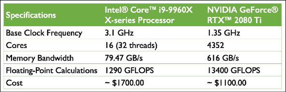
The sources for the information in the table are the following websites (Date: October 2019):

• https://ark.intel.com/content/www/us/en/ark/products/189123/intel-core-i9-9960x-x-series-processor-22m-cache-up-to-4-50-ghz.html
• https://www.nvidia.com/en-us/geforce/graphics-cards/rtx-2080-ti/

At 65 percent of the price of a modern CPU, we can get a GPU that has 272 times more cores and is capable of around 10 times more floating-point calculations per second. So, what is holding us back from utilizing GPUs for our machine learning tasks? The challenge is that writing code to target GPUs is not as simple as executing Python code in our interpreter. There are special packages, such as CUDA and OpenCL, that allow us to target the GPU. However, writing code in CUDA or OpenCL is probably not the most convenient environment for implementing and running machine learning algorithms. The good news is that this is what TensorFlow was developed for!

What is TensorFlow?

TensorFlow is a scalable and multiplatform programming interface for implementing and running machine learning algorithms, including convenience wrappers for deep learning. TensorFlow was developed by the researchers and engineers from the Google Brain team. While the main development is led by a team of researchers and software engineers at Google, its development also involves many contributions from the open source community. TensorFlow was initially built for internal use at Google, but it was subsequently released in November 2015 under a permissive open source license. Many machine learning researchers and practitioners from academia and industry have adapted TensorFlow to develop deep learning solutions.

To improve the performance of training machine learning models, TensorFlow allows execution on both CPUs and GPUs. However, its greatest performance capabilities can be discovered when using GPUs. TensorFlow supports CUDA-enabled GPUs officially. Support for OpenCL-enabled devices is still experimental. However, OpenCL will likely be officially supported in the near future. TensorFlow currently supports frontend interfaces for a number of programming languages.

Luckily for us as Python users, TensorFlow's Python API is currently the most complete API, thereby it attracts many machine learning and deep learning practitioners. Furthermore, TensorFlow has an official API in C++. In addition, new tools based on TensorFlow have been released, TensorFlow.js and TensorFlow Lite, that focus on running and deploying machine learning models in a web browser and on mobile and Internet of Things (IoT) devices. The APIs in other languages, such as Java, Haskell, Node.js, and Go, are not stable yet, but the open source community and TensorFlow developers are constantly improving them.

TensorFlow is built around a computation graph composed of a set of nodes. Each node represents an operation that may have zero or more input or output. A tensor is created as a symbolic handle to refer to the input and output of these operations.

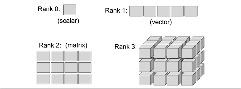
Mathematically, tensors can be understood as a generalization of scalars, vectors, matrices, and so on. More concretely, a scalar can be defined as a rank-0 tensor, a vector can be defined as a rank-1 tensor, a matrix can be defined as a rank-2 tensor, and matrices stacked in a third dimension can be defined as rank-3 tensors. But note that in TensorFlow, the values are stored in NumPy arrays, and the tensors provide references to these arrays.

To make the concept of a tensor clearer, consider the following figure, which represents tensors of ranks 0 and 1 in the first row, and tensors of ranks 2 and 3 in the second row:

In the original TensorFlow release, TensorFlow computations relied on constructing a static, directed graph to represent the data flow. As the use of static computation graphs proved to be a major friction point for many users, the TensorFlow library recently received a major overhaul with its 2.0 version, which makes building and training NN models a lot simpler. While TensorFlow 2.0 still supports static computation graphs, it now uses dynamic computation graphs, which allows for more flexibility.

How we will learn TensorFlow

First, we are going to cover TensorFlow's programming model, in particular, creating and manipulating tensors. Then, we will see how to load data and utilize TensorFlow Dataset objects, which will allow us to iterate through a dataset efficiently. In addition, we will discuss the existing, ready-to-use datasets in the tensorflow_datasets submodule and learn how to use them.

After learning about these basics, the tf.keras API will be introduced and we will move forward to building machine learning models, learn how to compile and train the models, and learn how to save the trained models on disk for future evaluation.

First steps with TensorFlow

In this section, we will take our first steps in using the low-level TensorFlow API. After installing TensorFlow, we will cover how to create tensors in TensorFlow and different ways of manipulating them, such as changing their shape, data type, and so on.

Installing TensorFlow

Depending on how your system is set up, you can typically just use Python's pip installer and install TensorFlow from PyPI by executing the following from your terminal:

pip install tensorflow

This will install the latest stable version, which is 2.0.0 at the time of writing. In order to ensure that the code presented in this chapter can be executed as expected, it is recommended that you use TensorFlow 2.0.0, which can be installed by specifying the version explicitly:

pip install tensorflow==[desired-version]

In case you want to use GPUs (recommended), you need a compatible NVIDIA graphics card, along with the CUDA Toolkit and the NVIDIA cuDNN library to be installed. If your machine satisfies these requirements, you can install TensorFlow with GPU support, as follows:

pip install tensorflow-gpu

For more information about the installation and setup process, please see the official recommendations at https://www.tensorflow.org/install/gpu.

Note that TensorFlow is still under active development; therefore, every couple of months, newer versions are released with significant changes. At the time of writing this chapter, the latest TensorFlow version is 2.0. You can verify your TensorFlow version from your terminal, as follows:

python -c 'import tensorflow as tf; print(tf.__version__)'

Creating tensors in TensorFlow

Now, let's consider a few different ways of creating tensors, and then see some of their properties and how to manipulate them. Firstly, we can simply create a tensor from a list or a NumPy array using the tf.convert_to_tensor function as follows:

>>> import tensorflow as tf
>>> import numpy as np
>>> np.set_printoptions(precision=3)
>>> a = np.array([1, 2, 3], dtype=np.int32)
>>> b = [4, 5, 6]
>>> t_a = tf.convert_to_tensor(a)
>>> t_b = tf.convert_to_tensor(b)
>>> print(t_a)
>>> print(t_b)
tf.Tensor([1 2 3], shape=(3,), dtype=int32)
tf.Tensor([4 5 6], shape=(3,), dtype=int32)

This resulted in tensors t_a and t_b, with their properties, shape=(3,) and dtype=int32, adopted from their source. Similar to NumPy arrays, we can further see these properties:

>>> t_ones = tf.ones((2, 3))
>>> t_ones.shape
TensorShape([2, 3])

To get access to the values that a tensor refers to, we can simply call the .numpy() method on a tensor:

>>> t_ones.numpy()
array([[1., 1., 1.],
       [1., 1., 1.]], dtype=float32)

Finally, creating a tensor of constant values can be done as follows:

>>> const_tensor = tf.constant([1.2, 5, np.pi],
...                            dtype=tf.float32)
>>> print(const_tensor)
tf.Tensor([1.2   5.    3.142], shape=(3,), dtype=float32)

Manipulating the data type and shape of a tensor

Learning ways to manipulate tensors is necessary to make them compatible for input to a model or an operation. In this section, you will learn how to manipulate tensor data types and shapes via several TensorFlow functions that cast, reshape, transpose, and squeeze.

The tf.cast() function can be used to change the data type of a tensor to a desired type:

>>> t_a_new = tf.cast(t_a, tf.int64)
>>> print(t_a_new.dtype)
<dtype: 'int64'>

As you will see in upcoming chapters, certain operations require that the input tensors have a certain number of dimensions (that is, rank) associated with a certain number of elements (shape). Thus, we might need to change the shape of a tensor, add a new dimension, or squeeze an unnecessary dimension. TensorFlow provides useful functions (or operations) to achieve this, such as tf.transpose(), tf.reshape(), and tf.squeeze(). Let's take a look at some examples:

• Transposing a tensor:

  >>> t = tf.random.uniform(shape=(3, 5))
  >>> t_tr = tf.transpose(t)
  >>> print(t.shape, ' --> ', t_tr.shape)
  (3, 5)  -->  (5, 3)
  

• Reshaping a tensor (for example, from a 1D vector to a 2D array):

  >>> t = tf.zeros((30,))
  >>> t_reshape = tf.reshape(t, shape=(5, 6))
  >>> print(t_reshape.shape)
  (5, 6)
  

• Removing the unnecessary dimensions (dimensions that have size 1, which are not needed):

  >>> t = tf.zeros((1, 2, 1, 4, 1))
  >>> t_sqz = tf.squeeze(t, axis=(2, 4))
  >>> print(t.shape, ' --> ', t_sqz.shape)
  (1, 2, 1, 4, 1)  -->  (1, 2, 4)
  

Applying mathematical operations to tensors

Applying mathematical operations, in particular linear algebra operations, is necessary for building most machine learning models. In this subsection, we will cover some widely used linear algebra operations, such as element-wise product, matrix multiplication, and computing the norm of a tensor.

First, let's instantiate two random tensors, one with uniform distribution in the range [–1, 1) and the other with a standard normal distribution:

>>> tf.random.set_seed(1)
>>> t1 = tf.random.uniform(shape=(5, 2),
...                        minval=-1.0, maxval=1.0)
>>> t2 = tf.random.normal(shape=(5, 2),
...                       mean=0.0, stddev=1.0)

Notice that t1 and t2 have the same shape. Now, to compute the element-wise product of t1 and t2, we can use the following:

>>> t3 = tf.multiply(t1, t2).numpy()
>>> print(t3)
[[-0.27  -0.874]
 [-0.017 -0.175]
 [-0.296 -0.139]
 [-0.727  0.135]
 [-0.401  0.004]]

To compute the mean, sum, and standard deviation along a certain axis (or axes), we can use tf.math.reduce_mean(), tf.math.reduce_sum(), and tf.math.reduce_std(). For example, the mean of each column in t1 can be computed as follows:

>>> t4 = tf.math.reduce_mean(t1, axis=0)
>>> print(t4)
tf.Tensor([0.09  0.207], shape=(2,), dtype=float32)

The matrix-matrix product between t1 and t2 (that is, , where the superscript T is for transpose) can be computed by using the tf.linalg.matmul() function as follows:

>>> t5 = tf.linalg.matmul(t1, t2, transpose_b=True)
>>> print(t5.numpy())
[[-1.144  1.115 -0.87  -0.321  0.856]
 [ 0.248 -0.191  0.25  -0.064 -0.331]
 [-0.478  0.407 -0.436  0.022  0.527]
 [ 0.525 -0.234  0.741 -0.593 -1.194]
 [-0.099  0.26   0.125 -0.462 -0.396]]

On the other hand, computing is performed by transposing t1, resulting in an array of size :

>>> t6 = tf.linalg.matmul(t1, t2, transpose_a=True)
>>> print(t6.numpy())
[[-1.711  0.302]
 [ 0.371 -1.049]]

Finally, the tf.norm() function is useful for computing the norm of a tensor. For example, we can calculate the norm of t1 as follows:

>>> norm_t1 = tf.norm(t1, ord=2, axis=1).numpy()
>>> print(norm_t1)
[1.046 0.293 0.504 0.96  0.383]

To verify that this code snippet computes the norm of t1 correctly, you can compare the results with the following NumPy function: np.sqrt(np.sum(np.square(t1), axis=1)).

Split, stack, and concatenate tensors

In this subsection, we will cover TensorFlow operations for splitting a tensor into multiple tensors, or the reverse: stacking and concatenating multiple tensors into a single one.

Assume that we have a single tensor and we want to split it into two or more tensors. For this, TensorFlow provides a convenient tf.split() function, which divides an input tensor into a list of equally-sized tensors. We can determine the desired number of splits as an integer using the argument num_or_size_splits to split a tensor along a desired dimension specified by the axis argument. In this case, the total size of the input tensor along the specified dimension must be divisible by the desired number of splits. Alternatively, we can provide the desired sizes in a list. Let's have a look at an example of both these options:

• Providing the number of splits (must be divisible):

  >>> tf.random.set_seed(1)
  >>> t = tf.random.uniform((6,))
  >>> print(t.numpy())
  [0.165 0.901 0.631 0.435 0.292 0.643]
  >>> t_splits = tf.split(t, num_or_size_splits=3)
  >>> [item.numpy() for item in t_splits]
  [array([0.165, 0.901], dtype=float32),
   array([0.631, 0.435], dtype=float32),
   array([0.292, 0.643], dtype=float32)]
  

  In this example, a tensor of size 6 was divided into a list of three tensors each with size 2.

• Providing the sizes of different splits:

  Alternatively, instead of defining the number of splits, we can also specify the sizes of the output tensors directly. Here, we are splitting a tensor of size 5 into tensors of sizes 3 and 2:

  >>> tf.random.set_seed(1)
  >>> t = tf.random.uniform((5,))
  >>> print(t.numpy())
  [0.165 0.901 0.631 0.435 0.292]
  >>> t_splits = tf.split(t, num_or_size_splits=[3, 2])
  >>> [item.numpy() for item in t_splits]
  [array([0.165, 0.901, 0.631], dtype=float32),
   array([0.435, 0.292], dtype=float32)]
  

Sometimes, we are working with multiple tensors and need to concatenate or stack them to create a single tensor. In this case, TensorFlow functions such as tf.stack() and tf.concat() come in handy. For example, let's create a 1D tensor, A, containing 1s with size 3 and a 1D tensor, B, containing 0s with size 2 and concatenate them into a 1D tensor, C, of size 5:

>>> A = tf.ones((3,))
>>> B = tf.zeros((2,))
>>> C = tf.concat([A, B], axis=0)
>>> print(C.numpy())
[1. 1. 1. 0. 0.]

If we create 1D tensors A and B, both with size 3, then we can stack them together to form a 2D tensor, S:

>>> A = tf.ones((3,))
>>> B = tf.zeros((3,))
>>> S = tf.stack([A, B], axis=1)
>>> print(S.numpy())
[[1. 0.]
 [1. 0.]
 [1. 0.]]

The TensorFlow API has many operations that you can use for building a model, processing your data, and more. However, covering every function is outside the scope of this book, where we will focus on the most essential ones. For the full list of operations and functions, you can refer to the documentation page of TensorFlow at https://www.tensorflow.org/versions/r2.0/api_docs/python/tf.

Building input pipelines using tf.data – the TensorFlow Dataset API

When we are training a deep NN model, we usually train the model incrementally using an iterative optimization algorithm such as stochastic gradient descent, as we have seen in previous chapters.

As mentioned at the beginning of this chapter, the Keras API is a wrapper around TensorFlow for building NN models. The Keras API provides a method, .fit(), for training the models. In cases where the training dataset is rather small and can be loaded as a tensor into the memory, TensorFlow models (that are built with the Keras API) can directly use this tensor via their .fit() method for training. In typical use cases, however, when the dataset is too large to fit into the computer memory, we will need to load the data from the main storage device (for example, the hard drive or solid-state drive) in chunks, that is, batch by batch (note the use of the term "batch" instead of "mini-batch" in this chapter to stay close to the TensorFlow terminology). In addition, we may need to construct a data-processing pipeline to apply certain transformations and preprocessing steps to our data, such as mean centering, scaling, or adding noise to augment the training procedure and to prevent overfitting.

Applying preprocessing functions manually every time can be quite cumbersome. Luckily, TensorFlow provides a special class for constructing efficient and convenient preprocessing pipelines. In this section, we will see an overview of different methods for constructing a TensorFlow Dataset, including dataset transformations and common preprocessing steps.

Creating a TensorFlow Dataset from existing tensors

If the data already exists in the form of a tensor object, a Python list, or a NumPy array, we can easily create a dataset using the tf.data.Dataset.from_tensor_slices() function. This function returns an object of class Dataset, which we can use to iterate through the individual elements in the input dataset. As a simple example, consider the following code, which creates a dataset from a list of values:

>>> a = [1.2, 3.4, 7.5, 4.1, 5.0, 1.0]
>>> ds = tf.data.Dataset.from_tensor_slices(a)
>>> print(ds)
<TensorSliceDataset shapes: (), types: tf.float32>

We can easily iterate through a dataset entry by entry as follows:

>>> for item in ds:
...     print(item)
tf.Tensor(1.2, shape=(), dtype=float32)
tf.Tensor(3.4, shape=(), dtype=float32)
tf.Tensor(7.5, shape=(), dtype=float32)
tf.Tensor(4.1, shape=(), dtype=float32)
tf.Tensor(5.0, shape=(), dtype=float32)
tf.Tensor(1.0, shape=(), dtype=float32)

If we want to create batches from this dataset, with a desired batch size of 3, we can do this as follows:

>>> ds_batch = ds.batch(3)
>>> for i, elem in enumerate(ds_batch, 1):
...    print('batch {}:'.format(i), elem.numpy())
batch 1: [1.2 3.4 7.5]
batch 2: [4.1 5.  1. ]

This will create two batches from this dataset, where the first three elements go into batch #1, and the remaining elements go into batch #2. The .batch() method has an optional argument, drop_remainder, which is useful for cases when the number of elements in the tensor is not divisible by the desired batch size. The default for drop_remainder is False. We will see more examples illustrating the behavior of this method later in the subsection Shuffle, batch, and repeat.

Combining two tensors into a joint dataset

Often, we may have the data in two (or possibly more) tensors. For example, we could have a tensor for features and a tensor for labels. In such cases, we need to build a dataset that combines these tensors together, which will allow us to retrieve the elements of these tensors in tuples.

Assume that we have two tensors, t_x and t_y. Tensor t_x holds our feature values, each of size 3, and t_y stores the class labels. For this example, we first create these two tensors as follows:

>>> tf.random.set_seed(1)
>>> t_x = tf.random.uniform([4, 3], dtype=tf.float32)
>>> t_y = tf.range(4)

Now, we want to create a joint dataset from these two tensors. Note that there is a required one-to-one correspondence between the elements of these two tensors:

>>> ds_x = tf.data.Dataset.from_tensor_slices(t_x)
>>> ds_y = tf.data.Dataset.from_tensor_slices(t_y)
>>>
>>> ds_joint = tf.data.Dataset.zip((ds_x, ds_y))
>>> for example in ds_joint:
...     print('  x:', example[0].numpy(),
...           '  y:', example[1].numpy())
  x: [0.165 0.901 0.631]   y: 0
  x: [0.435 0.292 0.643]   y: 1
  x: [0.976 0.435 0.66 ]   y: 2
  x: [0.605 0.637 0.614]   y: 3

Here, we first created two separate datasets, namely ds_x and ds_y. We then used the zip function to form a joint dataset. Alternatively, we can create the joint dataset using tf.data.Dataset.from_tensor_slices() as follows:

>>> ds_joint = tf.data.Dataset.from_tensor_slices((t_x, t_y))
>>> for example in ds_joint:
...     print('  x:', example[0].numpy(),
...           '  y:', example[1].numpy())
  x: [0.165 0.901 0.631]   y: 0
  x: [0.435 0.292 0.643]   y: 1
  x: [0.976 0.435 0.66 ]   y: 2
  x: [0.605 0.637 0.614]   y: 3

which results in the same output.

Note that a common source of error could be that the element-wise correspondence between the original features (x) and labels (y) might be lost (for example, if the two datasets are shuffled separately). However, once they are merged into one dataset, it is safe to apply these operations.

Next, we will see how to apply transformations to each individual element of a dataset. For this, we will use the previous ds_joint dataset and apply feature-scaling to scale the values to the range [-1, 1), as currently the values of t_x are in the range [0, 1) based on a random uniform distribution:

>>> ds_trans = ds_joint.map(lambda x, y: (x*2-1.0, y))
>>> for example in ds_trans:
...    print('  x:', example[0].numpy(),
...          '  y:', example[1].numpy())
  x: [-0.67   0.803  0.262]   y: 0
  x: [-0.131 -0.416  0.285]   y: 1
  x: [ 0.952 -0.13   0.32 ]   y: 2
  x: [ 0.21   0.273  0.229]   y: 3

Applying this sort of transformation can be used for a user-defined function. For example, if we have a dataset created from the list of image filenames on disk, we can define a function to load the images from these filenames and apply that function by calling the .map() method. You will see an example of applying multiple transformations to a dataset later in this chapter.

Shuffle, batch, and repeat

As was mentioned in Chapter 2, Training Simple Machine Learning Algorithms for Classification, to train an NN model using stochastic gradient descent optimization, it is important to feed training data as randomly shuffled batches. You have already seen how to create batches by calling the .batch() method of a dataset object. Now, in addition to creating batches, you will see how to shuffle and reiterate over the datasets. We will continue working with the previous ds_joint dataset.

First, let's create a shuffled version from the ds_joint dataset:

>>> tf.random.set_seed(1)
>>> ds = ds_joint.shuffle(buffer_size=len(t_x))
>>> for example in ds:
...     print('  x:', example[0].numpy(),
...           '  y:', example[1].numpy())
  x: [0.976 0.435 0.66 ]   y: 2
  x: [0.435 0.292 0.643]   y: 1
  x: [0.165 0.901 0.631]   y: 0
  x: [0.605 0.637 0.614]   y: 3

where the rows are shuffled without losing the one-to-one correspondence between the entries in x and y. The .shuffle() method requires an argument called buffer_size, which determines how many elements in the dataset are grouped together before shuffling. The elements in the buffer are randomly retrieved and their place in the buffer is given to the next elements in the original (unshuffled) dataset. Therefore, if we choose a small buffer_size, we may not shuffle the dataset perfectly.

If the dataset is small, choosing a relatively small buffer_size may negatively affect the predictive performance of the NN as the dataset may not be completely randomized. In practice, however, it usually does not have a noticeable effect when working with relatively large datasets, which is common in deep learning. Alternatively, to ensure complete randomization during each epoch, we can simply choose a buffer size that is equal to the number of the training examples, as in the preceding code (buffer_size=len(t_x)).

You will recall that dividing a dataset into batches for model training is done by calling the .batch() method. Now, let's create such batches from the ds_joint dataset and take a look at what a batch looks like:

>>> ds = ds_joint.batch(batch_size=3,
...                     drop_remainder=False)
>>> batch_x, batch_y = next(iter(ds))
>>> print('Batch-x:
', batch_x.numpy())
Batch-x:
[[0.165 0.901 0.631]
 [0.435 0.292 0.643]
 [0.976 0.435 0.66 ]]
>>> print('Batch-y: ', batch_y.numpy())
Batch-y: [0 1 2]

In addition, when training a model for multiple epochs, we need to shuffle and iterate over the dataset by the desired number of epochs. So, let's repeat the batched dataset twice:

>>> ds = ds_joint.batch(3).repeat(count=2)
>>> for i,(batch_x, batch_y) in enumerate(ds):
...     print(i, batch_x.shape, batch_y.numpy())
0 (3, 3) [0 1 2]
1 (1, 3) [3]
2 (3, 3) [0 1 2]
3 (1, 3) [3]

This results in two copies of each batch. If we change the order of these two operations, that is, first batch and then repeat, the results will be different:

>>> ds = ds_joint.repeat(count=2).batch(3)
>>> for i,(batch_x, batch_y) in enumerate(ds):
...     print(i, batch_x.shape, batch_y.numpy())
0 (3, 3) [0 1 2]
1 (3, 3) [3 0 1]
2 (2, 3) [2 3]

Notice the difference between the batches. When we first batch and then repeat, we get four batches. On the other hand, when repeat is performed first, three batches are created.

Finally, to get a better understanding of how these three operations (batch, shuffle, and repeat) behave, let's experiment with them in different orders. First, we will combine the operations in the following order: (1) shuffle, (2) batch, and (3) repeat:

## Order 1: shuffle -> batch -> repeat
>>> tf.random.set_seed(1)
>>> ds = ds_joint.shuffle(4).batch(2).repeat(3)
>>> for i,(batch_x, batch_y) in enumerate(ds):
...     print(i, batch_x.shape, batch_y.numpy())
0 (2, 3) [2 1]
1 (2, 3) [0 3]
2 (2, 3) [0 3]
3 (2, 3) [1 2]
4 (2, 3) [3 0]
5 (2, 3) [1 2]

Now, let's try a different order: (2) batch, (1) shuffle, and (3) repeat:

## Order 2: batch -> shuffle -> repeat
>>> tf.random.set_seed(1)
>>> ds = ds_joint.batch(2).shuffle(4).repeat(3)
>>> for i,(batch_x, batch_y) in enumerate(ds):
...     print(i, batch_x.shape, batch_y.numpy())
0 (2, 3) [0 1]
1 (2, 3) [2 3]
2 (2, 3) [0 1]
3 (2, 3) [2 3]
4 (2, 3) [2 3]
5 (2, 3) [0 1]

While the first code example (shuffle, batch, repeat) appears to have shuffled the dataset as expected, we can see that in the second case (batch, shuffle, repeat), the elements within a batch were not shuffled at all. We can observe this lack of shuffling by taking a closer look at the tensor containing the target values, y. All batches contain either the pair of values [y=0, y=1] or the remaining pair of values [y=2, y=3]; we do not observe the other possible permutations: [y=2, y=0], [y=1, y=3], and so forth. Note that in order to ensure these results are not coincidental, you may want to repeat this with a higher number than 3. For example, try it with .repeat(20).

Now, can you predict what will happen if we use the shuffle operation after repeat, for example, (2) batch, (3) repeat, (1) shuffle? Give it a try.

Creating a dataset from files on your local storage disk

In this section, we will build a dataset from image files stored on disk. There is an image folder associated with the online content of this chapter. After downloading the folder, you should be able to see six images of cats and dogs in JPEG format.

This small dataset will show how building a dataset from stored files generally works. To accomplish this, we are going to use two additional modules in TensorFlow: tf.io to read the image file contents, and tf.image to decode the raw contents and image resizing.

Before we start, let's take a look at the content of these files. We will use the pathlib library to generate a list of image files:

>>> import pathlib
>>> imgdir_path = pathlib.Path('cat_dog_images')
>>> file_list = sorted([str(path) for path in
...                     imgdir_path.glob('*.jpg')])
['cat_dog_images/dog-03.jpg', 'cat_dog_images/cat-01.jpg', 'cat_dog_images/cat-02.jpg', 'cat_dog_images/cat-03.jpg', 'cat_dog_images/dog-01.jpg', 'cat_dog_images/dog-02.jpg']

Next, we will visualize these image examples using Matplotlib:

>>> import matplotlib.pyplot as plt
>>> fig = plt.figure(figsize=(10, 5))
>>> for i, file in enumerate(file_list):
...     img_raw = tf.io.read_file(file)
...     img = tf.image.decode_image(img_raw)
...     print('Image shape: ', img.shape)
...     ax = fig.add_subplot(2, 3, i+1)
...     ax.set_xticks([]); ax.set_yticks([])
...     ax.imshow(img)
...     ax.set_title(os.path.basename(file), size=15)
>>> plt.tight_layout()
>>> plt.show()
Image shape:  (900, 1200, 3)
Image shape:  (900, 1200, 3)
Image shape:  (900, 1200, 3)
Image shape:  (900, 742, 3)
Image shape:  (800, 1200, 3)
Image shape:  (800, 1200, 3)

The following figure shows the example images:

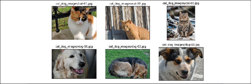
Just from this visualization and the printed image shapes, we can already see that the images have different aspect ratios. If you print the aspect ratios (or data array shapes) of these images, you will see that some images are 900 pixels high and 1200 pixels wide (), some are , and one is . Later, we will preprocess these images to a consistent size. Another point to consider is that the labels for these images are provided within their filenames. So, we extract these labels from the list of filenames, assigning label 1 to dogs and label 0 to cats:

>>> labels = [1 if 'dog' in os.path.basename(file) else 0
...           for file in file_list]
>>> print(labels)
[1, 0, 0, 0, 1, 1]

Now, we have two lists: a list of filenames (or paths of each image) and a list of their labels. In the previous section, you already learned two ways of creating a joint dataset from two tensors. Here, we will use the second approach as follows:

>>> ds_files_labels = tf.data.Dataset.from_tensor_slices(
...                                   (file_list, labels))
>>> for item in ds_files_labels:
...     print(item[0].numpy(), item[1].numpy())
b'cat_dog_images/dog-03.jpg' 1
b'cat_dog_images/cat-01.jpg' 0
b'cat_dog_images/cat-02.jpg' 0
b'cat_dog_images/cat-03.jpg' 0
b'cat_dog_images/dog-01.jpg' 1
b'cat_dog_images/dog-02.jpg' 1

We have called this dataset ds_files_labels, since it has filenames and labels. Next, we need to apply transformations to this dataset: load the image content from its file path, decode the raw content, and resize it to a desired size, for example, . Previously, we saw how to apply a lambda function using the .map() method. However, since we need to apply multiple preprocessing steps this time, we are going to write a helper function instead and use it when calling the .map() method:

>>> def load_and_preprocess(path, label):
...     image = tf.io.read_file(path)
...     image = tf.image.decode_jpeg(image, channels=3)
...     image = tf.image.resize(image, [img_height, img_width])
...     image /= 255.0
...     return image, label
>>> img_width, img_height = 120, 80
>>> ds_images_labels = ds_files_labels.map(load_and_preprocess)
>>>
>>> fig = plt.figure(figsize=(10, 6))
>>> for i,example in enumerate(ds_images_labels):
...     ax = fig.add_subplot(2, 3, i+1)
...     ax.set_xticks([]); ax.set_yticks([])
...     ax.imshow(example[0])
...     ax.set_title('{}'.format(example[1].numpy()),
...                  size=15)
>>> plt.tight_layout()
>>> plt.show()

This results in the following visualization of the retrieved example images, along with their labels:

The load_and_preprocess() function wraps all four steps into a single function, including the loading of the raw content, decoding it, and resizing the images. The function then returns a dataset that we can iterate over and apply other operations that we learned about in the previous sections.

Fetching available datasets from the tensorflow_datasets library

The tensorflow_datasets library provides a nice collection of freely available datasets for training or evaluating deep learning models. The datasets are nicely formatted and come with informative descriptions, including the format of features and labels and their type and dimensionality, as well as the citation of the original paper that introduced the dataset in BibTeX format. Another advantage is that these datasets are all prepared and ready to use as tf.data.Dataset objects, so all the functions we covered in the previous sections can be used directly. So, let's see how to use these datasets in action.

First, we need to install the tensorflow_datasets library via pip from the command line:

pip install tensorflow-datasets

Now, let's import this module and take a look at the list of available datasets:

>>> import tensorflow_datasets as tfds
>>> print(len(tfds.list_builders()))
101
>>> print(tfds.list_builders()[:5])
['abstract_reasoning', 'aflw2k3d', 'amazon_us_reviews', 'bair_robot_pushing_small', 'bigearthnet']

The preceding code indicates that there are currently 101 datasets available (101 datasets at the time of writing this chapter, but this number will likely increase)—we printed the first five datasets to the command line. There are two ways of fetching a dataset, which we will cover in the following paragraphs by fetching two different datasets: CelebA (celeb_a) and the MNIST digit dataset.

The first approach consists of three steps:

1. Calling the dataset builder function
2. Executing the download_and_prepare() method
3. Calling the as_dataset() method

Let's work with the first step for the CelebA dataset and print the associated description that is provided within the library:

>>> celeba_bldr = tfds.builder('celeb_a')
>>> print(celeba_bldr.info.features)
FeaturesDict({'image': Image(shape=(218, 178, 3), dtype=tf.uint8), 'landmarks': FeaturesDict({'lefteye_x': Tensor(shape=(), dtype=tf.int64), 'lefteye_y': Tensor(shape=(), dtype=tf.int64), 'righteye_x': Tensor(shape=(), dtype=tf.int64), 'righteye_y': ...
>>> print(celeba_bldr.info.features['image'])
Image(shape=(218, 178, 3), dtype=tf.uint8)
>>> print(celeba_bldr.info.features['attributes'].keys())
dict_keys(['5_o_Clock_Shadow', 'Arched_Eyebrows', ...
>>> print(celeba_bldr.info.citation)
@inproceedings{conf/iccv/LiuLWT15,
  added-at = {2018-10-09T00:00:00.000+0200},
  author = {Liu, Ziwei and Luo, Ping and Wang, Xiaogang and Tang, Xiaoou},
  biburl = {https://www.bibsonomy.org/bibtex/250e4959be61db325d2f02c1d8cd7bfbb/dblp},
  booktitle = {ICCV},
  crossref = {conf/iccv/2015},
  ee = {http://doi.ieeecomputersociety.org/10.1109/ICCV.2015.425},
  interhash = {3f735aaa11957e73914bbe2ca9d5e702},
  intrahash = {50e4959be61db325d2f02c1d8cd7bfbb},
  isbn = {978-1-4673-8391-2},
  keywords = {dblp},
  pages = {3730-3738},
  publisher = {IEEE Computer Society},
  timestamp = {2018-10-11T11:43:28.000+0200},
  title = {Deep Learning Face Attributes in the Wild.},
  url = {http://dblp.uni-trier.de/db/conf/iccv/iccv2015.html#LiuLWT15},
  year = 2015
}

This provides some useful information to understand the structure of this dataset. The features are stored as a dictionary with three keys: 'image', 'landmarks', and 'attributes'.

The 'image' entry refers to the face image of a celebrity; 'landmarks' refers to the dictionary of extracted facial points, such as the position of the eyes, nose, and so on; and 'attributes' is a dictionary of 40 facial attributes for the person in the image, like facial expression, makeup, hair properties, and so on.

Next, we will call the download_and_prepare() method. This will download the data and store it on disk in a designated folder for all TensorFlow Datasets. If you have already done this once, it will simply check whether the data is already downloaded so that it does not re-download it if it already exists in the designated location:

>>> celeba_bldr.download_and_prepare()

Next, we will instantiate the datasets as follows:

>>> datasets = celeba_bldr.as_dataset(shuffle_files=False)
>>> datasets.keys()
dict_keys(['test', 'train', 'validation'])

This dataset is already split into train, test, and validation datasets. In order to see what the image examples look like, we can execute the following code:

>>> ds_train = datasets['train']
>>> assert isinstance(ds_train, tf.data.Dataset)
>>> example = next(iter(ds_train))
>>> print(type(example))
<class 'dict'>
>>> print(example.keys())
dict_keys(['image', 'landmarks', 'attributes'])

Note that the elements of this dataset come in a dictionary. If we want to pass this dataset to a supervised deep learning model during training, we have to reformat it as a tuple of (features, label). For the label, we will use the 'Male' category from the attributes. We will do this by applying a transformation via map():

>>> ds_train = ds_train.map(lambda item:
...                (item['image'],
...                tf.cast(item['attributes']['Male'], tf.int32)))

Finally, let's batch the dataset and take a batch of 18 examples from it to visualize them with their labels:

>>> ds_train = ds_train.batch(18)
>>> images, labels = next(iter(ds_train))
>>> print(images.shape, labels)
(18, 218, 178, 3) tf.Tensor([0 0 0 1 1 1 0 1 1 0 1 1 0 1 0 1 1 1], shape=(18,), dtype=int32)
>>> fig = plt.figure(figsize=(12, 8))
>>> for i,(image,label) in enumerate(zip(images, labels)):
...     ax = fig.add_subplot(3, 6, i+1)
...     ax.set_xticks([]); ax.set_yticks([])
...     ax.imshow(image)
...     ax.set_title('{}'.format(label), size=15)
>>> plt.show()

The examples and their labels that are retrieved from ds_train are shown in the following figure:

This was all we needed to do to fetch and use the CelebA image dataset.

Next, we will proceed with the second approach for fetching a dataset from tensorflow_datasets. There is a wrapper function called load() that combines the three steps for fetching a dataset in one. Let's see how it can be used to fetch the MNIST digit dataset:

>>> mnist, mnist_info = tfds.load('mnist', with_info=True,
...                               shuffle_files=False)
>>> print(mnist_info)
tfds.core.DatasetInfo(
    name='mnist',
    version=1.0.0,
    description='The MNIST database of handwritten digits.',
    urls=['https://storage.googleapis.com/cvdf-datasets/mnist/'],
    features=FeaturesDict({
        'image': Image(shape=(28, 28, 1), dtype=tf.uint8),
        'label': ClassLabel(shape=(), dtype=tf.int64, num_classes=10)
    },
    total_num_examples=70000,
    splits={
        'test': <tfds.core.SplitInfo num_examples=10000>,
        'train': <tfds.core.SplitInfo num_examples=60000>
    },
    supervised_keys=('image', 'label'),
    citation="""
        @article{lecun2010mnist,
          title={MNIST handwritten digit database},
          author={LeCun, Yann and Cortes, Corinna and Burges, CJ},
          journal={ATT Labs [Online]. Availablist},
          volume={2},
          year={2010}
        }
        
    """,
    redistribution_info=,
)
>>> print(mnist.keys())
dict_keys(['test', 'train'])

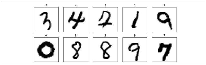
As we can see, the MNIST dataset is split into two partitions. Now, we can take the train partition, apply a transformation to convert the elements from a dictionary to a tuple, and visualize 10 examples:

>>> ds_train = mnist['train']
>>> ds_train = ds_train.map(lambda item:
...                         (item['image'], item['label']))
>>> ds_train = ds_train.batch(10)
>>> batch = next(iter(ds_train))
>>> print(batch[0].shape, batch[1])
(10, 28, 28, 1) tf.Tensor([8 4 7 7 0 9 0 3 3 3], shape=(10,), dtype=int64)
>>> fig = plt.figure(figsize=(15, 6))
>>> for i,(image,label) in enumerate(zip(batch[0], batch[1])):
...     ax = fig.add_subplot(2, 5, i+1)
...     ax.set_xticks([]); ax.set_yticks([])
...     ax.imshow(image[:, :, 0], cmap='gray_r')
...     ax.set_title('{}'.format(label), size=15)
>>> plt.show()

The retrieved example handwritten digits from this dataset are shown as follows:

This concludes our coverage of building and manipulating datasets and fetching datasets from the tensorflow_datasets library. Next, we will see how to build NN models in TensorFlow.

Building an NN model in TensorFlow

So far in this chapter, you have learned about the basic utility components of TensorFlow for manipulating tensors and organizing data into formats that we can iterate over during training. In this section, we will finally implement our first predictive model in TensorFlow. As TensorFlow is a bit more flexible but also more complex than machine learning libraries such as scikit-learn, we will start with a simple linear regression model.

The TensorFlow Keras API (tf.keras)

Keras is a high-level NN API and was originally developed to run on top of other libraries such as TensorFlow and Theano. Keras provides a user-friendly and modular programming interface that allows easy prototyping and the building of complex models in just a few lines of code. Keras can be installed independently from PyPI and then configured to use TensorFlow as its backend engine. Keras is tightly integrated into TensorFlow and its modules are accessible through tf.keras. In TensorFlow 2.0, tf.keras has become the primary and recommended approach for implementing models. This has the advantage that it supports TensorFlow-specific functionalities, such as dataset pipelines using tf.data, which you learned about in the previous section. In this book, we will use the tf.keras module to build NN models.

As you will see in the following subsections, the Keras API (tf.keras) makes building an NN model extremely easy. The most commonly used approach for building an NN in TensorFlow is through tf.keras.Sequential(), which allows stacking layers to form a network. A stack of layers can be given in a Python list to a model defined as tf.keras.Sequential(). Alternatively, the layers can be added one by one using the .add() method.

Furthermore, tf.keras allows us to define a model by subclassing tf.keras.Model. This gives us more control over the forward pass by defining the call() method for our model class to specify the forward pass explicitly. We will see examples of both of these approaches for building an NN model using the tf.keras API.

Finally, as you will see in the following subsections, models built using the tf.keras API can be compiled and trained via the .compile() and .fit() methods.

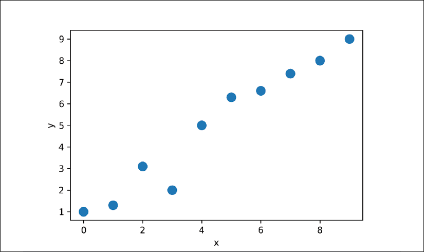
Building a linear regression model

In this subsection, we will build a simple model to solve a linear regression problem. First, let's create a toy dataset in NumPy and visualize it:

>>> X_train = np.arange(10).reshape((10, 1))
>>> y_train = np.array([1.0, 1.3, 3.1, 2.0, 5.0, 6.3,
...                     6.6, 7.4, 8.0, 9.0])
>>> plt.plot(X_train, y_train, 'o', markersize=10)
>>> plt.xlabel('x')
>>> plt.ylabel('y')
>>> plt.show()

As a result, the training examples will be shown in a scatterplot as follows:

Next, we will standardize the features (mean centering and dividing by the standard deviation) and create a TensorFlow Dataset:

>>> X_train_norm = (X_train - np.mean(X_train))/np.std(X_train)
>>> ds_train_orig = tf.data.Dataset.from_tensor_slices(
...                   (tf.cast(X_train_norm, tf.float32),
...                    tf.cast(y_train, tf.float32)))

Now, we can define our model for linear regression as . Here, we are going to use the Keras API. tf.keras provides predefined layers for building complex NN models, but to start, you will learn how to define a model from scratch. Later in this chapter, you will see how to use those predefined layers.

For this regression problem, we will define a new class derived from the tf.keras.Model class. Subclassing tf.keras.Model allows us to use the Keras tools for exploring a model, training, and evaluation. In the constructor of our class, we will define the parameters of our model, w and b, which correspond to the weight and the bias parameters, respectively. Finally, we will define the call() method to determine how this model uses the input data to generate its output:

>>> class MyModel(tf.keras.Model):
...     def __init__(self):
...         super(MyModel, self).__init__()
...         self.w = tf.Variable(0.0, name='weight')
...         self.b = tf.Variable(0.0, name='bias')
...
...     def call(self, x):
...         return self.w * x + self.b

Next, we will instantiate a new model from the MyModel() class that we can train based on the training data. The TensorFlow Keras API provides a method named .summary() for models that are instantiated from tf.keras.Model, which allows us to get a summary of the model components layer by layer and the number of parameters in each layer. Since we have sub-classed our model from tf.keras.Model, the .summary() method is also available to us. But, in order to be able to call model.summary(), we first need to specify the dimensionality of the input (the number of features) to this model. We can do this by calling model.build() with the expected shape of the input data:

>>> model = MyModel()
>>> model.build(input_shape=(None, 1))
>>> model.summary()
Model: "my_model"
_________________________________________________________________
Layer (type)                 Output Shape              Param #   
=================================================================
Total params: 2
Trainable params: 2
Non-trainable params: 0
_________________________________________________________________

Note that we used None as a placeholder for the first dimension of the expected input tensor via model.build(), which allows us to use an arbitrary batch size. However, the number of features is fixed (here 1) as it directly corresponds to the number of weight parameters of the model. Building model layers and parameters after instantiation by calling the .build() method is called late variable creation. For this simple model, we already created the model parameters in the constructor; therefore, specifying the input_shape via build() has no further effect on our parameters, but still it is needed if we want to call model.summary().

After defining the model, we can define the cost function that we want to minimize to find the optimal model weights. Here, we will choose the mean squared error (MSE) as our cost function. Furthermore, to learn the weight parameters of the model, we will use stochastic gradient descent. In this subsection, we will implement this training via the stochastic gradient descent procedure by ourselves, but in the next subsection, we will use the Keras methods compile() and fit() to do the same thing.

To implement the stochastic gradient descent algorithm, we need to compute the gradients. Rather than manually computing the gradients, we will use the TensorFlow API tf.GradientTape. We will cover tf.GradientTape and its different behaviors in Chapter 14, Going Deeper – The Mechanics of TensorFlow. The code is as follows:

>>> def loss_fn(y_true, y_pred):
...     return tf.reduce_mean(tf.square(y_true - y_pred))
>>> def train(model, inputs, outputs, learning_rate):
...     with tf.GradientTape() as tape:
...         current_loss = loss_fn(model(inputs), outputs)
...     dW, db = tape.gradient(current_loss, [model.w, model.b])
...     model.w.assign_sub(learning_rate * dW)
...     model.b.assign_sub(learning_rate * db)

Now, we can set the hyperparameters and train the model for 200 epochs. We will create a batched version of the dataset and repeat the dataset with count=None, which will result in an infinitely repeated dataset:

>>> tf.random.set_seed(1)
>>> num_epochs = 200
>>> log_steps = 100
>>> learning_rate = 0.001
>>> batch_size = 1
>>> steps_per_epoch = int(np.ceil(len(y_train) / batch_size))
>>> ds_train = ds_train_orig.shuffle(buffer_size=len(y_train))
>>> ds_train = ds_train.repeat(count=None)
>>> ds_train = ds_train.batch(1)
>>> Ws, bs = [], []
>>> for i, batch in enumerate(ds_train):
...     if i >= steps_per_epoch * num_epochs:
...         # break the infinite loop
...         break
...     Ws.append(model.w.numpy())
...     bs.append(model.b.numpy())
...
...     bx, by = batch
...     loss_val = loss_fn(model(bx), by)
...
...     train(model, bx, by, learning_rate=learning_rate)
...     if i%log_steps==0:
...         print('Epoch {:4d} Step {:2d} Loss {:6.4f}'.format(
...               int(i/steps_per_epoch), i, loss_val))
Epoch    0 Step  0 Loss 43.5600
Epoch   10 Step 100 Loss 0.7530
Epoch   20 Step 200 Loss 20.1759
Epoch   30 Step 300 Loss 23.3976
Epoch   40 Step 400 Loss 6.3481
Epoch   50 Step 500 Loss 4.6356
Epoch   60 Step 600 Loss 0.2411
Epoch   70 Step 700 Loss 0.2036
Epoch   80 Step 800 Loss 3.8177
Epoch   90 Step 900 Loss 0.9416
Epoch  100 Step 1000 Loss 0.7035
Epoch  110 Step 1100 Loss 0.0348
Epoch  120 Step 1200 Loss 0.5404
Epoch  130 Step 1300 Loss 0.1170
Epoch  140 Step 1400 Loss 0.1195
Epoch  150 Step 1500 Loss 0.0944
Epoch  160 Step 1600 Loss 0.4670
Epoch  170 Step 1700 Loss 2.0695
Epoch  180 Step 1800 Loss 0.0020
Epoch  190 Step 1900 Loss 0.3612

Let's look at the trained model and plot it. For test data, we will create a NumPy array of values evenly spaced between 0 to 9. Since we trained our model with standardized features, we will also apply the same standardization to the test data:

>>> print('Final Parameters: ', model.w.numpy(), model.b.numpy())
Final Parameters:  2.6576622 4.8798566
>>> X_test = np.linspace(0, 9, num=100).reshape(-1, 1)
>>> X_test_norm = (X_test - np.mean(X_train)) / np.std(X_train)
>>> y_pred = model(tf.cast(X_test_norm, dtype=tf.float32))
>>> fig = plt.figure(figsize=(13, 5))
>>> ax = fig.add_subplot(1, 2, 1)
>>> plt.plot(X_train_norm, y_train, 'o', markersize=10)
>>> plt.plot(X_test_norm, y_pred, '--', lw=3)
>>> plt.legend(['Training examples', 'Linear Reg.'], fontsize=15)
>>> ax.set_xlabel('x', size=15)
>>> ax.set_ylabel('y', size=15)
>>> ax.tick_params(axis='both', which='major', labelsize=15)
>>> ax = fig.add_subplot(1, 2, 2)
>>> plt.plot(Ws, lw=3)
>>> plt.plot(bs, lw=3)
>>> plt.legend(['Weight w', 'Bias unit b'], fontsize=15)
>>> ax.set_xlabel('Iteration', size=15)
>>> ax.set_ylabel('Value', size=15)
>>> ax.tick_params(axis='both', which='major', labelsize=15)
>>> plt.show()

The following figure shows the scatterplot of the training examples and the trained linear regression model, as well as the convergence history of the weight, w, and the bias unit, b:

Model training via the .compile() and .fit() methods

In the previous example, we saw how to train a model by writing a custom function, train(), and applied stochastic gradient descent optimization. However, writing the train() function can be a repeatable task across different projects. The TensorFlow Keras API provides a convenient .fit() method that can be called on an instantiated model. To show how this works, let's create a new model and compile it by selecting the optimizer, loss function, and evaluation metrics:

>>> tf.random.set_seed(1)
>>> model = MyModel()
>>> model.compile(optimizer='sgd',
...               loss=loss_fn,
...               metrics=['mae', 'mse'])

Now, we can simply call the fit() method to train the model. We can pass a batched dataset (like ds_train, which was created in the previous example). However, this time you will see that we can pass the NumPy arrays for x and y directly, without needing to create a dataset:

>>> model.fit(X_train_norm, y_train,
...           epochs=num_epochs, batch_size=batch_size,
...           verbose=1)
Train on 10 samples
Epoch 1/200
10/10 [==============================] - 0s 4ms/sample - loss: 27.8578 - mae: 4.5810 - mse: 27.8578
Epoch 2/200
10/10 [==============================] - 0s 738us/sample - loss: 18.6640 - mae: 3.7395 - mse: 18.6640
...
Epoch 200/200
10/10 [==============================] - 0s 1ms/sample - loss: 0.4139 - mae: 0.4942 - mse: 0.4139

After the model is trained, visualize the results and make sure that they are similar to the results of the previous method.

Building a multilayer perceptron for classifying flowers in the Iris dataset

In the previous example, you saw how to build a model from scratch. We trained this model using stochastic gradient descent optimization. While we started our journey based on the simplest possible example, you can see that defining the model from scratch, even for such a simple case, is neither appealing nor a good practice. TensorFlow instead provides already defined layers through tf.keras.layers that can be readily used as the building blocks of an NN model. In this section, you will learn how to use these layers to solve a classification task using the Iris flower dataset and build a two-layer perceptron using the Keras API. First, let's get the data from tensorflow_datasets:

>>> iris, iris_info = tfds.load('iris', with_info=True)
>>> print(iris_info)

This prints some information about this dataset (not printed here to save space). However, you will notice in the shown information that this dataset comes with only one partition, so we have to split the dataset into training and testing partitions (and validation for proper machine learning practice) on our own. Let's assume that we want to use two-thirds of the dataset for training and keep the remaining examples for testing. The tensorflow_datasets library provides a convenient tool that allows us to determine slices and splits via the DatasetBuilder object prior to loading a dataset. You can find out more about splits at https://www.tensorflow.org/datasets/splits.

An alternative approach is to load the entire dataset first and then use .take() and .skip() to split the dataset to two partitions. If the dataset is not shuffled at first, we can also shuffle the dataset. However, we need to be very careful with this because it can lead to mixing the train/test examples, which is not acceptable in machine learning. To avoid this, we have to set an argument, reshuffle_each_iteration=False, in the .shuffle() method. The code for splitting the dataset into train/test is as follows:

>>> tf.random.set_seed(1)
>>> ds_orig = iris['train']
>>> ds_orig = ds_orig.shuffle(150, reshuffle_each_iteration=False)
>>> ds_train_orig = ds_orig.take(100)
>>> ds_test = ds_orig.skip(100)

Next, as you have already seen in the previous sections, we need to apply a transformation via the .map() method to convert the dictionary to a tuple:

>>> ds_train_orig = ds_train_orig.map(
...     lambda x: (x['features'], x['label']))
>>> ds_test = ds_test.map(
...     lambda x: (x['features'], x['label']))

Now, we are ready to use the Keras API to build a model efficiently. In particular, using the tf.keras.Sequential class, we can stack a few Keras layers and build an NN. You can see the list of all the Keras layers that are already available at https://www.tensorflow.org/versions/r2.0/api_docs/python/tf/keras/layers. For this problem, we are going to use the Dense layer (tf.keras.layers.Dense), which is also known as a fully connected (FC) layer or linear layer, and can be best represented by , where x is the input features, w and b are the weight matrix and the bias vector, and f is the activation function.

If you think of the layers in an NN, each layer receives its inputs from the preceding layer; therefore, its dimensionality (rank and shape) is fixed. Typically, we need to concern ourselves with the dimensionality of output only when we design an NN architecture. (Note: the first layer is the exception, but TensorFlow/Keras allows us to decide the input dimensionality of the first layer after defining the model through late variable creation.) Here, we want to define a model with two hidden layers. The first one receives an input of four features and projects them to 16 neurons. The second layer receives the output of the previous layer (which has size 16) and projects them to three output neurons, since we have three class labels. This can be done using the Sequential class and the Dense layer in Keras as follows:

>>> iris_model = tf.keras.Sequential([
...         tf.keras.layers.Dense(16, activation='sigmoid',
...                               name='fc1', input_shape=(4,)),
...         tf.keras.layers.Dense(3, name='fc2',
...                               activation='softmax')])
>>> iris_model.summary()
Model: "sequential"
_________________________________________________________________
Layer (type)                 Output Shape              Param #   
=================================================================
fc1 (Dense)                  (None, 16)                80        
_________________________________________________________________
fc2 (Dense)                  (None, 3)                 51        
=================================================================
Total params: 131
Trainable params: 131
Non-trainable params: 0
_________________________________________________________________

Notice that we determined the input shape for the first layer via input_shape=(4,), and therefore, we did not have to call .build() anymore in order to use iris_model.summary().

The printed model summary indicates that the first layer (fc1) has 80 parameters, and the second layer has 51 parameters. You can verify that by , where is the number of input units, and is the number of output units. Recall that for a fully (densely) connected layer, the learnable parameters are the weight matrix of size and the bias vector of size . Furthermore, notice that we used the sigmoid activation function for the first layer and softmax activation for the last (output) layer. Softmax activation in the last layer is used to support multi-class classification, since here we have three class labels (which is why we have three neurons at the output layer). We will discuss the different activation functions and their applications later in this chapter.

Next, we will compile this model to specify the loss function, the optimizer, and the metrics for evaluation:

>>> iris_model.compile(optimizer='adam',
...                    loss='sparse_categorical_crossentropy',
...                    metrics=['accuracy'])

Now, we can train the model. We will specify the number of epochs to be 100 and the batch size to be 2. In the following code, we will build an infinitely repeating dataset, which will be passed to the fit() method for training the model. In this case, in order for the fit() method to be able to keep track of the epochs, it needs to know the number of steps for each epoch.

Given the size of our training data (here, 100) and the batch size (batch_size), we can determine the number of steps in each epoch, steps_per_epoch:

>>> num_epochs = 100
>>> training_size = 100
>>> batch_size = 2
>>> steps_per_epoch = np.ceil(training_size / batch_size)
>>> ds_train = ds_train_orig.shuffle(buffer_size=training_size)
>>> ds_train = ds_train.repeat()
>>> ds_train = ds_train.batch(batch_size=batch_size)
>>> ds_train = ds_train.prefetch(buffer_size=1000)
>>> history = iris_model.fit(ds_train, epochs=num_epochs,
...                          steps_per_epoch=steps_per_epoch,
...                          verbose=0)

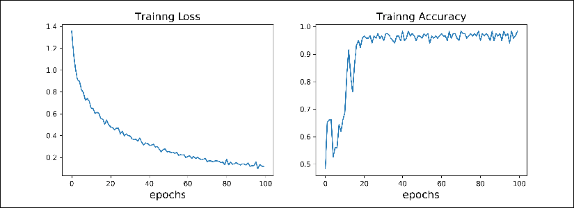
The returned variable history keeps the training loss and the training accuracy (since they were specified as metrics to iris_model.compile()) after each epoch. We can use this to visualize the learning curves as follows:

>>> hist = history.history
>>> fig = plt.figure(figsize=(12, 5))
>>> ax = fig.add_subplot(1, 2, 1)
>>> ax.plot(hist['loss'], lw=3)
>>> ax.set_title('Training loss', size=15)
>>> ax.set_xlabel('Epoch', size=15)
>>> ax.tick_params(axis='both', which='major', labelsize=15)
>>> ax = fig.add_subplot(1, 2, 2)
>>> ax.plot(hist['accuracy'], lw=3)
>>> ax.set_title('Training accuracy', size=15)
>>> ax.set_xlabel('Epoch', size=15)
>>> ax.tick_params(axis='both', which='major', labelsize=15)
>>> plt.show()

The learning curves (training loss and training accuracy) are as follows:

Evaluating the trained model on the test dataset

Since we specified 'accuracy' as our evaluation metric in iris_model.compile(), we can now directly evaluate the model on the test dataset:

>>> results = iris_model.evaluate(ds_test.batch(50), verbose=0)
>>> print('Test loss: {:.4f}   Test Acc.: {:.4f}'.format(*results))
Test loss: 0.0692   Test Acc.: 0.9800

Notice that we have to batch the test dataset as well, to ensure that the input to the model has the correct dimension (rank). As we discussed earlier, calling .batch() will increase the rank of the retrieved tensors by 1. The input data for .evaluate() must have one designated dimension for the batch, although here (for evaluation), the size of the batch does not matter. Therefore, if we pass ds_batch.batch(50) to the .evaluate() method, the entire test dataset will be processed in one batch of size 50, but if we pass ds_batch.batch(1), 50 batches of size 1 will be processed.

Saving and reloading the trained model

Trained models can be saved on disk for future use. This can be done as follows:

>>> iris_model.save('iris-classifier.h5',
...            overwrite=True,
...            include_optimizer=True,
...            save_format='h5')

The first option is the filename. Calling iris_model.save() will save both the model architecture and all the learned parameters. However, if you want to save only the architecture, you can use the iris_model.to_json() method, which saves the model configuration in JSON format. Or if you want to save only the model weights, you can do that by calling iris_model.save_weights(). The save_format can be specified to be either 'h5' for the HDF5 format or 'tf' for TensorFlow format.

Now, let's reload the saved model. Since we have saved both the model architecture and the weights, we can easily rebuild and reload the parameters in just one line:

>>> iris_model_new = tf.keras.models.load_model('iris-classifier.h5')

Try to verify the model architecture by calling iris_model_new.summary().

Finally, let's evaluate this new model that is reloaded on the test dataset to verify that the results are the same as before:

>>> results = iris_model_new.evaluate(ds_test.batch(33), verbose=0)
>>> print('Test loss: {:.4f}   Test Acc.: {:.4f}'.format(*results))
Test loss: 0.0692   Test Acc.: 0.9800

Choosing activation functions for multilayer neural networks

For simplicity, we have only discussed the sigmoid activation function in the context of multilayer feedforward NNs so far; we used it in the hidden layer as well as the output layer in the MLP implementation in Chapter 12, Implementing a Multilayer Artificial Neural Network from Scratch.

Note that in this book, the sigmoidal logistic function, , is referred to as the sigmoid function for brevity, which is common in machine learning literature. In the following subsections, you will learn more about alternative nonlinear functions that are useful for implementing multilayer NNs.

Technically, we can use any function as an activation function in multilayer NNs as long as it is differentiable. We can even use linear activation functions, such as in Adaline (Chapter 2, Training Simple Machine Learning Algorithms for Classification). However, in practice, it would not be very useful to use linear activation functions for both hidden and output layers, since we want to introduce nonlinearity in a typical artificial NN to be able to tackle complex problems. The sum of linear functions yields a linear function after all.

The logistic (sigmoid) activation function that we used in Chapter 12 probably mimics the concept of a neuron in a brain most closely—we can think of it as the probability of whether a neuron fires. However, the logistic (sigmoid) activation function can be problematic if we have highly negative input, since the output of the sigmoid function will be close to zero in this case. If the sigmoid function returns output that is close to zero, the NN will learn very slowly, and it will be more likely to get trapped in the local minima during training. This is why people often prefer a hyperbolic tangent as an activation function in hidden layers.

Before we discuss what a hyperbolic tangent looks like, let’s briefly recapitulate some of the basics of the logistic function and look at a generalization that makes it more useful for multilabel classification problems.

Logistic function recap

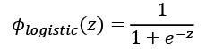
As was mentioned in the introduction to this section, the logistic function is, in fact, a special case of a sigmoid function. You will recall from the section on logistic regression in Chapter 3, A Tour of Machine Learning Classifiers Using scikit-learn, that we can use a logistic function to model the probability that sample x belongs to the positive class (class 1) in a binary classification task.

The given net input, z, is shown in the following equation:

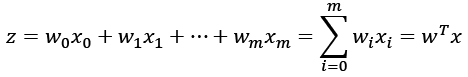
The logistic (sigmoid) function will compute the following:

Note that is the bias unit (y-axis intercept, which means ). To provide a more concrete example, let’s take a model for a two-dimensional data point, x, and a model with the following weight coefficients assigned to the w vector:

>>> import numpy as np
>>> X = np.array([1, 1.4, 2.5]) ## first value must be 1
>>> w = np.array([0.4, 0.3, 0.5])
>>> def net_input(X, w):
...     return np.dot(X, w)
>>> def logistic(z):
...     return 1.0 / (1.0 + np.exp(-z))
>>> def logistic_activation(X, w):
...     z = net_input(X, w)
...     return logistic(z)
>>> print(‘P(y=1|x) = %.3f’ % logistic_activation(X, w))
P(y=1|x) = 0.888

If we calculate the net input (z) and use it to activate a logistic neuron with those particular feature values and weight coefficients, we get a value of 0.888, which we can interpret as an 88.8 percent probability that this particular sample, x, belongs to the positive class.

In Chapter 12, we used the one-hot encoding technique to represent multiclass ground truth labels and designed the output layer consisting of multiple logistic activation units. However, as will be demonstrated by the following code example, an output layer consisting of multiple logistic activation units does not produce meaningful, interpretable probability values:

>>> # W : array with shape = (n_output_units, n_hidden_units+1)
>>> #     note that the first column are the bias units
>>> W = np.array([[1.1, 1.2, 0.8, 0.4],
...               [0.2, 0.4, 1.0, 0.2],
...               [0.6, 1.5, 1.2, 0.7]])
>>> # A : data array with shape = (n_hidden_units + 1, n_samples)
>>> #     note that the first column of this array must be 1
>>> A = np.array([[1, 0.1, 0.4, 0.6]])
>>> Z = np.dot(W, A[0])
>>> y_probas = logistic(Z)
>>> print(‘Net Input: 
’, Z)
Net Input:
[ 1.78  0.76  1.65]
>>> print(‘Output Units:
’, y_probas)
Output Units:
[ 0.85569687  0.68135373  0.83889105]

As you can see in the output, the resulting values cannot be interpreted as probabilities for a three-class problem. The reason for this is that they do not sum up to 1. However, this is, in fact, not a big concern if we use our model to predict only the class labels and not the class membership probabilities. One way to predict the class label from the output units obtained earlier is to use the maximum value:

>>> y_class = np.argmax(Z, axis=0)
>>> print(‘Predicted class label: %d’ % y_class)
Predicted class label: 0

In certain contexts, it can be useful to compute meaningful class probabilities for multiclass predictions. In the next section, we will take a look at a generalization of the logistic function, the softmax function, which can help us with this task.

Estimating class probabilities in multiclass classification via the softmax function

In the previous section, you saw how we can obtain a class label using the argmax function. Previously, in the section Building a multilayer perceptron for classifying flowers in the Iris dataset, we determined activation=’softmax’ in the last layer of the MLP model. The softmax function is a soft form of the argmax function; instead of giving a single class index, it provides the probability of each class. Therefore, it allows us to compute meaningful class probabilities in multiclass settings (multinomial logistic regression).

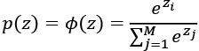
In softmax, the probability of a particular sample with net input z belonging to the ith class can be computed with a normalization term in the denominator, that is, the sum of the exponentially weighted linear functions:

To see softmax in action, let’s code it up in Python:

>>> def softmax(z):
...     return np.exp(z) / np.sum(np.exp(z))
>>> y_probas = softmax(Z)
>>> print(‘Probabilities:
’, y_probas)
Probabilities:
[ 0.44668973  0.16107406  0.39223621]
>>> np.sum(y_probas)
1.0

As you can see, the predicted class probabilities now sum up to 1, as we would expect. It is also notable that the predicted class label is the same as when we applied the argmax function to the logistic output.

It may help to think of the result of the softmax function as a normalized output that is useful for obtaining meaningful class-membership predictions in multiclass settings. Therefore, when we build a multiclass classification model in TensorFlow, we can use the tf.keras.activations.softmax() function to estimate the probabilities of each class membership for an input batch of examples. To see how we can use the softmax activation function in TensorFlow, in the following code, we will convert Z to a tensor, with an additional dimension reserved for the batch size:

>>> import tensorflow as tf
>>> Z_tensor = tf.expand_dims(Z, axis=0)
>>> tf.keras.activations.softmax(Z_tensor)
<tf.Tensor: id=21, shape=(1, 3), dtype=float64, numpy=array([[0.44668973, 0.16107406, 0.39223621]])>

Broadening the output spectrum using a hyperbolic tangent

Another sigmoidal function that is often used in the hidden layers of artificial NNs is the hyperbolic tangent (commonly known as tanh), which can be interpreted as a rescaled version of the logistic function:

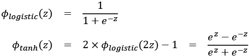
The advantage of the hyperbolic tangent over the logistic function is that it has a broader output spectrum ranging in the open interval (–1, 1), which can improve the convergence of the back-propagation algorithm (Neural Networks for Pattern Recognition, C. M. Bishop, Oxford University Press, pages: 500-501, 1995).

In contrast, the logistic function returns an output signal ranging in the open interval (0, 1). For a simple comparison of the logistic function and the hyperbolic tangent, let’s plot the two sigmoidal functions:

>>> import matplotlib.pyplot as plt
>>> def tanh(z):
...     e_p = np.exp(z)
...     e_m = np.exp(-z)
...     return (e_p - e_m) / (e_p + e_m)
>>> z = np.arange(-5, 5, 0.005)
>>> log_act = logistic(z)
>>> tanh_act = tanh(z)
>>> plt.ylim([-1.5, 1.5])
>>> plt.xlabel(‘net input $z$’)
>>> plt.ylabel(‘activation $phi(z)$’)
>>> plt.axhline(1, color=’black’, linestyle=’:’)
>>> plt.axhline(0.5, color=’black’, linestyle=’:’)
>>> plt.axhline(0, color=’black’, linestyle=’:’)
>>> plt.axhline(-0.5, color=’black’, linestyle=’:’)
>>> plt.axhline(-1, color=’black’, linestyle=’:’)
>>> plt.plot(z, tanh_act,
...          linewidth=3, linestyle=’--’,
...          label=’tanh’)
>>> plt.plot(z, log_act,
...          linewidth=3,
...          label=’logistic’)
>>> plt.legend(loc=’lower right’)
>>> plt.tight_layout()
>>> plt.show()

As you can see, the shapes of the two sigmoidal curves look very similar; however, the tanh function has double the output space of the logistic function:

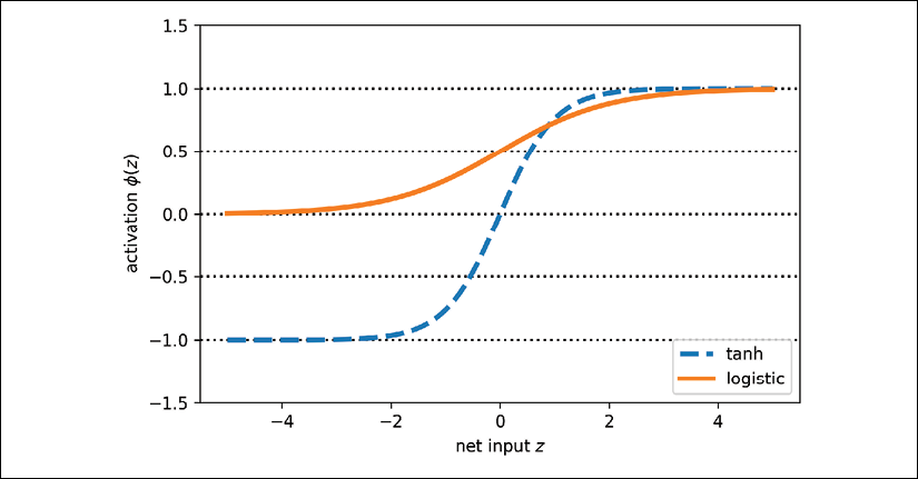
Note that we previously implemented the logistic and tanh functions verbosely for the purpose of illustration. In practice, we can use NumPy’s tanh function.

Alternatively, when building an NN model, we can use tf.keras.activations.tanh() in TensorFlow to achieve the same results:

>>> np.tanh(z)
array([-0.9999092 , -0.99990829, -0.99990737, ...,  0.99990644,
        0.99990737,  0.99990829])
>>> tf.keras.activations.tanh(z)
<tf.Tensor: id=14, shape=(2000,), dtype=float64, numpy=
array([-0.9999092 , -0.99990829, -0.99990737, ...,  0.99990644,
        0.99990737,  0.99990829])>

In addition, the logistic function is available in SciPy’s special module:

>>> from scipy.special import expit
>>> expit(z)
array([0.00669285, 0.00672617, 0.00675966, ..., 0.99320669, 0.99324034,
       0.99327383])

Similarly, we can use the tf.keras.activations.sigmoid() function in TensorFlow to do the same computation, as follows:

>>> tf.keras.activations.sigmoid(z)
<tf.Tensor: id=16, shape=(2000,), dtype=float64, numpy=
array([0.00669285, 0.00672617, 0.00675966, ..., 0.99320669, 0.99324034,
       0.99327383])>

Rectified linear unit activation

Rectified linear unit (ReLU) is another activation function that is often used in deep NNs. Before we delve into ReLU, we should step back and understand the vanishing gradient problem of tanh and logistic activations.

To understand this problem, let’s assume that we initially have the net input , which changes to . Computing the tanh activation, we get and , which shows no change in the output (due to the asymptotic behavior of the tanh function and numerical errors).

This means that the derivative of activations with respect to the net input diminishes as z becomes large. As a result, learning weights during the training phase becomes very slow because the gradient terms may be very close to zero. ReLU activation addresses this issue. Mathematically, ReLU is defined as follows:

ReLU is still a nonlinear function that is good for learning complex functions with NNs. Besides this, the derivative of ReLU, with respect to its input, is always 1 for positive input values. Therefore, it solves the problem of vanishing gradients, making it suitable for deep NNs. In TensorFlow, we can apply the ReLU activation as follows:

>>> tf.keras.activations.tanh(z)
<tf.Tensor: id=23, shape=(2000,), dtype=float64, numpy=array([0.   , 0.   , 0.   , ..., 4.985, 4.99 , 4.995])>

We will use the ReLU activation function in the next chapter as an activation function for multilayer convolutional NNs.

Now that we know more about the different activation functions that are commonly used in artificial NNs, let’s conclude this section with an overview of the different activation functions that we encountered in this book:

You can find the list of all activation functions available in the Keras API at https://www.tensorflow.org/versions/r2.0/api_docs/python/tf/keras/activations.

Summary

In this chapter, you learned how to use TensorFlow, an open source library for numerical computations, with a special focus on deep learning. While TensorFlow is more inconvenient to use than NumPy, due to its additional complexity to support GPUs, it allows us to define and train large, multilayer NNs very efficiently.

Also, you learned about using the TensorFlow Keras API to build complex machine learning and NN models and run them efficiently. We explored model building in TensorFlow by defining a model from scratch via subclassing the tf.keras.Model class. Implementing models can be tedious when we have to program at the level of matrix-vector multiplications and define every detail of each operation. However, the advantage is that this allows us, as developers, to combine such basic operations and build more complex models. We then explored tf.keras.layers, which makes building NN models a lot easier than implementing them from scratch.

Finally, you learned about different activation functions and understood their behaviors and applications. Specifically, in this chapter, we covered tanh, softmax, and ReLU.

In the next chapter, we’ll continue our journey and dive deeper into TensorFlow, where we’ll find ourselves working with TensorFlow function decoration and TensorFlow Estimators. Along the way, you’ll learn many new concepts, such as variables and feature columns.