In the previous chapter, we looked in depth at different aspects of the TensorFlow API, you became familiar with tensors and decorating functions, and you learned how to work with TensorFlow Estimators. In this chapter, you will now learn about convolutional neural networks (CNNs) for image classification. We will start by discussing the basic building blocks of CNNs, using a bottom-up approach. Then, we will take a deeper dive into the CNN architecture and explore how to implement CNNs in TensorFlow. In this chapter, we will cover the following topics:

• Convolution operations in one and two dimensions
• The building blocks of CNN architectures
• Implementing deep CNNs in TensorFlow
• Data augmentation techniques for improving the generalization performance
• Implementing a face image-based CNN classifier for predicting the gender of a person

The building blocks of CNNs

CNNs are a family of models that were originally inspired by how the visual cortex of the human brain works when recognizing objects. The development of CNNs goes back to the 1990s, when Yann LeCun and his colleagues proposed a novel NN architecture for classifying handwritten digits from images (Handwritten Digit Recognition with a Back-Propagation Network, Y. LeCun, and others, 1989, published at the Neural Information Processing Systems (NeurIPS) conference).

Due to the outstanding performance of CNNs for image classification tasks, this particular type of feedforward NN gained a lot of attention and led to tremendous improvements in machine learning for computer vision. Several years later, in 2019, Yann LeCun received the Turing award (the most prestigious award in computer science) for his contributions to the field of artificial intelligence (AI), along with two other researchers, Yoshua Bengio and Geoffrey Hinton, whose names you have already encountered in previous chapters.

In the following sections, we will discuss the broader concept of CNNs and why convolutional architectures are often described as "feature extraction layers." Then, we will delve into the theoretical definition of the type of convolution operation that is commonly used in CNNs and walk through examples for computing convolutions in one and two dimensions.

Understanding CNNs and feature hierarchies

Successfully extracting salient (relevant) features is key to the performance of any machine learning algorithm and traditional machine learning models rely on input features that may come from a domain expert or are based on computational feature extraction techniques.

Certain types of NNs, such as CNNs, are able to automatically learn the features from raw data that are most useful for a particular task. For this reason, it's common to consider CNN layers as feature extractors: the early layers (those right after the input layer) extract low-level features from raw data, and the later layers (often fully connected layers like in a multilayer perceptron (MLP)) use these features to predict a continuous target value or class label.

Certain types of multilayer NNs, and in particular, deep convolutional NNs, construct a so-called feature hierarchy by combining the low-level features in a layer-wise fashion to form high-level features. For example, if we're dealing with images, then low-level features, such as edges and blobs, are extracted from the earlier layers, which are combined together to form high-level features. These high-level features can form more complex shapes, such as the general contours of objects like buildings, cats, or dogs.

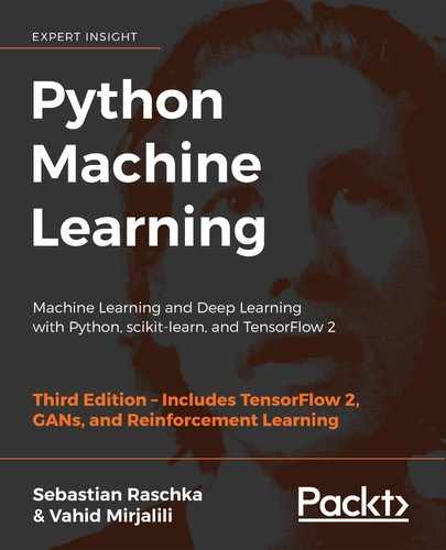
As you can see in the following image, a CNN computes feature maps from an input image, where each element comes from a local patch of pixels in the input image:

This local patch of pixels is referred to as the local receptive field. CNNs will usually perform very well on image-related tasks, and that's largely due to two important ideas:

• Sparse connectivity: A single element in the feature map is connected to only a small patch of pixels. (This is very different from connecting to the whole input image as in the case of perceptrons. You may find it useful to look back and compare how we implemented a fully connected network that connected to the whole image in Chapter 12, Implementing a Multilayer Artificial Neural Network from Scratch.)
• Parameter-sharing: The same weights are used for different patches of the input image.

As a direct consequence of these two ideas, replacing a conventional, fully connected MLP with a convolution layer substantially decreases the number of weights (parameters) in the network and we will see an improvement in the ability to capture salient features. In the context of image data, it makes sense to assume that nearby pixels are typically more relevant to each other than pixels that are far away from each other.

Typically, CNNs are composed of several convolutional and subsampling layers that are followed by one or more fully connected layers at the end. The fully connected layers are essentially an MLP, where every input unit, i, is connected to every output unit, j, with weight (which we covered in more detail in Chapter 12, Implementing a Multilayer Artificial Neural Network from Scratch).

Please note that subsampling layers, commonly known as pooling layers, do not have any learnable parameters; for instance, there are no weights or bias units in pooling layers. However, both the convolutional and fully connected layers have weights and biases that are optimized during training.

In the following sections, we will study convolutional and pooling layers in more detail and see how they work. To understand how convolution operations work, let's start with a convolution in one dimension, which is sometimes used for working with certain types of sequence data, such as text. After discussing one-dimensional convolutions, we will work through the typical two-dimensional ones that are commonly applied to two-dimensional images.

Performing discrete convolutions

A discrete convolution (or simply convolution) is a fundamental operation in a CNN. Therefore, it's important to understand how this operation works. In this section, we will cover the mathematical definition and discuss some of the naive algorithms to compute convolutions of one-dimensional tensors (vectors) and two-dimensional tensors (matrices).

Please note that the formulas and descriptions in this section are solely for understanding how convolution operations in CNNs work. Indeed, much more efficient implementations of convolutional operations already exist in packages such as TensorFlow, as you will see later in this chapter.

Discrete convolutions in one dimension

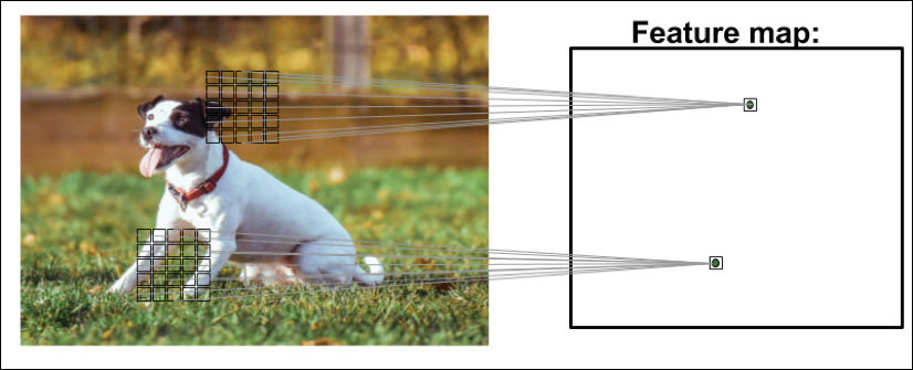
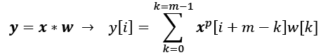
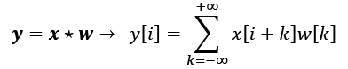
Let's start with some basic definitions and notations that we are going to use. A discrete convolution for two vectors, x and w, is denoted by , in which vector x is our input (sometimes called signal) and w is called the filter or kernel. A discrete convolution is mathematically defined as follows:

As mentioned earlier, the brackets, [ ], are used to denote the indexing for vector elements. The index, i, runs through each element of the output vector, y. There are two odd things in the preceding formula that we need to clarify: to indices and negative indexing for x.

The fact that the sum runs through indices from to seems odd, mainly because in machine learning applications, we always deal with finite feature vectors. For example, if x has 10 features with indices 0, 1, 2,…, 8, 9, then indices and are out of bounds for x. Therefore, to correctly compute the summation shown in the preceding formula, it is assumed that x and w are filled with zeros. This will result in an output vector, y, that also has infinite size, with lots of zeros as well. Since this is not useful in practical situations, x is padded only with a finite number of zeros.

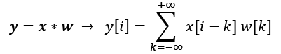
This process is called zero-padding or simply padding. Here, the number of zeros padded on each side is denoted by p. An example padding of a one-dimensional vector, x, is shown in the following figure:

Let's assume that the original input, x, and filter, w, have n and m elements, respectively, where . Therefore, the padded vector, , has size n + 2p. The practical formula for computing a discrete convolution will change to the following:

Now that we have solved the infinite index issue, the second issue is indexing x with i + m – k. The important point to notice here is that x and w are indexed in different directions in this summation. Computing the sum with one index going in the reverse direction is equivalent to computing the sum with both indices in the forward direction after flipping one of those vectors, x or w, after they are padded. Then, we can simply compute their dot product. Let's assume we flip (rotate) the filter, w, to get the rotated filter, . Then, the dot product, , is computed to get one element, y[i], where x[i: i + m] is a patch of x with size m. This operation is repeated like in a sliding window approach to get all the output elements. The following figure provides an example with x = [3 2 1 7 1 2 5 4] and so that the first three output elements are computed:

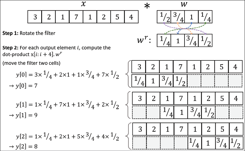
You can see in the preceding example that the padding size is zero (p = 0). Notice that the rotated filter, , is shifted by two cells each time we shift. This shift is another hyperparameter of a convolution, the stride, s. In this example, the stride is two, s = 2. Note that the stride has to be a positive number smaller than the size of the input vector. We will talk more about padding and strides in the next section.

Cross-correlation

Cross-correlation (or simply correlation) between an input vector and a filter is denoted by and is very much like a sibling of a convolution, with a small difference: in cross-correlation, the multiplication is performed in the same direction. Therefore, it is not a requirement to rotate the filter matrix, w, in each dimension. Mathematically, cross-correlation is defined as follows:

The same rules for padding and stride may be applied to cross-correlation as well. Note that most deep learning frameworks (including TensorFlow) implement cross-correlation but refer to it as convolution, which is a common convention in the deep learning field.

Padding inputs to control the size of the output feature maps

So far, we've only used zero-padding in convolutions to compute finite-sized output vectors. Technically, padding can be applied with any . Depending on the choice of p, boundary cells may be treated differently than the cells located in the middle of x.

Now, consider an example where n = 5 and m = 3. Then, with p=0, x[0] is only used in computing one output element (for instance, y[0]), while x[1] is used in the computation of two output elements (for instance, y[0] and y[1]). So, you can see that this different treatment of elements of x can artificially put more emphasis on the middle element, x[2], since it has appeared in most computations. We can avoid this issue if we choose p = 2, in which case, each element of x will be involved in computing three elements of y.

Furthermore, the size of the output, y, also depends on the choice of the padding strategy we use.

There are three modes of padding that are commonly used in practice: full, same, and valid:

• In full mode, the padding parameter, p, is set to p = m – 1. Full padding increases the dimensions of the output; thus, it is rarely used in CNN architectures.
• Same padding is usually used to ensure that the output vector has the same size as the input vector, x. In this case, the padding parameter, p, is computed according to the filter size, along with the requirement that the input size and output size are the same.
• Finally, computing a convolution in the valid mode refers to the case where p = 0 (no padding).

The following figure illustrates the three different padding modes for a simple pixel input with a kernel size of and a stride of 1:

The most commonly used padding mode in CNNs is same padding. One of its advantages over the other padding modes is that same padding preserves the size of the vector—or the height and width of the input images when we are working on image-related tasks in computer vision—which makes designing a network architecture more convenient.

One big disadvantage of valid padding versus full and same padding, for example, is that the volume of the tensors will decrease substantially in NNs with many layers, which can be detrimental to the network performance.

In practice, it is recommended that you preserve the spatial size using same padding for the convolutional layers and decrease the spatial size via pooling layers instead. As for full padding, its size results in an output larger than the input size. Full padding is usually used in signal processing applications where it is important to minimize boundary effects. However, in the deep learning context, boundary effects are usually not an issue, so we rarely see full padding being used in practice.

Determining the size of the convolution output

The output size of a convolution is determined by the total number of times that we shift the filter, w, along the input vector. Let's assume that the input vector is of size n and the filter is of size m. Then, the size of the output resulting from , with padding, p, and stride, s, would be determined as follows:

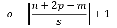
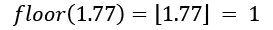
Here, denotes the floor operation.

The floor operation

The floor operation returns the largest integer that is equal to or smaller than the input, for example:

Consider the following two cases:

• Compute the output size for an input vector of size 10 with a convolution kernel of size 5, padding 2, and stride 1:

  

  (Note that in this case, the output size turns out to be the same as the input; therefore, we can conclude this to be the same-padding mode.)

• How does the output size change for the same input vector when we have a kernel of size 3 and stride 2?

  

If you are interested in learning more about the size of the convolution output, we recommend the manuscript A guide to convolution arithmetic for deep learning, by Vincent Dumoulin and Francesco Visin, which is freely available at https://arxiv.org/abs/1603.07285.

Finally, in order to learn how to compute convolutions in one dimension, a naive implementation is shown in the following code block, and the results are compared with the numpy.convolve function. The code is as follows:

>>> import numpy as np
>>> def conv1d(x, w, p=0, s=1):
...     w_rot = np.array(w[::-1])
...     x_padded = np.array(x)
...     if p > 0:
...         zero_pad = np.zeros(shape=p)
...         x_padded = np.concatenate([zero_pad,
...                                    x_padded,
...                                    zero_pad])
...     res = []
...     for i in range(0, int(len(x)/s),s):
...         res.append(np.sum(x_padded[i:i+w_rot.shape[0]] *
...                           w_rot))
...     return np.array(res)
>>> ## Testing:
>>> x = [1, 3, 2, 4, 5, 6, 1, 3]
>>> w = [1, 0, 3, 1, 2]
>>> print('Conv1d Implementation:',
...       conv1d(x, w, p=2, s=1))
Conv1d Implementation: [ 5. 14. 16. 26. 24. 34. 19. 22.]
>>> print('NumPy Results:',
...       np.convolve(x, w, mode='same'))
NumPy Results: [ 5 14 16 26 24 34 19 22]

So far, we have mostly focused on convolutions for vectors (1D convolutions). We started with the 1D case to make the concepts easier to understand. In the next section, we will cover 2D convolutions in more detail, which are the building blocks of CNNs for image-related tasks.

Performing a discrete convolution in 2D

The concepts you learned in the previous sections are easily extendible to 2D. When we deal with 2D inputs, such as a matrix, , and the filter matrix, , where and , then the matrix is the result of a 2D convolution between X and W. This is defined mathematically as follows:

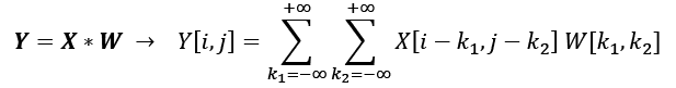
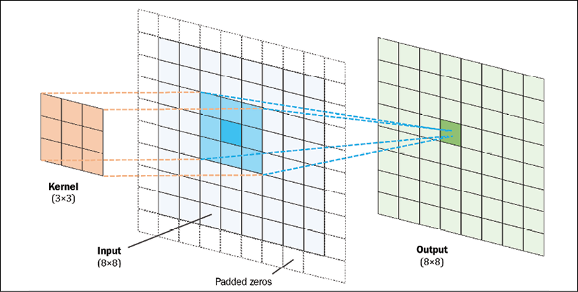
Notice that if you omit one of the dimensions, the remaining formula is exactly the same as the one we used previously to compute the convolution in 1D. In fact, all the previously mentioned techniques, such as zero-padding, rotating the filter matrix, and the use of strides, are also applicable to 2D convolutions, provided that they are extended to both dimensions independently. The following figure demonstrates 2D convolution of an input matrix of size , using a kernel of size . The input matrix is padded with zeros with p = 1. As a result, the output of the 2D convolution will have a size of :

The following example illustrates the computation of a 2D convolution between an input matrix, , and a kernel matrix, , using padding p = (1, 1) and stride s = (2, 2). According to the specified padding, one layer of zeros is added on each side of the input matrix, which results in the padded matrix , as follows:

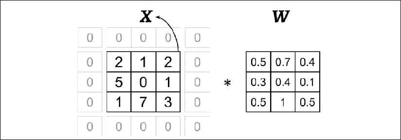
With the preceding filter, the rotated filter will be:

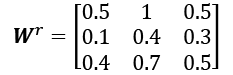
Note that this rotation is not the same as the transpose matrix. To get the rotated filter in NumPy, we can write W_rot=W[::-1,::-1]. Next, we can shift the rotated filter matrix along the padded input matrix, , like a sliding window and compute the sum of the element-wise product, which is denoted by the operator in the following figure:

The result will be the matrix, Y.

Let's also implement the 2D convolution according to the naive algorithm described. The scipy.signal package provides a way to compute 2D convolution via the scipy.signal.convolve2d function:

>>> import numpy as np
>>> import scipy.signal
>>> def conv2d(X, W, p=(0, 0), s=(1, 1)):
...     W_rot = np.array(W)[::-1,::-1]
...     X_orig = np.array(X)
...     n1 = X_orig.shape[0] + 2*p[0]
...     n2 = X_orig.shape[1] + 2*p[1]
...     X_padded = np.zeros(shape=(n1, n2))
...     X_padded[p[0]:p[0]+X_orig.shape[0],
...              p[1]:p[1]+X_orig.shape[1]] = X_orig
...
...     res = []
...     for i in range(0, int((X_padded.shape[0] - 
...                            W_rot.shape[0])/s[0])+1, s[0]):
...         res.append([])
...         for j in range(0, int((X_padded.shape[1] - 
...                                W_rot.shape[1])/s[1])+1, s[1]):
...             X_sub = X_padded[i:i+W_rot.shape[0],
...                              j:j+W_rot.shape[1]]
...             res[-1].append(np.sum(X_sub * W_rot))
...     return(np.array(res))
>>> X = [[1, 3, 2, 4], [5, 6, 1, 3], [1, 2, 0, 2], [3, 4, 3, 2]]
>>> W = [[1, 0, 3], [1, 2, 1], [0, 1, 1]]
>>> print('Conv2d Implementation:
',
...       conv2d(X, W, p=(1, 1), s=(1, 1)))
Conv2d Implementation:
[[ 11.  25.  32.  13.]
 [ 19.  25.  24.  13.]
 [ 13.  28.  25.  17.]
 [ 11.  17.  14.   9.]]
>>> print('SciPy Results:
',
...       scipy.signal.convolve2d(X, W, mode='same'))
SciPy Results:
[[11 25 32 13]
 [19 25 24 13]
 [13 28 25 17]
 [11 17 14  9]]

In the next section, we will discuss subsampling or pooling, which is another important operation often used in CNNs.

Subsampling layers

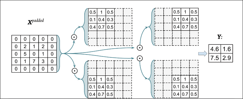
Subsampling is typically applied in two forms of pooling operations in CNNs: max-pooling and mean-pooling (also known as average-pooling). The pooling layer is usually denoted by . Here, the subscript determines the size of the neighborhood (the number of adjacent pixels in each dimension) where the max or mean operation is performed. We refer to such a neighborhood as the pooling size.

The operation is described in the following figure. Here, max-pooling takes the maximum value from a neighborhood of pixels, and mean-pooling computes their average:

The advantage of pooling is twofold:

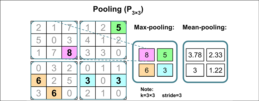
• Pooling (max-pooling) introduces a local invariance. This means that small changes in a local neighborhood do not change the result of max-pooling.

  Therefore, it helps with generating features that are more robust to noise in the input data. Refer to the following example, which shows that the max-pooling of two different input matrices, and , results in the same output:

  

• Pooling decreases the size of features, which results in higher computational efficiency. Furthermore, reducing the number of features may reduce the degree of overfitting as well.

While pooling is still an essential part of many CNN architectures, several CNN architectures have also been developed without using pooling layers. Instead of using pooling layers to reduce the feature size, researchers use convolutional layers with a stride of 2.

In a sense, you can think of a convolutional layer with stride 2 as a pooling layer with learnable weights. If you are interested in an empirical comparison of different CNN architectures developed with and without pooling layers, we recommend reading the research article Striving for Simplicity: The All Convolutional Net, by Jost Tobias Springenberg, Alexey Dosovitskiy, Thomas Brox, and Martin Riedmiller. This article is freely available at https://arxiv.org/abs/1412.6806.

Putting everything together – implementing a CNN

So far, you have learned about the basic building blocks of CNNs. The concepts illustrated in this chapter are not really more difficult than traditional multilayer NNs. We can say that the most important operation in a traditional NN is matrix multiplication. For instance, we use matrix multiplications to compute the pre-activations (or net inputs), as in z = Wx + b. Here, x is a column vector ( matrix) representing pixels, and W is the weight matrix connecting the pixel inputs to each hidden unit.

In a CNN, this operation is replaced by a convolution operation, as in , where X is a matrix representing the pixels in a arrangement. In both cases, the pre-activations are passed to an activation function to obtain the activation of a hidden unit, , where is the activation function. Furthermore, you will recall that subsampling is another building block of a CNN, which may appear in the form of pooling, as was described in the previous section.

Working with multiple input or color channels

An input to a convolutional layer may contain one or more 2D arrays or matrices with dimensions (for example, the image height and width in pixels). These matrices are called channels. Conventional implementations of convolutional layers expect a rank-3 tensor representation as an input, for example a three-dimensional array, , where is the number of input channels. For example, let's consider images as input to the first layer of a CNN. If the image is colored and uses the RGB color mode, then (for the red, green, and blue color channels in RGB). However, if the image is in grayscale, then we have , because there is only one channel with the grayscale pixel intensity values.

>>> import tensorflow as tf
>>> img_raw = tf.io.read_file('example-image.png')
>>> img = tf.image.decode_image(img_raw)
>>> print('Image shape:', img.shape)
Image shape: (252, 221, 3)

> conda install imageio

> pip install imageio

>>> import imageio
>>> img = imageio.imread('example-image.png')
>>> print('Image shape:', img.shape)
Image shape: (252, 221, 3)
>>> print('Number of channels:', img.shape[2])
Number of channels: 3
>>> print('Image data type:', img.dtype)
Image data type: uint8
>>> print(img[100:102, 100:102, :])
[[[179 134 110]
 [182 136 112]]
[[180 135 11]
 [182 137 113]]]

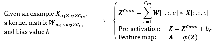
Now that you are familiar with the structure of input data, the next question is, how can we incorporate multiple input channels in the convolution operation that we discussed in the previous sections? The answer is very simple: we perform the convolution operation for each channel separately and then add the results together using the matrix summation. The convolution associated with each channel (c) has its own kernel matrix as W[:, :, c]. The total pre-activation result is computed in the following formula:

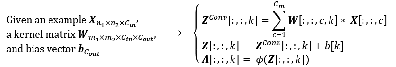
The final result, A, is a feature map. Usually, a convolutional layer of a CNN has more than one feature map. If we use multiple feature maps, the kernel tensor becomes four-dimensional: . Here, is the kernel size, is the number of input channels, and is the number of output feature maps. So, now let's include the number of output feature maps in the preceding formula and update it, as follows:

To conclude our discussion of computing convolutions in the context of NNs, let's look at the example in the following figure, which shows a convolutional layer, followed by a pooling layer. In this example, there are three input channels. The kernel tensor is four-dimensional. Each kernel matrix is denoted as , and there are three of them, one for each input channel. Furthermore, there are five such kernels, accounting for five output feature maps. Finally, there is a pooling layer for subsampling the feature maps:

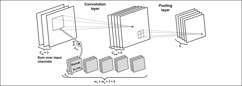
How many trainable parameters exist in the preceding example?

To illustrate the advantages of convolution, parameter-sharing, and sparse connectivity, let's work through an example. The convolutional layer in the network shown in the preceding figure is a four-dimensional tensor. So, there are parameters associated with the kernel. Furthermore, there is a bias vector for each output feature map of the convolutional layer. Thus, the size of the bias vector is 5. Pooling layers do not have any (trainable) parameters; therefore, we can write the following:

If the input tensor is of size , assuming that the convolution is performed with the same-padding mode, then the output feature maps would be of size .

Note that if we use a fully connected layer instead of a convolutional layer, this number will be much larger. In the case of a fully connected layer, the number of parameters for the weight matrix to reach the same number of output units would have been as follows:

In addition, the size of the bias vector is (one bias element for each output unit). Given that and , we can see that the difference in the number of trainable parameters is significant.

Lastly, as was already mentioned, typically, the convolution operations are carried out by treating an input image with multiple color channels as a stack of matrices; that is, we perform the convolution on each matrix separately and then add the results, as was illustrated in the previous figure. However, convolutions can also be extended to 3D volumes if you are working with 3D datasets, for example, as shown in the paper VoxNet: A 3D Convolutional Neural Network for Real-Time Object Recognition (2015), by Daniel Maturana and Sebastian Scherer, which can be accessed at https://www.ri.cmu.edu/pub_files/2015/9/voxnet_maturana_scherer_iros15.pdf.

In the next section, we will talk about how to regularize an NN.

Regularizing an NN with dropout

Choosing the size of a network, whether we are dealing with a traditional (fully connected) NN or a CNN, has always been a challenging problem. For instance, the size of a weight matrix and the number of layers need to be tuned to achieve a reasonably good performance.

You will recall from Chapter 14, Going Deeper – The Mechanics of TensorFlow, that a simple network without any hidden layer could only capture a linear decision boundary, which is not sufficient for dealing with an exclusive or (XOR) or similar problem. The capacity of a network refers to the level of complexity of the function that it can learn to approximate. Small networks, or networks with a relatively small number of parameters, have a low capacity and are therefore likely to underfit, resulting in poor performance, since they cannot learn the underlying structure of complex datasets. However, very large networks may result in overfitting, where the network will memorize the training data and do extremely well on the training dataset while achieving a poor performance on the held-out test dataset. When we deal with real-world machine learning problems, we do not know how large the network should be a priori.

One way to address this problem is to build a network with a relatively large capacity (in practice, we want to choose a capacity that is slightly larger than necessary) to do well on the training dataset. Then, to prevent overfitting, we can apply one or multiple regularization schemes to achieve a good generalization performance on new data, such as the held-out test dataset.

In Chapter 3, A Tour of Machine Learning Classifiers Using scikit-learn, we covered L1 and L2 regularization. In the section Tackling overfitting via regularization, you saw that both techniques, L1 and L2 regularization, can prevent or reduce the effect of overfitting by adding a penalty to the loss that results in shrinking the weight parameters during training. While both L1 and L2 regularization can be used for NNs as well, with L2 being the more common choice of the two, there are other methods for regularizing NNs, such as dropout, which we discuss in this section. But before we move on to discussing dropout, to use L2 regularization within a convolutional or fully connected (dense) network, you can simply add the L2 penalty to the loss function by setting the kernel_regularizer of a particular layer when using the Keras API, as follows (it will then automatically modify the loss function accordingly):

>>> from tensorflow import keras 
>>> conv_layer = keras.layers.Conv2D(
...     filters=16,
...     kernel_size=(3,3),
...     kernel_regularizer=keras.regularizers.l2(0.001))
>>> fc_layer = keras.layers.Dense(
...     units=16,
...     kernel_regularizer=keras.regularizers.l2(0.001))

In recent years, dropout has emerged as a popular technique for regularizing (deep) NNs to avoid overfitting, thus improving the generalization performance (Dropout: a simple way to prevent neural networks from overfitting, by N. Srivastava, G. Hinton, A. Krizhevsky, I. Sutskever, and R. Salakhutdinov, Journal of Machine Learning Research 15.1, pages 1929-1958, 2014, http://www.jmlr.org/papers/volume15/srivastava14a/srivastava14a.pdf). Dropout is usually applied to the hidden units of higher layers and works as follows: during the training phase of an NN, a fraction of the hidden units is randomly dropped at every iteration with probability (or keep probability ). This dropout probability is determined by the user and the common choice is p = 0.5, as discussed in the previously mentioned article by Nitish Srivastava and others, 2014. When dropping a certain fraction of input neurons, the weights associated with the remaining neurons are rescaled to account for the missing (dropped) neurons.

The effect of this random dropout is that the network is forced to learn a redundant representation of the data. Therefore, the network cannot rely on an activation of any set of hidden units, since they may be turned off at any time during training, and is forced to learn more general and robust patterns from the data.

This random dropout can effectively prevent overfitting. The following figure shows an example of applying dropout with probability p = 0.5 during the training phase, whereby half of the neurons will become inactive randomly (dropped units are selected randomly in each forward pass of training). However, during prediction, all neurons will contribute to computing the pre-activations of the next layer.

As shown here, one important point to remember is that units may drop randomly during training only, whereas for the evaluation (inference) phase, all the hidden units must be active (for instance, or ). To ensure that the overall activations are on the same scale during training and prediction, the activations of the active neurons have to be scaled appropriately (for example, by halving the activation if the dropout probability was set to p = 0.5).

However, since it is inconvenient to always scale activations when making predictions, TensorFlow and other tools scale the activations during training (for example, by doubling the activations if the dropout probability was set to p = 0.5). This approach is commonly referred to as inverse dropout.

While the relationship is not immediately obvious, dropout can be interpreted as the consensus (averaging) of an ensemble of models. As discussed in Chapter 7, Combining Different Models for Ensemble Learning, in ensemble learning, we train several models independently. During prediction, we then use the consensus of all the trained models. We already know that model ensembles are known to perform better than single models. In deep learning, however, both training several models and collecting and averaging the output of multiple models is computationally expensive. Here, dropout offers a workaround, with an efficient way to train many models at once and compute their average predictions at test or prediction time.

As mentioned previously, the relationship between model ensembles and dropout is not immediately obvious. However, consider that in dropout, we have a different model for each mini-batch (due to setting the weights to zero randomly during each forward pass).

Then, via iterating over the mini-batches, we essentially sample over models, where h is the number of hidden units.

The restriction and aspect that distinguishes dropout from regular ensembling, however, is that we share the weights over these "different models", which can be seen as a form of regularization. Then, during "inference" (for instance, predicting the labels in the test dataset), we can average over all these different models that we sampled over during training. This is very expensive, though.

Then, averaging the models, that is, computing the geometric mean of the class-membership probability that is returned by a model, i, can be computed as follows:

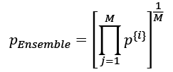
Now, the trick behind dropout is that this geometric mean of the model ensembles (here, M models) can be approximated by scaling the predictions of the last (or final) model sampled during training by a factor of 1/(1 – p), which is much cheaper than computing the geometric mean explicitly using the previous equation. (In fact, the approximation is exactly equivalent to the true geometric mean if we consider linear models.)

Loss functions for classification

In Chapter 13, Parallelizing Neural Network Training with TensorFlow, we saw different activation functions, such as ReLU, sigmoid, and tanh. Some of these activation functions, like ReLU, are mainly used in the intermediate (hidden) layers of an NN to add non-linearities to our model. But others, like sigmoid (for binary) and softmax (for multiclass), are added at the last (output) layer, which results in class-membership probabilities as the output of the model. If the sigmoid or softmax activations are not included at the output layer, then the model will compute the logits instead of the class-membership probabilities.

Focusing on classification problems here, depending on the type of problem (binary versus multiclass) and the type of output (logits versus probabilities), we should choose the appropriate loss function to train our model. Binary cross-entropy is the loss function for a binary classification (with a single output unit), and categorical cross-entropy is the loss function for multiclass classification. In the Keras API, two options for categorical cross-entropy loss are provided, depending on whether the ground truth labels are in a one-hot encoded format (for example, [0, 0, 1, 0]), or provided as integer labels (for example, y=2), which is also known as "sparse" representation in the context of Keras.

The following table describes three loss functions available in Keras for dealing with all three cases: binary classification, multiclass with one-hot encoded ground truth labels, and multiclass with integer (sparse) labels. Each one of these three loss functions also has the option to receive the predictions in the form of logits or class-membership probabilities:

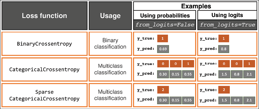
Please note that computing the cross-entropy loss by providing the logits, and not the class-membership probabilities, is usually preferred due to numerical stability reasons. If we provide logits as inputs to the loss function and set from_logits=True, the respective TensorFlow function uses a more efficient implementation to compute the loss and derivative of the loss with respect to the weights. This is possible since certain mathematical terms cancel and thus don't have to be computed explicitly when providing logits as inputs.

The following code will show you how to use these three loss functions with two different formats, where either the logits or class-membership probabilities are given as inputs to the loss functions:

>>> import tensorflow_datasets as tfds
>>> ####### Binary Crossentropy
>>> bce_probas = tf.keras.losses.BinaryCrossentropy(from_logits=False)
>>> bce_logits = tf.keras.losses.BinaryCrossentropy(from_logits=True)
>>> logits = tf.constant([0.8])
>>> probas = tf.keras.activations.sigmoid(logits)
>>> tf.print(
...     'BCE (w Probas): {:.4f}'.format(
...     bce_probas(y_true=[1], y_pred=probas)),
...     '(w Logits): {:.4f}'.format(
...     bce_logits(y_true=[1], y_pred=logits)))
BCE (w Probas): 0.3711 (w Logits): 0.3711
>>> ####### Categorical Crossentropy
>>> cce_probas = tf.keras.losses.CategoricalCrossentropy(
...     from_logits=False)
>>> cce_logits = tf.keras.losses.CategoricalCrossentropy(
...     from_logits=True)
>>> logits = tf.constant([[1.5, 0.8, 2.1]])
>>> probas = tf.keras.activations.softmax(logits)
>>> tf.print(
...     'CCE (w Probas): {:.4f}'.format(
...     cce_probas(y_true=[0, 0, 1], y_pred=probas)),
...     '(w Logits): {:.4f}'.format(
...     cce_logits(y_true=[0, 0, 1], y_pred=logits)))
CCE (w Probas): 0.5996 (w Logits): 0.5996
>>> ####### Sparse Categorical Crossentropy
>>> sp_cce_probas = tf.keras.losses.SparseCategoricalCrossentropy(
...     from_logits=False)
>>> sp_cce_logits = tf.keras.losses.SparseCategoricalCrossentropy(
...     from_logits=True)
>>> tf.print(
...     'Sparse CCE (w Probas): {:.4f}'.format(
...     sp_cce_probas(y_true=[2], y_pred=probas)),
...     '(w Logits): {:.4f}'.format(
...     sp_cce_logits(y_true=[2], y_pred=logits)))
Sparse CCE (w Probas): 0.5996 (w Logits): 0.5996

Note that sometimes, you may come across an implementation where a categorical cross-entropy loss is used for binary classification. Typically, when we have a binary classification task, the model returns a single output value for each example. We interpret this single model output as the probability of the positive class (for example, class 1), P[class = 1]. In a binary classification problem, it is implied that P[class = 0] = 1 – P[class = 1]; hence, we do not need a second output unit in order to obtain the probability of the negative class. However, sometimes practitioners choose to return two outputs for each training example and interpret them as probabilities of each class: P[class = 0] versus P[class = 1]. Then, in such a case, using a softmax function (instead of the logistic sigmoid) to normalize the outputs (so that they sum to 1) is recommended, and categorical cross-entropy is the appropriate loss function.

Implementing a deep CNN using TensorFlow

In Chapter 14, Going Deeper – The Mechanics of TensorFlow, you may recall that we used TensorFlow Estimators for handwritten digit recognition problems, using different API levels of TensorFlow. You may also recall that we achieved about 89 percent accuracy using the DNNClassifier Estimator with two hidden layers.

Now, let's implement a CNN and see whether it can achieve a better predictive performance compared to the MLP (DNNClassifier) for classifying handwritten digits. Note that the fully connected layers that we saw in Chapter 14, Going Deeper – The Mechanics of TensorFlow, were able to perform well on this problem. However, in some applications, such as reading bank account numbers from handwritten digits, even tiny mistakes can be very costly. Therefore, it is crucial to reduce this error as much as possible.

The multilayer CNN architecture

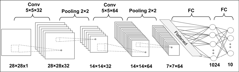
The architecture of the network that we are going to implement is shown in the following figure. The inputs are grayscale images. Considering the number of channels (which is 1 for grayscale images) and a batch of input images, the input tensor's dimensions will be .

The input data goes through two convolutional layers that have a kernel size of . The first convolution has 32 output feature maps, and the second one has 64 output feature maps. Each convolution layer is followed by a subsampling layer in the form of a max-pooling operation, . Then a fully connected layer passes the output to a second fully connected layer, which acts as the final softmax output layer. The architecture of the network that we are going to implement is shown in the following figure:

The dimensions of the tensors in each layer are as follows:

• Input:
• Conv_1:
• Pooling_1:
• Conv_2:
• Pooling_2:
• FC_1:
• FC_2 and softmax layer:

For the convolutional kernels, we are using strides=1 such that the input dimensions are preserved in the resulting feature maps. For the pooling layers, we are using strides=2 to subsample the image and shrink the size of the output feature maps. We will implement this network using the TensorFlow Keras API.

Loading and preprocessing the data

You will recall that in Chapter 13, Parallelizing Neural Network Training with TensorFlow, you learned two ways of loading available datasets from the tensorflow_datasets module. One approach is based on a three-step process, and a simpler method uses a function called load, which wraps those three steps. Here, we will use the first method. The three steps for loading the MNIST dataset are as follows:

>>> import tensorflow_datasets as tfds
>>> ## Loading the data
>>> mnist_bldr = tfds.builder('mnist')
>>> mnist_bldr.download_and_prepare()
>>> datasets = mnist_bldr.as_dataset(shuffle_files=False)
>>> mnist_train_orig = datasets['train']
>>> mnist_test_orig = datasets['test'] 

The MNIST dataset comes with a pre-specified training and test dataset partitioning scheme, but we also want to create a validation split from the train partition. Notice that in the third step, we used an optional argument, shuffle_files=False, in the .as_dataset() method. This prevented initial shuffling, which is necessary for us since we want to split the training dataset into two parts: a smaller training dataset and a validation dataset. (Note: if the initial shuffling was not turned off, it would incur reshuffling of the dataset every time we fetched a mini-batch of data.

An example of this behavior is shown in the online contents of this chapter, where you can see that the number of labels in the validation datasets changes due to reshuffling of the train/validation splits. This can cause false performance estimation of the model, since the train/validation datasets are indeed mixed.) We can split the train/validation datasets as follows:

>>> BUFFER_SIZE = 10000
>>> BATCH_SIZE = 64
>>> NUM_EPOCHS = 20
>>> mnist_train = mnist_train_orig.map(
...     lambda item: (tf.cast(item['image'], tf.float32)/255.0,
...                   tf.cast(item['label'], tf.int32)))
>>> mnist_test = mnist_test_orig.map(
...     lambda item: (tf.cast(item['image'], tf.float32)/255.0,
...                   tf.cast(item['label'], tf.int32)))
>>> tf.random.set_seed(1)
>>> mnist_train = mnist_train.shuffle(buffer_size=BUFFER_SIZE,
...                   reshuffle_each_iteration=False)
>>> mnist_valid = mnist_train.take(10000).batch(BATCH_SIZE)
>>> mnist_train = mnist_train.skip(10000).batch(BATCH_SIZE)

Now, after preparing the dataset, we are ready to implement the CNN we just described.

Implementing a CNN using the TensorFlow Keras API

For implementing a CNN in TensorFlow, we use the Keras Sequential class to stack different layers, such as convolution, pooling, and dropout, as well as the fully connected (dense) layers. The Keras layers API provides classes for each one: tf.keras.layers.Conv2D for a two-dimensional convolution layer; tf.keras.layers.MaxPool2D and tf.keras.layers.AvgPool2D for subsampling (max-pooling and average-pooling); and tf.keras.layers.Dropout for regularization using dropout. We will go over each of these classes in more detail.

Configuring CNN layers in Keras

Constructing a layer with the Conv2D class requires us to specify the number of output filters (which is equivalent to the number of output feature maps) and kernel sizes.

In addition, there are optional parameters that we can use to configure a convolutional layer. The most commonly used ones are the strides (with a default value of 1 in both x, y dimensions) and padding, which could be same or valid. Additional configuration parameters are listed in the official documentation: https://www.tensorflow.org/versions/r2.0/api_docs/python/tf/keras/layers/Conv2D.

It is worth mentioning that usually, when we read an image, the default dimension for the channels is the last dimension of the tensor array. This is called the "NHWC" format, where N stands for the number of images within the batch, H and W stand for height and width, respectively, and C stands for channels.

Note that the Conv2D class assumes that inputs are in the NHWC format by default. (Other tools, such as PyTorch, use an NCHW format.) However, if you come across some data whose channels are placed at the first dimension (the first dimension after the batch dimension, or second dimension considering the batch dimension), you would need to swap the axes in your data to move the channels to the last dimension. Or, an alternative way to work with an NCHW-formatted input is to set data_format="channels_first". After the layer is constructed, it can be called by providing a four-dimensional tensor, with the first dimension reserved for a batch of examples; depending on the data_format argument, either the second or the fourth dimension corresponds to the channel; and the other two dimensions are the spatial dimensions.

As shown in the architecture of the CNN model that we want to build, each convolution layer is followed by a pooling layer for subsampling (reducing the size of feature maps). The MaxPool2D and AvgPool2D classes construct the max-pooling and average-pooling layers, respectively. The argument pool_size determines the size of the window (or neighborhood) that will be used to compute the max or mean operations. Furthermore, the strides parameter can be used to configure the pooling layer, as we discussed earlier.

Finally, the Dropout class will construct the dropout layer for regularization, with the argument rate used to determine the probability of dropping the input units during the training. When calling this layer, its behavior can be controlled via an argument named training, to specify whether this call will be made during training or during the inference.

Constructing a CNN in Keras

Now that you have learned about these classes, we can construct the CNN model that was shown in the previous figure. In the following code, we will use the Sequential class and add the convolution and pooling layers:

>>> model = tf.keras.Sequential()
>>> model.add(tf.keras.layers.Conv2D(
...     filters=32, kernel_size=(5, 5),
...     strides=(1, 1), padding='same',
...     data_format='channels_last',
...     name='conv_1', activation='relu'))
>>> model.add(tf.keras.layers.MaxPool2D(
...     pool_size=(2, 2), name='pool_1'))
>>> model.add(tf.keras.layers.Conv2D(
...     filters=64, kernel_size=(5, 5),
...     strides=(1, 1), padding='same',
...     name='conv_2', activation='relu'))
>>> model.add(tf.keras.layers.MaxPool2D(
...     pool_size=(2, 2), name='pool_2'))

So far, we have added two convolution layers to the model. For each convolutional layer, we used a kernel of size and 'same' padding. As discussed earlier, using padding='same' preserves the spatial dimensions (vertical and horizontal dimensions) of the feature maps such that the inputs and outputs have the same height and width (and the number of channels may only differ in terms of the number of filters used). The max-pooling layers with pooling size and strides of 2 will reduce the spatial dimensions by half. (Note that if the strides parameter is not specified in MaxPool2D, by default, it is set equal to the pooling size.)

While we can calculate the size of the feature maps at this stage manually, the Keras API provides a convenient method to compute this for us:

>>> model.compute_output_shape(input_shape=(16, 28, 28, 1))
TensorShape([16, 7, 7, 64])

By providing the input shape as a tuple specified in this example, the method compute_output_shape calculated the output to have a shape (16, 7, 7, 64), indicating feature maps with 64 channels and a spatial size of . The first dimension corresponds to the batch dimension, for which we used 16 arbitrarily. We could have used None instead, that is, input_shape=(None, 28, 28, 1).

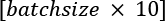
The next layer that we want to add is a dense (or fully connected) layer for implementing a classifier on top of our convolutional and pooling layers. The input to this layer must have rank 2, that is, shape []. Thus, we need to flatten the output of the previous layers to meet this requirement for the dense layer:

>>> model.add(tf.keras.layers.Flatten())
>>> model.compute_output_shape(input_shape=(16, 28, 28, 1))
TensorShape([16, 3136])

As the result of compute_output_shape indicates, the input dimensions for the dense layer are correctly set up. Next, we will add two dense layers with a dropout layer in between:

>>> model.add(tf.keras.layers.Dense(
...     units=1024, name='fc_1',
...     activation='relu'))
>>> model.add(tf.keras.layers.Dropout(
...     rate=0.5))
>>> model.add(tf.keras.layers.Dense(
...     units=10, name='fc_2',
...     activation='softmax'))

The last fully connected layer, named 'fc_2', has 10 output units for the 10 class labels in the MNIST dataset. Also, we use the softmax activation to obtain the class-membership probabilities of each input example, assuming that the classes are mutually exclusive, so the probabilities for each example sum to 1. (This means that a training example can belong to only one class.) Based on what we discussed in the section Loss functions for classification, which loss should we use here? Remember that for a multiclass classification with integer (sparse) labels (as opposed to one-hot encoded labels), we use SparseCategoricalCrossentropy. The following code will call the build() method for late variable creation and compile the model:

>>> tf.random.set_seed(1)
>>> model.build(input_shape=(None, 28, 28, 1))
>>> model.compile(
...     optimizer=tf.keras.optimizers.Adam(),
...     loss=tf.keras.losses.SparseCategoricalCrossentropy(),
...     metrics=['accuracy'])

As you already know, we can train the model by calling the fit() method. Note that using the designated methods for training and evaluation (like evaluate() and predict()) will automatically set the mode for the dropout layer and rescale the hidden units appropriately so that we do not have to worry about that at all. Next, we will train this CNN model and use the validation dataset that we created for monitoring the learning progress:

>>> history = model.fit(mnist_train, epochs=NUM_EPOCHS,
...                     validation_data=mnist_valid,
...                     shuffle=True)
Epoch 1/20
782/782 [==============================] - 35s 45ms/step - loss: 0.1450 - accuracy: 0.8882 - val_loss: 0.0000e+00 - val_accuracy: 0.0000e+00
Epoch 2/20
782/782 [==============================] - 34s 43ms/step - loss: 0.0472 - accuracy: 0.9833 - val_loss: 0.0507 - val_accuracy: 0.9839
..
Epoch 20/20
782/782 [==============================] - 34s 44ms/step - loss: 0.0047 - accuracy: 0.9985 - val_loss: 0.0488 - val_accuracy: 0.9920

Once the 20 epochs of training are finished, we can visualize the learning curves:

>>> import matplotlib.pyplot as plt
>>> hist = history.history
>>> x_arr = np.arange(len(hist['loss'])) + 1
>>> fig = plt.figure(figsize=(12, 4))
>>> ax = fig.add_subplot(1, 2, 1)
>>> ax.plot(x_arr, hist['loss'], '-o', label='Train loss')
>>> ax.plot(x_arr, hist['val_loss'], '--<', label='Validation loss')
>>> ax.legend(fontsize=15)
>>> ax = fig.add_subplot(1, 2, 2)
>>> ax.plot(x_arr, hist['accuracy'], '-o', label='Train acc.')
>>> ax.plot(x_arr, hist['val_accuracy'], '--<', 
...         label='Validation acc.')
>>> ax.legend(fontsize=15)
>>> plt.show()

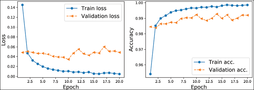
As you already know from the two previous chapters, evaluating the trained model on the test dataset can be done by calling the .evaluate() method:

>>> test_results = model.evaluate(mnist_test.batch(20))
>>> print('Test Acc.: {:.2f}\%'.format(test_results[1]*100))
Test Acc.: 99.39%

The CNN model achieves an accuracy of 99.39%. Remember that in Chapter 14, Going Deeper – The Mechanics of TensorFlow, we got approximately 90% accuracy using the Estimator DNNClassifier.

Finally, we can get the prediction results in the form of class-membership probabilities and convert them to predicted labels by using the tf.argmax function to find the element with the maximum probability. We will do this for a batch of 12 examples and visualize the input and predicted labels:

>>> batch_test = next(iter(mnist_test.batch(12)))
>>> preds = model(batch_test[0])
>>> tf.print(preds.shape)
TensorShape([12, 10])
>>> preds = tf.argmax(preds, axis=1)
>>> print(preds)
tf.Tensor([6 2 3 7 2 2 3 4 7 6 6 9], shape=(12,), dtype=int64)
>>> fig = plt.figure(figsize=(12, 4))
>>> for i in range(12):
...     ax = fig.add_subplot(2, 6, i+1)
...     ax.set_xticks([]); ax.set_yticks([])
...     img = batch_test[0][i, :, :, 0]
...     ax.imshow(img, cmap='gray_r')
...     ax.text(0.9, 0.1, '{}'.format(preds[i]),
...             size=15, color='blue',
...             horizontalalignment='center',
...             verticalalignment='center',
...             transform=ax.transAxes)
>>> plt.show()

The following figure shows the handwritten inputs and their predicted labels:

In this set of plotted examples, all the predicted labels are correct.

We leave the task of showing some of the misclassified digits, as we did in Chapter 12, Implementing a Multilayer Artificial Neural Network from Scratch, as an exercise for the reader.

Gender classification from face images using a CNN

In this section, we are going to implement a CNN for gender classification from face images using the CelebA dataset. As you already saw in Chapter 13, Parallelizing Neural Network Training with TensorFlow, the CelebA dataset contains 202,599 face images of celebrities. In addition, 40 binary facial attributes are available for each image, including gender (male or female) and age (young or old).

Based on what you have learned so far, the goal of this section is to build and train a CNN model for predicting the gender attribute from these face images. Here, for simplicity, we will only be using a small portion of the training data (16,000 training examples) to speed up the training process. However, in order to improve the generalization performance and reduce overfitting on such a small dataset, we will use a technique called data augmentation.

Loading the CelebA dataset

First, let's load the data similarly to how we did in the previous section for the MNIST dataset. CelebA data comes in three partitions: a training dataset, a validation dataset, and a test dataset. Next, we will implement a simple function to count the number of examples in each partition:

>>> import tensorflow as tf
>>> import tensorflow_datasets as tfds
>>> celeba_bldr = tfds.builder('celeb_a')
>>> celeba_bldr.download_and_prepare()
>>> celeba = celeba_bldr.as_dataset(shuffle_files=False)
>>> celeba_train = celeba['train']
>>> celeba_valid = celeba['validation']
>>> celeba_test = celeba['test']
>>>
>>> def count_items(ds):
...     n = 0
...     for _ in ds:
...         n += 1
...     return n
>>> print('Train set:  {}'.format(count_items(celeba_train)))
Train set:  162770
>>> print('Validation: {}'.format(count_items(celeba_valid)))
Validation: 19867
>>> print('Test set:   {}'.format(count_items(celeba_test)))
Test set:   19962

So, instead of using all the available training and validation data, we will take a subset of 16,000 training examples and 1,000 examples for validation, as follows:

>>> celeba_train = celeba_train.take(16000)
>>> celeba_valid = celeba_valid.take(1000)
>>> print('Train set:  {}'.format(count_items(celeba_train)))
Train set:  16000
>>> print('Validation: {}'.format(count_items(celeba_valid)))
Validation: 1000

It is important to note that if the shuffle_files argument in celeba_bldr.as_dataset() was not set to False, we would still see 16,000 examples in the training dataset and 1,000 examples for the validation dataset. However, at each iteration, it would reshuffle the training data and take a new set of 16,000 examples. This would defeat the purpose, as our goal here is to intentionally train our model with a small dataset. Next, we will discuss data augmentation as a technique for boosting the performance of deep NNs.

Image transformation and data augmentation

Data augmentation summarizes a broad set of techniques for dealing with cases where the training data is limited. For instance, certain data augmentation techniques allow us to modify or even artificially synthesize more data and thereby boost the performance of a machine or deep learning model by reducing overfitting. While data augmentation is not only for image data, there are a set of transformations uniquely applicable to image data, such as cropping parts of an image, flipping, changing the contrast, brightness, and saturation. Let's see some of these transformations that are available via the tf.image module. In the following code block, we will first get five examples from the celeba_train dataset and apply five different types of transformation: 1) cropping an image to a bounding box, 2) flipping an image horizontally, 3) adjusting the contrast, 4) adjusting the brightness, and 5) center-cropping an image and resizing the resulting image back to its original size, (218, 178). In the following code, we will visualize the results of these transformations, showing each one in a separate column for comparison:

>>> import matplotlib.pyplot as plt
>>> # take 5 examples
>>> examples = []
>>> for example in celeba_train.take(5):
...     examples.append(example['image'])
>>> fig = plt.figure(figsize=(16, 8.5))
>>> ## Column 1: cropping to a bounding-box
>>> ax = fig.add_subplot(2, 5, 1)
>>> ax.set_title('Crop to a 
bounding-box', size=15)
>>> ax.imshow(examples[0])
>>> ax = fig.add_subplot(2, 5, 6)
>>> img_cropped = tf.image.crop_to_bounding_box(
...     examples[0], 50, 20, 128, 128)
>>> ax.imshow(img_cropped)
>>> ## Column 2: flipping (horizontally)
>>> ax = fig.add_subplot(2, 5, 2)
>>> ax.set_title('Flip (horizontal)', size=15)
>>> ax.imshow(examples[1])
>>> ax = fig.add_subplot(2, 5, 7)
>>> img_flipped = tf.image.flip_left_right(examples[1])
>>> ax.imshow(img_flipped)
>>> ## Column 3: adjust contrast
>>> ax = fig.add_subplot(2, 5, 3)
>>> ax.set_title('Adjust constrast', size=15)
>>> ax.imshow(examples[2])
>>> ax = fig.add_subplot(2, 5, 8)
>>> img_adj_contrast = tf.image.adjust_contrast(
...     examples[2], contrast_factor=2)
>>> ax.imshow(img_adj_contrast)
>>> ## Column 4: adjust brightness
>>> ax = fig.add_subplot(2, 5, 4)
>>> ax.set_title('Adjust brightness', size=15)
>>> ax.imshow(examples[3])
>>> ax = fig.add_subplot(2, 5, 9)
>>> img_adj_brightness = tf.image.adjust_brightness(
...     examples[3], delta=0.3)
>>> ax.imshow(img_adj_brightness)
>>> ## Column 5: cropping from image center
>>> ax = fig.add_subplot(2, 5, 5)
>>> ax.set_title('Centeral crop
and resize', size=15)
>>> ax.imshow(examples[4])
>>> ax = fig.add_subplot(2, 5, 10)
>>> img_center_crop = tf.image.central_crop(
...     examples[4], 0.7)
>>> img_resized = tf.image.resize(
...     img_center_crop, size=(218, 178))
>>> ax.imshow(img_resized.numpy().astype('uint8'))
>>> plt.show()

The following figure shows the results:

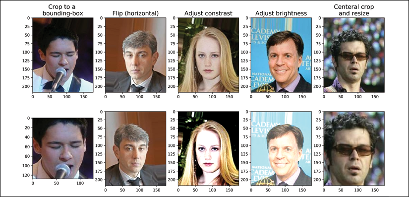
In the previous figure, the original images are shown in the first row and their transformed version in the second row. Note that for the first transformation (leftmost column), the bounding box is specified by four numbers: the coordinate of the upper-left corner of the bounding box (here x=20, y=50), and the width and height of the box (width=128, height=128). Also note that the origin (the coordinates at the location denoted as (0, 0)) for images loaded by TensorFlow (as well as other packages such as imageio) is the upper-left corner of the image.

The transformations in the previous code block are deterministic. However, all such transformations can also be randomized, which is recommended for data augmentation during model training. For example, a random bounding box (where the coordinates of the upper-left corner are selected randomly) can be cropped from an image, an image can be randomly flipped along either the horizontal or vertical axes with a probability of 0.5, or the contrast of an image can be changed randomly, where the contrast_factor is selected at random, but with uniform distribution, from a range of values. In addition, we can create a pipeline of these transformations.

For example, we can first randomly crop an image, then flip it randomly, and finally, resize it to the desired size. The code is as follows (since we have random elements, we set the random seed for reproducibility):

>>> tf.random.set_seed(1)
>>> fig = plt.figure(figsize=(14, 12))
>>> for i,example in enumerate(celeba_train.take(3)):
...     image = example['image']
...
...     ax = fig.add_subplot(3, 4, i*4+1)
...     ax.imshow(image)
...     if i == 0:
...         ax.set_title('Orig', size=15)
...
...     ax = fig.add_subplot(3, 4, i*4+2)
...     img_crop = tf.image.random_crop(image, size=(178, 178, 3))
...     ax.imshow(img_crop)
...     if i == 0:
...         ax.set_title('Step 1: Random crop', size=15)
...
...     ax = fig.add_subplot(3, 4, i*4+3)
...     img_flip = tf.image.random_flip_left_right(img_crop)
...     ax.imshow(tf.cast(img_flip, tf.uint8))
...     if i == 0:
...         ax.set_title('Step 2: Random flip', size=15)
...
...     ax = fig.add_subplot(3, 4, i*4+4)
...     img_resize = tf.image.resize(img_flip, size=(128, 128))
...     ax.imshow(tf.cast(img_resize, tf.uint8))
...     if i == 0:
...         ax.set_title('Step 3: Resize', size=15)
>>> plt.show()

The following figure shows random transformations on three example images:

Note that each time we iterate through these three examples, we get slightly different images due to random transformations.

For convenience, we can define a wrapper function to use this pipeline for data augmentation during model training. In the following code, we will define the function preprocess(), which will receive a dictionary containing the keys 'image' and 'attributes'. The function will return a tuple containing the transformed image and the label extracted from the dictionary of attributes.

We will only apply data augmentation to the training examples, however, and not to the validation or test images. The code is as follows:

>>> def preprocess(example, size=(64, 64), mode='train'):
...     image = example['image']
...     label = example['attributes']['Male']
...     if mode == 'train':
...         image_cropped = tf.image.random_crop(
...             image, size=(178, 178, 3))
...         image_resized = tf.image.resize(
...             image_cropped, size=size)
...         image_flip = tf.image.random_flip_left_right(
...             image_resized)
...         return image_flip/255.0, tf.cast(label, tf.int32)
...     else: # use center- instead of 
...           # random-crops for non-training data
...         image_cropped = tf.image.crop_to_bounding_box(
...             image, offset_height=20, offset_width=0,
...             target_height=178, target_width=178)
...         image_resized = tf.image.resize(
...             image_cropped, size=size)
...         return image_resized/255.0, tf.cast(label, tf.int32)

Now, to see data augmentation in action, let's create a small subset of the training dataset, apply this function to it, and iterate over the dataset five times:

>>> tf.random.set_seed(1)
>>> ds = celeba_train.shuffle(1000, reshuffle_each_iteration=False)
>>> ds = ds.take(2).repeat(5)
>>> ds = ds.map(lambda x:preprocess(x, size=(178, 178), mode='train'))
>>> fig = plt.figure(figsize=(15, 6))
>>> for j,example in enumerate(ds):
...     ax = fig.add_subplot(2, 5, j//2+(j%2)*5+1)
...     ax.set_xticks([])
...     ax.set_yticks([])
...     ax.imshow(example[0])
>>> plt.show()

This figure shows the five resulting transformations for data augmentation on two example images:

Next, we will apply this preprocessing function to our training and validation datasets. We will use an image size of (64, 64). Furthermore, we will specify mode='train' when working with training data and use mode='eval' for the validation data so that the random elements of the data augmentation pipeline will be applied only to the training data:

>>> import numpy as np
>>> BATCH_SIZE = 32
>>> BUFFER_SIZE = 1000
>>> IMAGE_SIZE = (64, 64)
>>> steps_per_epoch = np.ceil(16000/BATCH_SIZE)
>>> ds_train = celeba_train.map(
...     lambda x: preprocess(x, size=IMAGE_SIZE, mode='train'))
>>> ds_train = ds_train.shuffle(buffer_size=BUFFER_SIZE).repeat()
>>> ds_train = ds_train.batch(BATCH_SIZE)
>>> ds_valid = celeba_valid.map(
...     lambda x: preprocess(x, size=IMAGE_SIZE, mode='eval'))
>>> ds_valid = ds_valid.batch(BATCH_SIZE)

Training a CNN gender classifier

By now, building a model with TensorFlow's Keras API and training it should be straightforward. The design of our CNN is as follows: the CNN model receives input images of size (the images have three color channels, using 'channels_last').

The input data goes through four convolutional layers to make 32, 64, 128, and 256 feature maps using filters with kernel a size of . The first three convolution layers are followed by max-pooling, . Two dropout layers are also included for regularization:

>>> model = tf.keras.Sequential([
...     tf.keras.layers.Conv2D(
...         32, (3, 3), padding='same', activation='relu'),
...     tf.keras.layers.MaxPooling2D((2, 2)),
...     tf.keras.layers.Dropout(rate=0.5),
...     
...     tf.keras.layers.Conv2D(
...         64, (3, 3), padding='same', activation='relu'),
...     tf.keras.layers.MaxPooling2D((2, 2)),
...     tf.keras.layers.Dropout(rate=0.5),
...     
...     tf.keras.layers.Conv2D(
...         128, (3, 3), padding='same', activation='relu'),
...     tf.keras.layers.MaxPooling2D((2, 2)),
...     
...     tf.keras.layers.Conv2D(
...         256, (3, 3), padding='same', activation='relu')
>>>     ])

Let's see the shape of the output feature maps after applying these layers:

>>> model.compute_output_shape(input_shape=(None, 64, 64, 3))
TensorShape([None, 8, 8, 256])

There are 256 feature maps (or channels) of size . Now, we can add a fully connected layer to get to the output layer with a single unit. If we reshape (flatten) the feature maps, the number of input units to this fully connected layer will be . Alternatively, let's consider a new layer, called global average-pooling, which computes the average of each feature map separately, thereby reducing the hidden units to 256. We can then add a fully connected layer. Although we have not discussed global average-pooling explicitly, it is conceptually very similar to other pooling layers. Global average-pooling can be viewed, in fact, as a special case of average-pooling when the pooling size is equal to the size of the input feature maps.

To understand this, consider the following figure showing an example of input feature maps of shape . The channels are numbered . The global average-pooling operation calculates the average of each channel so that the output will have shape . (Note: GlobalAveragePooling2D in the Keras API will automatically squeeze the output.

Without squeezing the output, the shape would be , as the global average-pooling would reduce the spatial dimension of to a ):

Therefore, given that, in our case, the shape of the feature maps prior to this layer is , we expect to get 256 units as output, that is, the shape of the output will be . Let's add this layer and recompute the output shape to verify that this is true:

>>> model.add(tf.keras.layers.GlobalAveragePooling2D())
>>> model.compute_output_shape(input_shape=(None, 64, 64, 3))
TensorShape([None, 256])

Finally, we can add a fully connected (dense) layer to get a single output unit. In this case, we can specify the activation function to be 'sigmoid' or just use activation=None, so that the model will output the logits (instead of class-membership probabilities), which is preferred for model training in TensorFlow and Keras due to numerical stability, as discussed earlier:

>>> model.add(tf.keras.layers.Dense(1, activation=None))
>>> tf.random.set_seed(1)
>>> model.build(input_shape=(None, 64, 64, 3))
>>> model.summary()
Model: "sequential"
_________________________________________________________________
Layer (type)                 Output Shape              Param #   
=================================================================
conv2d (Conv2D)              multiple                  896       
_________________________________________________________________
max_pooling2d (MaxPooling2D) multiple                  0         
_________________________________________________________________
dropout (Dropout)            multiple                  0         
_________________________________________________________________
conv2d_1 (Conv2D)            multiple                  18496     
_________________________________________________________________
max_pooling2d_1 (MaxPooling2 multiple                  0         
_________________________________________________________________
dropout_1 (Dropout)          multiple                  0         
_________________________________________________________________
conv2d_2 (Conv2D)            multiple                  73856     
_________________________________________________________________
max_pooling2d_2 (MaxPooling2 multiple                  0         
_________________________________________________________________
conv2d_3 (Conv2D)            multiple                  295168    
_________________________________________________________________
global_average_pooling2d (Gl multiple                  0         
_________________________________________________________________
dense (Dense)                multiple                  257       
=================================================================
Total params: 388,673
Trainable params: 388,673
Non-trainable params: 0
_________________________________________________________________

The next step is to compile the model and, at this time, we have to decide what loss function to use. We have a binary classification with a single output unit, so that means we should use BinaryCrossentropy. In addition, since our last layer does not apply sigmoid activation (we used activation=None), the outputs of our model are logits, not probabilities. Therefore, we will also specify from_logits=True in BinaryCrossentropy so that the loss function applies the sigmoid function internally, which is, due to the underlying code, more efficient than doing it manually. The code for compiling and training the model is as follows:

>>> model.compile(optimizer=tf.keras.optimizers.Adam(),
...     loss=tf.keras.losses.BinaryCrossentropy(from_logits=True),
...               metrics=['accuracy'])
>>> history = model.fit(ds_train, validation_data=ds_valid,
...                     epochs=20,
...                     steps_per_epoch=steps_per_epoch)

Let's now visualize the learning curve and compare the training and validation loss and accuracies after each epoch:

>>> hist = history.history
>>> x_arr = np.arange(len(hist['loss'])) + 1
>>> fig = plt.figure(figsize=(12, 4))
>>> ax = fig.add_subplot(1, 2, 1)
>>> ax.plot(x_arr, hist['loss'], '-o', label='Train loss')
>>> ax.plot(x_arr, hist['val_loss'], '--<', label='Validation loss')
>>> ax.legend(fontsize=15)
>>> ax.set_xlabel('Epoch', size=15)
>>> ax.set_ylabel('Loss', size=15)
>>> ax = fig.add_subplot(1, 2, 2)
>>> ax.plot(x_arr, hist['accuracy'], '-o', label='Train acc.')
>>> ax.plot(x_arr, hist['val_accuracy'], '--<',
...         label='Validation acc.')
>>> ax.legend(fontsize=15)
>>> ax.set_xlabel('Epoch', size=15)
>>> ax.set_ylabel('Accuracy', size=15)
>>> plt.show()

The following figure shows the training and validation losses and accuracies:

As you can see from the learning curves, the losses for the training and validation have not converged to a plateau region. Based on this result, we could have continued training for a few more epochs. Using the fit() method, we can continue training for an additional 10 epochs as follows:

>>> history = model.fit(ds_train, validation_data=ds_valid,
...                     epochs=30, initial_epoch=20,
...                     steps_per_epoch=steps_per_epoch)

Once we are happy with the learning curves, we can evaluate the model on the hold-out test dataset:

>>> ds_test = celeba_test.map(
...   lambda x:preprocess(x, size=IMAGE_SIZE, mode='eval')).batch(32)
>>> test_results = model.evaluate(ds_test)
>>> print('Test Acc: {:.2f}%'.format(test_results[1]*100))
Test Acc: 94.75%

Finally, we already know how to get the prediction results on some test examples using model.predict(). However, remember that the model outputs the logits, not probabilities. If we are interested in the class-membership probabilities for this binary problem with a single output unit, we can use the tf.sigmoid function to compute the probability of class 1. (In the case of a multiclass problem, we would use tf.math.softmax.) In the following code, we will take a small subset of 10 examples from our pre-processed test dataset (ds_test) and run model.predict() to get the logits. Then, we will compute the probabilities of each example being from class 1 (which corresponds to male based on the labels provided in CelebA) and visualize the examples along with their ground truth label and the predicted probabilities. Notice that we first apply unbatch() to the ds_test dataset before taking 10 examples; otherwise, the take() method would return 10 batches of size 32, instead of 10 individual examples:

>>> ds = ds_test.unbatch().take(10)
>>> pred_logits = model.predict(ds.batch(10))
>>> probas = tf.sigmoid(pred_logits)
>>> probas = probas.numpy().flatten()*100
>>> fig = plt.figure(figsize=(15, 7))
>>> for j,example in enumerate(ds):
...     ax = fig.add_subplot(2, 5, j+1)
...     ax.set_xticks([]); ax.set_yticks([])
...     ax.imshow(example[0])
...     if example[1].numpy() == 1:
...         label='M'
...     else:
...         label = 'F'
...     ax.text(
...         0.5, -0.15, 'GT: {:s}
Pr(Male)={:.0f}%'
...         ''.format(label, probas[j]),
...         size=16,
...         horizontalalignment='center',
...         verticalalignment='center',
...         transform=ax.transAxes)
>>> plt.tight_layout()
>>> plt.show()

In the following figure, you can see 10 example images along with their ground truth labels and the probabilities that they belong to class 1, male:

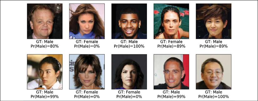
The probabilities of class 1 (that is, male according to CelebA) are provided below each image. As you can see, our trained model made only one error on this set of 10 test examples.

As an optional exercise, you are encouraged to try using the entire training dataset instead of the small subset we created. Furthermore, you can change or modify the CNN architecture. For example, you can change the dropout probabilities and the number of filters in the different convolutional layers. Also, you could replace the global average-pooling with a dense layer. If you are using the entire training dataset with the CNN architecture we trained in this chapter, you should be able to achieve about 97-99% accuracy.

Summary

In this chapter, we learned about CNNs and their main components. We started with the convolution operation and looked at 1D and 2D implementations. Then, we covered another type of layer that is found in several common CNN architectures: the subsampling or so-called pooling layers. We primarily focused on the two most common forms of pooling: max-pooling and average-pooling.

Next, putting all these individual concepts together, we implemented deep CNNs using the TensorFlow Keras API. The first network we implemented was applied to the already familiar MNIST handwritten digit recognition problem.

Then, we implemented a second CNN on a more complex dataset consisting of face images and trained the CNN for gender classification. Along the way, you also learned about data augmentation and different transformations that we can apply to face images using the TensorFlow Dataset class.

In the next chapter, we will move on to recurrent neural networks (RNNs). RNNs are used for learning the structure of sequence data, and they have some fascinating applications, including language translation and image captioning.