The quality of the data and the amount of useful information that it contains are key factors that determine how well a machine learning algorithm can learn. Therefore, it is absolutely critical to ensure that we examine and preprocess a dataset before we feed it to a learning algorithm. In this chapter, we will discuss the essential data preprocessing techniques that will help us to build good machine learning models.

The topics that we will cover in this chapter are as follows:

• Removing and imputing missing values from the dataset
• Getting categorical data into shape for machine learning algorithms
• Selecting relevant features for the model construction

Dealing with missing data

It is not uncommon in real-world applications for our training examples to be missing one or more values for various reasons. There could have been an error in the data collection process, certain measurements may not be applicable, or particular fields could have been simply left blank in a survey, for example. We typically see missing values as blank spaces in our data table or as placeholder strings such as NaN, which stands for "not a number," or NULL (a commonly used indicator of unknown values in relational databases). Unfortunately, most computational tools are unable to handle such missing values or will produce unpredictable results if we simply ignore them. Therefore, it is crucial that we take care of those missing values before we proceed with further analyses.

In this section, we will work through several practical techniques for dealing with missing values by removing entries from our dataset or imputing missing values from other training examples and features.

Identifying missing values in tabular data

Before we discuss several techniques for dealing with missing values, let's create a simple example data frame from a comma-separated values (CSV) file to get a better grasp of the problem:

>>> import pandas as pd
>>> from io import StringIO
>>> csv_data = 
... '''A,B,C,D
... 1.0,2.0,3.0,4.0
... 5.0,6.0,,8.0
... 10.0,11.0,12.0,'''
>>> # If you are using Python 2.7, you need
>>> # to convert the string to unicode:
>>> # csv_data = unicode(csv_data)
>>> df = pd.read_csv(StringIO(csv_data))
>>> df
        A        B        C        D
0     1.0      2.0      3.0      4.0
1     5.0      6.0      NaN      8.0
2    10.0     11.0     12.0      NaN

Using the preceding code, we read CSV-formatted data into a pandas DataFrame via the read_csv function and noticed that the two missing cells were replaced by NaN. The StringIO function in the preceding code example was simply used for the purposes of illustration. It allowed us to read the string assigned to csv_data into a pandas DataFrame as if it was a regular CSV file on our hard drive.

For a larger DataFrame, it can be tedious to look for missing values manually; in this case, we can use the isnull method to return a DataFrame with Boolean values that indicate whether a cell contains a numeric value (False) or if data is missing (True). Using the sum method, we can then return the number of missing values per column as follows:

>>> df.isnull().sum()
A      0
B      0
C      1
D      1
dtype: int64

This way, we can count the number of missing values per column; in the following subsections, we will take a look at different strategies for how to deal with this missing data.

>>> df.values
array([[  1.,   2.,   3.,   4.],
       [  5.,   6.,  nan,   8.],
       [ 10.,  11.,  12.,  nan]])

Eliminating training examples or features with missing values

One of the easiest ways to deal with missing data is simply to remove the corresponding features (columns) or training examples (rows) from the dataset entirely; rows with missing values can easily be dropped via the dropna method:

>>> df.dropna(axis=0)
      A    B    C    D
0   1.0  2.0  3.0  4.0

Similarly, we can drop columns that have at least one NaN in any row by setting the axis argument to 1:

>>> df.dropna(axis=1)
      A      B
0   1.0    2.0
1   5.0    6.0
2  10.0   11.0

The dropna method supports several additional parameters that can come in handy:

# only drop rows where all columns are NaN
# (returns the whole array here since we don't
# have a row with all values NaN)
>>> df.dropna(how='all')
      A      B      C      D
0   1.0    2.0    3.0    4.0
1   5.0    6.0    NaN    8.0
2  10.0   11.0   12.0    NaN
# drop rows that have fewer than 4 real values
>>> df.dropna(thresh=4)
      A      B      C      D
0   1.0    2.0    3.0    4.0
# only drop rows where NaN appear in specific columns (here: 'C')
>>> df.dropna(subset=['C'])
      A      B      C      D
0   1.0    2.0    3.0    4.0
2  10.0   11.0   12.0    NaN

Although the removal of missing data seems to be a convenient approach, it also comes with certain disadvantages; for example, we may end up removing too many samples, which will make a reliable analysis impossible. Or, if we remove too many feature columns, we will run the risk of losing valuable information that our classifier needs to discriminate between classes. In the next section, we will look at one of the most commonly used alternatives for dealing with missing values: interpolation techniques.

Imputing missing values

Often, the removal of training examples or dropping of entire feature columns is simply not feasible, because we might lose too much valuable data. In this case, we can use different interpolation techniques to estimate the missing values from the other training examples in our dataset. One of the most common interpolation techniques is mean imputation, where we simply replace the missing value with the mean value of the entire feature column. A convenient way to achieve this is by using the SimpleImputer class from scikit-learn, as shown in the following code:

>>> from sklearn.impute import SimpleImputer
>>> import numpy as np
>>> imr = SimpleImputer(missing_values=np.nan, strategy='mean')
>>> imr = imr.fit(df.values)
>>> imputed_data = imr.transform(df.values)
>>> imputed_data
array([[  1.,   2.,   3.,   4.],
       [  5.,   6.,  7.5,   8.],
       [ 10.,  11.,  12.,   6.]])

Here, we replaced each NaN value with the corresponding mean, which is separately calculated for each feature column. Other options for the strategy parameter are median or most_frequent, where the latter replaces the missing values with the most frequent values. This is useful for imputing categorical feature values, for example, a feature column that stores an encoding of color names, such as red, green, and blue. We will encounter examples of such data later in this chapter.

Alternatively, an even more convenient way to impute missing values is by using pandas' fillna method and providing an imputation method as an argument. For example, using pandas, we could achieve the same mean imputation directly in the DataFrame object via the following command:

>>> df.fillna(df.mean())

Understanding the scikit-learn estimator API

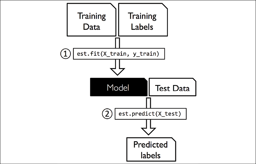
In the previous section, we used the SimpleImputer class from scikit-learn to impute missing values in our dataset. The SimpleImputer class belongs to the so-called transformer classes in scikit-learn, which are used for data transformation. The two essential methods of those estimators are fit and transform. The fit method is used to learn the parameters from the training data, and the transform method uses those parameters to transform the data. Any data array that is to be transformed needs to have the same number of features as the data array that was used to fit the model.

The following figure illustrates how a transformer, fitted on the training data, is used to transform a training dataset as well as a new test dataset:

The classifiers that we used in Chapter 3, A Tour of Machine Learning Classifiers Using scikit-learn, belong to the so-called estimators in scikit-learn, with an API that is conceptually very similar to the transformer class. Estimators have a predict method but can also have a transform method, as you will see later in this chapter. As you may recall, we also used the fit method to learn the parameters of a model when we trained those estimators for classification. However, in supervised learning tasks, we additionally provide the class labels for fitting the model, which can then be used to make predictions about new, unlabeled data examples via the predict method, as illustrated in the following figure:

Handling categorical data

So far, we have only been working with numerical values. However, it is not uncommon for real-world datasets to contain one or more categorical feature columns. In this section, we will make use of simple yet effective examples to see how to deal with this type of data in numerical computing libraries.

When we are talking about categorical data, we have to further distinguish between ordinal and nominal features. Ordinal features can be understood as categorical values that can be sorted or ordered. For example, t-shirt size would be an ordinal feature, because we can define an order: XL > L > M. In contrast, nominal features don't imply any order and, to continue with the previous example, we could think of t-shirt color as a nominal feature since it typically doesn't make sense to say that, for example, red is larger than blue.

Categorical data encoding with pandas

Before we explore different techniques for handling such categorical data, let's create a new DataFrame to illustrate the problem:

>>> import pandas as pd
>>> df = pd.DataFrame([
...            ['green', 'M', 10.1, 'class2'],
...            ['red', 'L', 13.5, 'class1'],
...            ['blue', 'XL', 15.3, 'class2']])
>>> df.columns = ['color', 'size', 'price', 'classlabel']
>>> df
    color  size  price  classlabel
0   green     M   10.1      class2
1     red     L   13.5      class1
2    blue    XL   15.3      class2

As we can see in the preceding output, the newly created DataFrame contains a nominal feature (color), an ordinal feature (size), and a numerical feature (price) column. The class labels (assuming that we created a dataset for a supervised learning task) are stored in the last column. The learning algorithms for classification that we discuss in this book do not use ordinal information in class labels.

Mapping ordinal features

To make sure that the learning algorithm interprets the ordinal features correctly, we need to convert the categorical string values into integers. Unfortunately, there is no convenient function that can automatically derive the correct order of the labels of our size feature, so we have to define the mapping manually. In the following simple example, let's assume that we know the numerical difference between features, for example, XL = L + 1 = M + 2:

>>> size_mapping = {'XL': 3,
...                 'L': 2,
...                 'M': 1}
>>> df['size'] = df['size'].map(size_mapping)
>>> df
    color  size  price  classlabel
0   green     1   10.1      class2
1     red     2   13.5      class1
2    blue     3   15.3      class2

If we want to transform the integer values back to the original string representation at a later stage, we can simply define a reverse-mapping dictionary, inv_size_mapping = {v: k for k, v in size_mapping.items()}, which can then be used via the pandas map method on the transformed feature column and is similar to the size_mapping dictionary that we used previously. We can use it as follows:

>>> inv_size_mapping = {v: k for k, v in size_mapping.items()}
>>> df['size'].map(inv_size_mapping)
0   M
1   L
2   XL
Name: size, dtype: object

Encoding class labels

Many machine learning libraries require that class labels are encoded as integer values. Although most estimators for classification in scikit-learn convert class labels to integers internally, it is considered good practice to provide class labels as integer arrays to avoid technical glitches. To encode the class labels, we can use an approach similar to the mapping of ordinal features discussed previously. We need to remember that class labels are not ordinal, and it doesn't matter which integer number we assign to a particular string label. Thus, we can simply enumerate the class labels, starting at 0:

>>> import numpy as np
>>> class_mapping = {label: idx for idx, label in
...                  enumerate(np.unique(df['classlabel']))}
>>> class_mapping
{'class1': 0, 'class2': 1}

Next, we can use the mapping dictionary to transform the class labels into integers:

>>> df['classlabel'] = df['classlabel'].map(class_mapping)
>>> df
    color  size  price  classlabel
0   green     1   10.1           1
1     red     2   13.5           0
2    blue     3   15.3           1

We can reverse the key-value pairs in the mapping dictionary as follows to map the converted class labels back to the original string representation:

>>> inv_class_mapping = {v: k for k, v in class_mapping.items()}
>>> df['classlabel'] = df['classlabel'].map(inv_class_mapping)
>>> df
    color  size  price  classlabel
0   green     1   10.1      class2
1     red     2   13.5      class1
2    blue     3   15.3      class2

Alternatively, there is a convenient LabelEncoder class directly implemented in scikit-learn to achieve this:

>>> from sklearn.preprocessing import LabelEncoder
>>> class_le = LabelEncoder()
>>> y = class_le.fit_transform(df['classlabel'].values)
>>> y
array([1, 0, 1])

Note that the fit_transform method is just a shortcut for calling fit and transform separately, and we can use the inverse_transform method to transform the integer class labels back into their original string representation:

>>> class_le.inverse_transform(y)
array(['class2', 'class1', 'class2'], dtype=object)

Performing one-hot encoding on nominal features

In the previous Mapping ordinal features section, we used a simple dictionary-mapping approach to convert the ordinal size feature into integers. Since scikit-learn's estimators for classification treat class labels as categorical data that does not imply any order (nominal), we used the convenient LabelEncoder to encode the string labels into integers. It may appear that we could use a similar approach to transform the nominal color column of our dataset, as follows:

>>> X = df[['color', 'size', 'price']].values
>>> color_le = LabelEncoder()
>>> X[:, 0] = color_le.fit_transform(X[:, 0])
>>> X
array([[1, 1, 10.1],
       [2, 2, 13.5],
       [0, 3, 15.3]], dtype=object)

After executing the preceding code, the first column of the NumPy array, X, now holds the new color values, which are encoded as follows:

• blue = 0
• green = 1
• red = 2

If we stop at this point and feed the array to our classifier, we will make one of the most common mistakes in dealing with categorical data. Can you spot the problem? Although the color values don't come in any particular order, a learning algorithm will now assume that green is larger than blue, and red is larger than green. Although this assumption is incorrect, the algorithm could still produce useful results. However, those results would not be optimal.

A common workaround for this problem is to use a technique called one-hot encoding. The idea behind this approach is to create a new dummy feature for each unique value in the nominal feature column. Here, we would convert the color feature into three new features: blue, green, and red. Binary values can then be used to indicate the particular color of an example; for example, a blue example can be encoded as blue=1, green=0, red=0. To perform this transformation, we can use the OneHotEncoder that is implemented in scikit-learn's preprocessing module:

>>> from sklearn.preprocessing import OneHotEncoder
>>> X = df[['color', 'size', 'price']].values
>>> color_ohe = OneHotEncoder()
>>> color_ohe.fit_transform(X[:, 0].reshape(-1, 1)).toarray()
    array([[0., 1., 0.],
           [0., 0., 1.],
           [1., 0., 0.]])

Note that we applied the OneHotEncoder to only a single column, (X[:, 0].reshape(-1, 1))), to avoid modifying the other two columns in the array as well. If we want to selectively transform columns in a multi-feature array, we can use the ColumnTransformer, which accepts a list of (name, transformer, column(s)) tuples as follows:

>>> from sklearn.compose import ColumnTransformer
>>> X = df[['color', 'size', 'price']].values
>>> c_transf = ColumnTransformer([ 
...     ('onehot', OneHotEncoder(), [0]),
...     ('nothing', 'passthrough', [1, 2])
... ])
>>> c_transf.fit_transform(X).astype(float)
    array([[0.0, 1.0, 0.0, 1, 10.1],
           [0.0, 0.0, 1.0, 2, 13.5],
           [1.0, 0.0, 0.0, 3, 15.3]])

In the preceding code example, we specified that we want to modify only the first column and leave the other two columns untouched via the 'passthrough' argument.

An even more convenient way to create those dummy features via one-hot encoding is to use the get_dummies method implemented in pandas. Applied to a DataFrame, the get_dummies method will only convert string columns and leave all other columns unchanged:

>>> pd.get_dummies(df[['price', 'color', 'size']])
    price  size  color_blue  color_green  color_red
0    10.1     1           0            1          0
1    13.5     2           0            0          1
2    15.3     3           1            0          0

When we are using one-hot encoding datasets, we have to keep in mind that this introduces multicollinearity, which can be an issue for certain methods (for instance, methods that require matrix inversion). If features are highly correlated, matrices are computationally difficult to invert, which can lead to numerically unstable estimates. To reduce the correlation among variables, we can simply remove one feature column from the one-hot encoded array. Note that we do not lose any important information by removing a feature column, though; for example, if we remove the column color_blue, the feature information is still preserved since if we observe color_green=0 and color_red=0, it implies that the observation must be blue.

If we use the get_dummies function, we can drop the first column by passing a True argument to the drop_first parameter, as shown in the following code example:

>>> pd.get_dummies(df[['price', 'color', 'size']],
...                drop_first=True)
    price  size  color_green  color_red
0    10.1     1            1          0
1    13.5     2            0          1
2    15.3     3            0          0

In order to drop a redundant column via the OneHotEncoder, we need to set drop='first' and set categories='auto' as follows:

>>> color_ohe = OneHotEncoder(categories='auto', drop='first')
>>> c_transf = ColumnTransformer([
...            ('onehot', color_ohe, [0]),
...            ('nothing', 'passthrough', [1, 2])
... ])
>>> c_transf.fit_transform(X).astype(float)
array([[  1. ,  0. ,  1. ,  10.1],
       [  0. ,  1. ,  2. ,  13.5],
       [  0. ,  0. ,  3. ,  15.3]])

>>> df = pd.DataFrame([['green', 'M', 10.1,
...                     'class2'],
...                    ['red', 'L', 13.5,
...                     'class1'],
...                    ['blue', 'XL', 15.3,
...                     'class2']])
>>> df.columns = ['color', 'size', 'price',
...               'classlabel']
>>> df

>>> df['x > M'] = df['size'].apply(
...     lambda x: 1 if x in {'L', 'XL'} else 0)
>>> df['x > L'] = df['size'].apply(
...     lambda x: 1 if x == 'XL' else 0)
>>> del df['size']
>>> df

Partitioning a dataset into separate training and test datasets

We briefly introduced the concept of partitioning a dataset into separate datasets for training and testing in Chapter 1, Giving Computers the Ability to Learn from Data, and Chapter 3, A Tour of Machine Learning Classifiers Using scikit-learn. Remember that comparing predictions to true labels in the test set can be understood as the unbiased performance evaluation of our model before we let it loose on the real world. In this section, we will prepare a new dataset, the Wine dataset. After we have preprocessed the dataset, we will explore different techniques for feature selection to reduce the dimensionality of a dataset.

The Wine dataset is another open source dataset that is available from the UCI machine learning repository (https://archive.ics.uci.edu/ml/datasets/Wine); it consists of 178 wine examples with 13 features describing their different chemical properties.

df = pd.read_csv(
    'https://archive.ics.uci.edu/ml/'
    'machine-learning-databases/wine/wine.data',
    header=None)

df = pd.read_csv(
    'your/local/path/to/wine.data', header=None)

Using the pandas library, we will directly read in the open source Wine dataset from the UCI machine learning repository:

>>> df_wine = pd.read_csv('https://archive.ics.uci.edu/'
...                       'ml/machine-learning-databases/'
...                       'wine/wine.data', header=None)
>>> df_wine.columns = ['Class label', 'Alcohol',
...                    'Malic acid', 'Ash',
...                    'Alcalinity of ash', 'Magnesium',
...                    'Total phenols', 'Flavanoids',
...                    'Nonflavanoid phenols',
...                    'Proanthocyanins',
...                    'Color intensity', 'Hue',
...                    'OD280/OD315 of diluted wines',
...                    'Proline']
>>> print('Class labels', np.unique(df_wine['Class label']))
Class labels [1 2 3]
>>> df_wine.head()

The 13 different features in the Wine dataset, describing the chemical properties of the 178 wine examples, are listed in the following table:

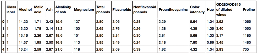
The examples belong to one of three different classes, 1, 2, and 3, which refer to the three different types of grape grown in the same region in Italy but derived from different wine cultivars, as described in the dataset summary (https://archive.ics.uci.edu/ml/machine-learning-databases/wine/wine.names).

A convenient way to randomly partition this dataset into separate test and training datasets is to use the train_test_split function from scikit-learn's model_selection submodule:

>>> from sklearn.model_selection import train_test_split
>>> X, y = df_wine.iloc[:, 1:].values, df_wine.iloc[:, 0].values
>>> X_train, X_test, y_train, y_test =
...     train_test_split(X, y,
...                      test_size=0.3,
...                      random_state=0,
...                      stratify=y)

First, we assigned the NumPy array representation of the feature columns 1-13 to the variable X and we assigned the class labels from the first column to the variable y. Then, we used the train_test_split function to randomly split X and y into separate training and test datasets. By setting test_size=0.3, we assigned 30 percent of the wine examples to X_test and y_test, and the remaining 70 percent of the examples were assigned to X_train and y_train, respectively. Providing the class label array y as an argument to stratify ensures that both training and test datasets have the same class proportions as the original dataset.

Bringing features onto the same scale

Feature scaling is a crucial step in our preprocessing pipeline that can easily be forgotten. Decision trees and random forests are two of the very few machine learning algorithms where we don't need to worry about feature scaling. Those algorithms are scale invariant. However, the majority of machine learning and optimization algorithms behave much better if features are on the same scale, as we saw in Chapter 2, Training Simple Machine Learning Algorithms for Classification, when we implemented the gradient descent optimization algorithm.

The importance of feature scaling can be illustrated by a simple example. Let's assume that we have two features where one feature is measured on a scale from 1 to 10 and the second feature is measured on a scale from 1 to 100,000, respectively.

When we think of the squared error function in Adaline from Chapter 2, Training Simple Machine Learning Algorithms for Classification, it makes sense to say that the algorithm will mostly be busy optimizing the weights according to the larger errors in the second feature. Another example is the k-nearest neighbors (KNN) algorithm with a Euclidean distance measure: the computed distances between examples will be dominated by the second feature axis.

Now, there are two common approaches to bringing different features onto the same scale: normalization and standardization. Those terms are often used quite loosely in different fields, and the meaning has to be derived from the context. Most often, normalization refers to the rescaling of the features to a range of [0, 1], which is a special case of min-max scaling. To normalize our data, we can simply apply the min-max scaling to each feature column, where the new value, , of an example, , can be calculated as follows:

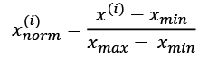
Here, is a particular example, is the smallest value in a feature column, and is the largest value.

The min-max scaling procedure is implemented in scikit-learn and can be used as follows:

>>> from sklearn.preprocessing import MinMaxScaler
>>> mms = MinMaxScaler()
>>> X_train_norm = mms.fit_transform(X_train)
>>> X_test_norm = mms.transform(X_test)

Although normalization via min-max scaling is a commonly used technique that is useful when we need values in a bounded interval, standardization can be more practical for many machine learning algorithms, especially for optimization algorithms such as gradient descent. The reason is that many linear models, such as the logistic regression and SVM from Chapter 3, A Tour of Machine Learning Classifiers Using scikit-learn, initialize the weights to 0 or small random values close to 0. Using standardization, we center the feature columns at mean 0 with standard deviation 1 so that the feature columns have the same parameters as a standard normal distribution (zero mean and unit variance), which makes it easier to learn the weights. Furthermore, standardization maintains useful information about outliers and makes the algorithm less sensitive to them in contrast to min-max scaling, which scales the data to a limited range of values.

The procedure for standardization can be expressed by the following equation:

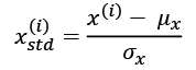
Here, is the sample mean of a particular feature column, and is the corresponding standard deviation.

The following table illustrates the difference between the two commonly used feature scaling techniques, standardization and normalization, on a simple example dataset consisting of numbers 0 to 5:

You can perform the standardization and normalization shown in the table manually by executing the following code examples:

>>> ex = np.array([0, 1, 2, 3, 4, 5])
>>> print('standardized:', (ex - ex.mean()) / ex.std())
standardized: [-1.46385011  -0.87831007  -0.29277002  0.29277002
0.87831007  1.46385011]
>>> print('normalized:', (ex - ex.min()) / (ex.max() - ex.min()))
normalized: [ 0.  0.2  0.4  0.6  0.8  1. ]

Similar to the MinMaxScaler class, scikit-learn also implements a class for standardization:

>>> from sklearn.preprocessing import StandardScaler
>>> stdsc = StandardScaler()
>>> X_train_std = stdsc.fit_transform(X_train)
>>> X_test_std = stdsc.transform(X_test)

Again, it is also important to highlight that we fit the StandardScaler class only once—on the training data—and use those parameters to transform the test dataset or any new data point.

Other, more advanced methods for feature scaling are available from scikit-learn, such as the RobustScaler. The RobustScaler is especially helpful and recommended if we are working with small datasets that contain many outliers. Similarly, if the machine learning algorithm applied to this dataset is prone to overfitting, the RobustScaler can be a good choice. Operating on each feature column independently, the RobustScaler removes the median value and scales the dataset according to the 1st and 3rd quartile of the dataset (that is, the 25th and 75th quantile, respectively) such that more extreme values and outliers become less pronounced. The interested reader can find more information about the RobustScaler in the official scikit-learn documentation at https://scikit-learn.org/stable/modules/generated/sklearn.preprocessing.RobustScaler.html.

Selecting meaningful features

If we notice that a model performs much better on a training dataset than on the test dataset, this observation is a strong indicator of overfitting. As we discussed in Chapter 3, A Tour of Machine Learning Classifiers Using scikit-learn, overfitting means the model fits the parameters too closely with regard to the particular observations in the training dataset, but does not generalize well to new data; we say that the model has a high variance. The reason for the overfitting is that our model is too complex for the given training data. Common solutions to reduce the generalization error are as follows:

• Collect more training data
• Introduce a penalty for complexity via regularization
• Choose a simpler model with fewer parameters
• Reduce the dimensionality of the data

Collecting more training data is often not applicable. In Chapter 6, Learning Best Practices for Model Evaluation and Hyperparameter Tuning, we will learn about a useful technique to check whether more training data is helpful. In the following sections, we will look at common ways to reduce overfitting by regularization and dimensionality reduction via feature selection, which leads to simpler models by requiring fewer parameters to be fitted to the data.

L1 and L2 regularization as penalties against model complexity

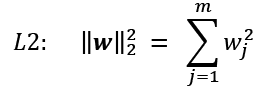
You will recall from Chapter 3, A Tour of Machine Learning Classifiers Using scikit-learn, that L2 regularization is one approach to reduce the complexity of a model by penalizing large individual weights. We defined the squared L2 norm of our weight vector, w, as follows:

Another approach to reduce the model complexity is the related L1 regularization:

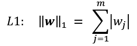
Here, we simply replaced the square of the weights by the sum of the absolute values of the weights. In contrast to L2 regularization, L1 regularization usually yields sparse feature vectors and most feature weights will be zero. Sparsity can be useful in practice if we have a high-dimensional dataset with many features that are irrelevant, especially in cases where we have more irrelevant dimensions than training examples. In this sense, L1 regularization can be understood as a technique for feature selection.

A geometric interpretation of L2 regularization

As mentioned in the previous section, L2 regularization adds a penalty term to the cost function that effectively results in less extreme weight values compared to a model trained with an unregularized cost function.

To better understand how L1 regularization encourages sparsity, let's take a step back and take a look at a geometric interpretation of regularization. Let's plot the contours of a convex cost function for two weight coefficients, and .

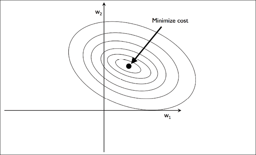
Here, we will consider the sum of squared errors (SSE) cost function that we used for Adaline in Chapter 2, Training Simple Machine Learning Algorithms for Classification, since it is spherical and easier to draw than the cost function of logistic regression; however, the same concepts apply. Remember that our goal is to find the combination of weight coefficients that minimize the cost function for the training data, as shown in the following figure (the point in the center of the ellipses):

We can think of regularization as adding a penalty term to the cost function to encourage smaller weights; in other words, we penalize large weights. Thus, by increasing the regularization strength via the regularization parameter, , we shrink the weights toward zero and decrease the dependence of our model on the training data. Let's illustrate this concept in the following figure for the L2 penalty term:

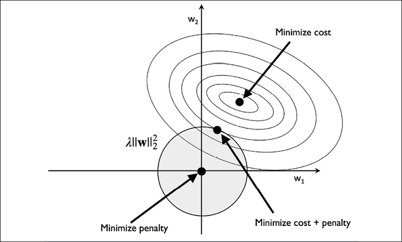
The quadratic L2 regularization term is represented by the shaded ball. Here, our weight coefficients cannot exceed our regularization budget—the combination of the weight coefficients cannot fall outside the shaded area. On the other hand, we still want to minimize the cost function. Under the penalty constraint, our best effort is to choose the point where the L2 ball intersects with the contours of the unpenalized cost function. The larger the value of the regularization parameter, , gets, the faster the penalized cost grows, which leads to a narrower L2 ball. For example, if we increase the regularization parameter towards infinity, the weight coefficients will become effectively zero, denoted by the center of the L2 ball. To summarize the main message of the example, our goal is to minimize the sum of the unpenalized cost plus the penalty term, which can be understood as adding bias and preferring a simpler model to reduce the variance in the absence of sufficient training data to fit the model.

Sparse solutions with L1 regularization

Now, let's discuss L1 regularization and sparsity. The main concept behind L1 regularization is similar to what we discussed in the previous section. However, since the L1 penalty is the sum of the absolute weight coefficients (remember that the L2 term is quadratic), we can represent it as a diamond-shape budget, as shown in the following figure:

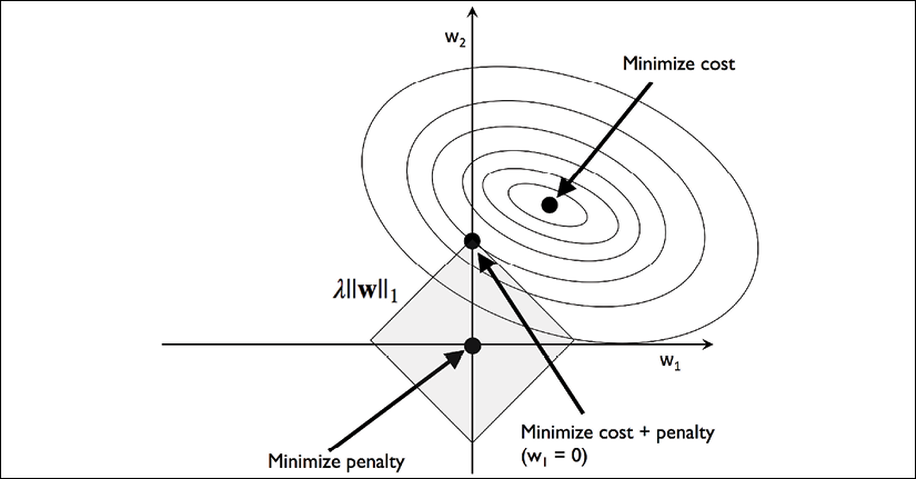
In the preceding figure, we can see that the contour of the cost function touches the L1 diamond at . Since the contours of an L1 regularized system are sharp, it is more likely that the optimum—that is, the intersection between the ellipses of the cost function and the boundary of the L1 diamond—is located on the axes, which encourages sparsity.

For regularized models in scikit-learn that support L1 regularization, we can simply set the penalty parameter to 'l1' to obtain a sparse solution:

>>> from sklearn.linear_model import LogisticRegression
>>> LogisticRegression(penalty='l1',
...                    solver='liblinear',
...                    multi_class='ovr')

Note that we also need to select a different optimization algorithm (for example, solver='liblinear'), since 'lbfgs' currently does not support L1-regularized loss optimization. Applied to the standardized Wine data, the L1 regularized logistic regression would yield the following sparse solution:

>>> lr = LogisticRegression(penalty='l1',
...                         C=1.0,
...                         solver='liblinear',
...                         multi_class='ovr')
# Note that C=1.0 is the default. You can increase
# or decrease it to make the regularization effect
# stronger or weaker, respectively.
>>> lr.fit(X_train_std, y_train)
>>> print('Training accuracy:', lr.score(X_train_std, y_train))
Training accuracy: 1.0
>>> print('Test accuracy:', lr.score(X_test_std, y_test))
Test accuracy: 1.0

Both training and test accuracies (both 100 percent) indicate that our model does a perfect job on both datasets. When we access the intercept terms via the lr.intercept_ attribute, we can see that the array returns three values:

>>> lr.intercept_
array([-1.26346036, -1.21584018, -2.3697841 ])

Since we fit the LogisticRegression object on a multiclass dataset via the one-vs.-rest (OvR) approach, the first intercept belongs to the model that fits class 1 versus classes 2 and 3, the second value is the intercept of the model that fits class 2 versus classes 1 and 3, and the third value is the intercept of the model that fits class 3 versus classes 1 and 2:

>>> lr.coef_
array([[ 1.24590762,  0.18070219,  0.74375939, -1.16141503,
         0.        ,  0.        ,  1.16926815,  0.        ,
         0.        ,  0.        ,  0.        ,  0.54784923,
         2.51028042],
       [-1.53680415, -0.38795309, -0.99494046,  0.36508729,
        -0.05981561,  0.        ,  0.6681573 ,  0.        ,
         0.        , -1.93426485,  1.23265994,  0.        ,
        -2.23137595],
       [ 0.13547047,  0.16873019,  0.35728003,  0.        ,
         0.        ,  0.        , -2.43713947,  0.        ,
         0.        ,  1.56351492, -0.81894749, -0.49308407,
         0.        ]])

The weight array that we accessed via the lr.coef_ attribute contains three rows of weight coefficients, one weight vector for each class. Each row consists of 13 weights, where each weight is multiplied by the respective feature in the 13-dimensional Wine dataset to calculate the net input:

As a result of L1 regularization, which, as mentioned, serves as a method for feature selection, we just trained a model that is robust to the potentially irrelevant features in this dataset. Strictly speaking, though, the weight vectors from the previous example are not necessarily sparse because they contain more non-zero than zero entries. However, we could enforce sparsity (more zero entries) by further increasing the regularization strength—that is, choosing lower values for the C parameter.

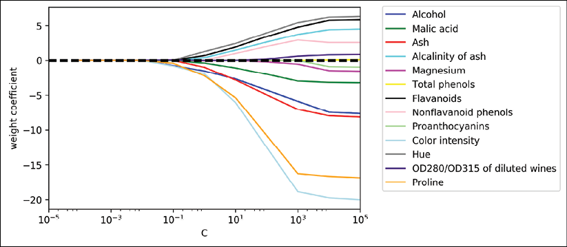
In the last example on regularization in this chapter, we will vary the regularization strength and plot the regularization path—the weight coefficients of the different features for different regularization strengths:

>>> import matplotlib.pyplot as plt
>>> fig = plt.figure()
>>> ax = plt.subplot(111)
>>> colors = ['blue', 'green', 'red', 'cyan',
...           'magenta', 'yellow', 'black',
...           'pink', 'lightgreen', 'lightblue',
...           'gray', 'indigo', 'orange']
>>> weights, params = [], []
>>> for c in np.arange(-4., 6.):
...     lr = LogisticRegression(penalty='l1', C=10.**c,
...                             solver='liblinear',
...                             multi_class='ovr', random_state=0)
...     lr.fit(X_train_std, y_train)
...     weights.append(lr.coef_[1])
...     params.append(10**c)
>>> weights = np.array(weights)
>>> for column, color in zip(range(weights.shape[1]), colors):
...     plt.plot(params, weights[:, column],
...              label=df_wine.columns[column + 1],
...              color=color)
>>> plt.axhline(0, color='black', linestyle='--', linewidth=3)
>>> plt.xlim([10**(-5), 10**5])
>>> plt.ylabel('weight coefficient')
>>> plt.xlabel('C')
>>> plt.xscale('log')
>>> plt.legend(loc='upper left')
>>> ax.legend(loc='upper center',
...           bbox_to_anchor=(1.38, 1.03),
...           ncol=1, fancybox=True)
>>> plt.show()

The resulting plot provides us with further insights into the behavior of L1 regularization. As we can see, all feature weights will be zero if we penalize the model with a strong regularization parameter (C < 0.01); C is the inverse of the regularization parameter, :

Sequential feature selection algorithms

An alternative way to reduce the complexity of the model and avoid overfitting is dimensionality reduction via feature selection, which is especially useful for unregularized models. There are two main categories of dimensionality reduction techniques: feature selection and feature extraction. Via feature selection, we select a subset of the original features, whereas in feature extraction, we derive information from the feature set to construct a new feature subspace.

In this section, we will take a look at a classic family of feature selection algorithms. In the next chapter, Chapter 5, Compressing Data via Dimensionality Reduction, we will learn about different feature extraction techniques to compress a dataset onto a lower-dimensional feature subspace.

Sequential feature selection algorithms are a family of greedy search algorithms that are used to reduce an initial d-dimensional feature space to a k-dimensional feature subspace where k<d. The motivation behind feature selection algorithms is to automatically select a subset of features that are most relevant to the problem, to improve computational efficiency, or to reduce the generalization error of the model by removing irrelevant features or noise, which can be useful for algorithms that don't support regularization.

A classic sequential feature selection algorithm is sequential backward selection (SBS), which aims to reduce the dimensionality of the initial feature subspace with a minimum decay in the performance of the classifier to improve upon computational efficiency. In certain cases, SBS can even improve the predictive power of the model if a model suffers from overfitting.

The idea behind the SBS algorithm is quite simple: SBS sequentially removes features from the full feature subset until the new feature subspace contains the desired number of features. In order to determine which feature is to be removed at each stage, we need to define the criterion function, J, that we want to minimize.

The criterion calculated by the criterion function can simply be the difference in performance of the classifier before and after the removal of a particular feature. Then, the feature to be removed at each stage can simply be defined as the feature that maximizes this criterion; or in more simple terms, at each stage we eliminate the feature that causes the least performance loss after removal. Based on the preceding definition of SBS, we can outline the algorithm in four simple steps:

1. Initialize the algorithm with k = d, where d is the dimensionality of the full feature space, .
2. Determine the feature, , that maximizes the criterion: , where .
3. Remove the feature, , from the feature set: .
4. Terminate if k equals the number of desired features; otherwise, go to step 2.

Unfortunately, the SBS algorithm has not been implemented in scikit-learn yet. But since it is so simple, let's go ahead and implement it in Python from scratch:

from sklearn.base import clone
from itertools import combinations
import numpy as np
from sklearn.metrics import accuracy_score
from sklearn.model_selection import train_test_split
class SBS():
    def __init__(self, estimator, k_features,
                 scoring=accuracy_score,
                 test_size=0.25, random_state=1):
        self.scoring = scoring
        self.estimator = clone(estimator)
        self.k_features = k_features
        self.test_size = test_size
        self.random_state = random_state
    def fit(self, X, y):
        X_train, X_test, y_train, y_test = 
            train_test_split(X, y, test_size=self.test_size,
                             random_state=self.random_state)
    
        dim = X_train.shape[1]
        self.indices_ = tuple(range(dim))
        self.subsets_ = [self.indices_]
        score = self._calc_score(X_train, y_train,
                                 X_test, y_test, self.indices_)
        self.scores_ = [score]
        while dim > self.k_features:
            scores = []
            subsets = []
            
            for p in combinations(self.indices_, r=dim - 1):
                score = self._calc_score(X_train, y_train,
                                         X_test, y_test, p)
                scores.append(score)
                subsets.append(p)
                
            best = np.argmax(scores)
            self.indices_ = subsets[best]
            self.subsets_.append(self.indices_)
            dim -= 1
            
            self.scores_.append(scores[best])
        self.k_score_ = self.scores_[-1]
        
        return self
        
    def transform(self, X):
        return X[:, self.indices_]
    
    def _calc_score(self, X_train, y_train, X_test, y_test, indices):
        self.estimator.fit(X_train[:, indices], y_train)
        y_pred = self.estimator.predict(X_test[:, indices])
        score = self.scoring(y_test, y_pred)
        return score

In the preceding implementation, we defined the k_features parameter to specify the desired number of features we want to return. By default, we use the accuracy_score from scikit-learn to evaluate the performance of a model (an estimator for classification) on the feature subsets.

Inside the while loop of the fit method, the feature subsets created by the itertools.combination function are evaluated and reduced until the feature subset has the desired dimensionality. In each iteration, the accuracy score of the best subset is collected in a list, self.scores_, based on the internally created test dataset, X_test. We will use those scores later to evaluate the results. The column indices of the final feature subset are assigned to self.indices_, which we can use via the transform method to return a new data array with the selected feature columns. Note that, instead of calculating the criterion explicitly inside the fit method, we simply removed the feature that is not contained in the best performing feature subset.

Now, let's see our SBS implementation in action using the KNN classifier from scikit-learn:

>>> import matplotlib.pyplot as plt
>>> from sklearn.neighbors import KNeighborsClassifier
>>> knn = KNeighborsClassifier(n_neighbors=5)
>>> sbs = SBS(knn, k_features=1)
>>> sbs.fit(X_train_std, y_train)

Although our SBS implementation already splits the dataset into a test and training dataset inside the fit function, we still fed the training dataset, X_train, to the algorithm. The SBS fit method will then create new training subsets for testing (validation) and training, which is why this test set is also called the validation dataset. This approach is necessary to prevent our original test set from becoming part of the training data.

Remember that our SBS algorithm collects the scores of the best feature subset at each stage, so let's move on to the more exciting part of our implementation and plot the classification accuracy of the KNN classifier that was calculated on the validation dataset. The code is as follows:

>>> k_feat = [len(k) for k in sbs.subsets_]
>>> plt.plot(k_feat, sbs.scores_, marker='o')
>>> plt.ylim([0.7, 1.02])
>>> plt.ylabel('Accuracy')
>>> plt.xlabel('Number of features')
>>> plt.grid()
>>> plt.tight_layout()
>>> plt.show()

As we can see in the following figure, the accuracy of the KNN classifier improved on the validation dataset as we reduced the number of features, which is likely due to a decrease in the curse of dimensionality that we discussed in the context of the KNN algorithm in Chapter 3, A Tour of Machine Learning Classifiers Using scikit-learn. Also, we can see in the following plot that the classifier achieved 100 percent accuracy for k={3, 7, 8, 9, 10, 11, 12}:

To satisfy our own curiosity, let's see what the smallest feature subset (k=3), which yielded such a good performance on the validation dataset, looks like:

>>> k3 = list(sbs.subsets_[10])
>>> print(df_wine.columns[1:][k3])
Index(['Alcohol', 'Malic acid', 'OD280/OD315 of diluted wines'], dtype='object')

Using the preceding code, we obtained the column indices of the three-feature subset from the 11th position in the sbs.subsets_ attribute and returned the corresponding feature names from the column index of the pandas Wine DataFrame.

Next, let's evaluate the performance of the KNN classifier on the original test dataset:

>>> knn.fit(X_train_std, y_train)
>>> print('Training accuracy:', knn.score(X_train_std, y_train))
Training accuracy: 0.967741935484
>>> print('Test accuracy:', knn.score(X_test_std, y_test))
Test accuracy: 0.962962962963

In the preceding code section, we used the complete feature set and obtained approximately 97 percent accuracy on the training dataset and approximately 96 percent accuracy on the test dataset, which indicates that our model already generalizes well to new data. Now, let's use the selected three-feature subset and see how well KNN performs:

>>> knn.fit(X_train_std[:, k3], y_train)
>>> print('Training accuracy:',
...       knn.score(X_train_std[:, k3], y_train))
Training accuracy: 0.951612903226
>>> print('Test accuracy:',
...       knn.score(X_test_std[:, k3], y_test))
Test accuracy: 0.925925925926

When using less than a quarter of the original features in the Wine dataset, the prediction accuracy on the test dataset declined slightly. This may indicate that those three features do not provide less discriminatory information than the original dataset. However, we also have to keep in mind that the Wine dataset is a small dataset and is very susceptible to randomness—that is, the way we split the dataset into training and test subsets, and how we split the training dataset further into a training and validation subset.

While we did not increase the performance of the KNN model by reducing the number of features, we shrank the size of the dataset, which can be useful in real-world applications that may involve expensive data collection steps. Also, by substantially reducing the number of features, we obtain simpler models, which are easier to interpret.

Assessing feature importance with random forests

In previous sections, you learned how to use L1 regularization to zero out irrelevant features via logistic regression and how to use the SBS algorithm for feature selection and apply it to a KNN algorithm. Another useful approach for selecting relevant features from a dataset is using a random forest, an ensemble technique that was introduced in Chapter 3, A Tour of Machine Learning Classifiers Using scikit-learn. Using a random forest, we can measure the feature importance as the averaged impurity decrease computed from all decision trees in the forest, without making any assumptions about whether our data is linearly separable or not. Conveniently, the random forest implementation in scikit-learn already collects the feature importance values for us so that we can access them via the feature_importances_ attribute after fitting a RandomForestClassifier. By executing the following code, we will now train a forest of 500 trees on the Wine dataset and rank the 13 features by their respective importance measures—remember from our discussion in Chapter 3, A Tour of Machine Learning Classifiers Using scikit-learn that we don't need to use standardized or normalized features in tree-based models:

>>> from sklearn.ensemble import RandomForestClassifier
>>> feat_labels = df_wine.columns[1:]
>>> forest = RandomForestClassifier(n_estimators=500,
...                                 random_state=1)
>>> forest.fit(X_train, y_train)
>>> importances = forest.feature_importances_
>>> indices = np.argsort(importances)[::-1]
>>> for f in range(X_train.shape[1]):
...     print("%2d) %-*s %f" % (f + 1, 30,
...                             feat_labels[indices[f]],
...                             importances[indices[f]]))
>>> plt.title('Feature Importance')
>>> plt.bar(range(X_train.shape[1]),
...         importances[indices],
...         align='center')
>>> plt.xticks(range(X_train.shape[1]),
...            feat_labels[indices] rotation=90)
>>> plt.xlim([-1, X_train.shape[1]])
>>> plt.tight_layout()
>>> plt.show()
 1) Proline                         0.185453
 2) Flavanoids                      0.174751
 3) Color intensity                 0.143920
 4) OD280/OD315 of diluted wines    0.136162
 5) Alcohol                         0.118529
 6) Hue                             0.058739
 7) Total phenols                   0.050872
 8) Magnesium                       0.031357
 9) Malic acid                      0.025648
 10) Proanthocyanins                0.025570
 11) Alcalinity of ash              0.022366
 12) Nonflavanoid phenols           0.013354
 13) Ash                            0.013279

After executing the code, we created a plot that ranks the different features in the Wine dataset by their relative importance; note that the feature importance values are normalized so that they sum up to 1.0:

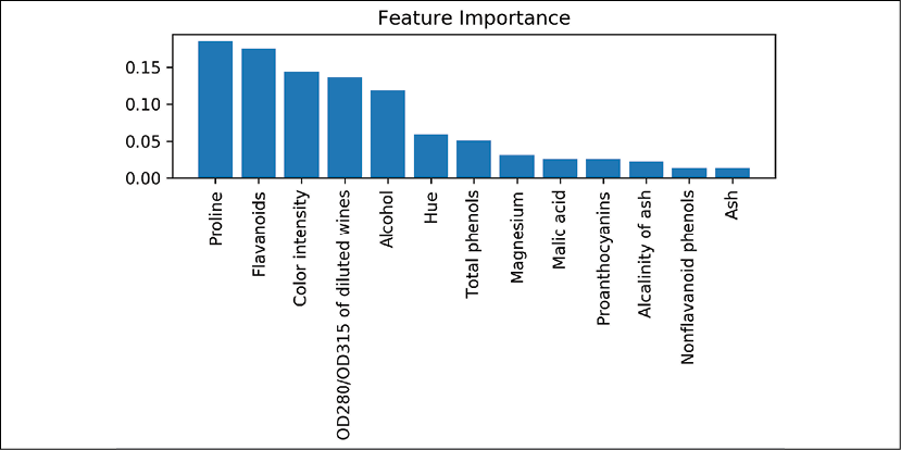
We can conclude that the proline and flavonoid levels, the color intensity, the OD280/OD315 diffraction, and the alcohol concentration of wine are the most discriminative features in the dataset based on the average impurity decrease in the 500 decision trees. Interestingly, two of the top-ranked features in the plot are also in the three-feature subset selection from the SBS algorithm that we implemented in the previous section (alcohol concentration and OD280/OD315 of diluted wines).

However, as far as interpretability is concerned, the random forest technique comes with an important gotcha that is worth mentioning. If two or more features are highly correlated, one feature may be ranked very highly while the information on the other feature(s) may not be fully captured. On the other hand, we don't need to be concerned about this problem if we are merely interested in the predictive performance of a model rather than the interpretation of feature importance values.

To conclude this section about feature importance values and random forests, it is worth mentioning that scikit-learn also implements a SelectFromModel object that selects features based on a user-specified threshold after model fitting, which is useful if we want to use the RandomForestClassifier as a feature selector and intermediate step in a scikit-learn Pipeline object, which allows us to connect different preprocessing steps with an estimator, as you will see in Chapter 6, Learning Best Practices for Model Evaluation and Hyperparameter Tuning. For example, we could set the threshold to 0.1 to reduce the dataset to the five most important features using the following code:

>>> from sklearn.feature_selection import SelectFromModel
>>> sfm = SelectFromModel(forest, threshold=0.1, prefit=True)
>>> X_selected = sfm.transform(X_train)
>>> print('Number of features that meet this threshold', 
...       'criterion:', X_selected.shape[1])
Number of features that meet this threshold criterion: 5
>>> for f in range(X_selected.shape[1]):
...     print("%2d) %-*s %f" % (f + 1, 30,
...                             feat_labels[indices[f]],
...                             importances[indices[f]]))
 1) Proline                         0.185453
 2) Flavanoids                      0.174751
 3) Color intensity                 0.143920
 4) OD280/OD315 of diluted wines    0.136162
 5) Alcohol                         0.118529

Summary

We started this chapter by looking at useful techniques to make sure that we handle missing data correctly. Before we feed data to a machine learning algorithm, we also have to make sure that we encode categorical variables correctly, and in this chapter, we saw how we can map ordinal and nominal feature values to integer representations.

Moreover, we briefly discussed L1 regularization, which can help us to avoid overfitting by reducing the complexity of a model. As an alternative approach to removing irrelevant features, we used a sequential feature selection algorithm to select meaningful features from a dataset.

In the next chapter, you will learn about yet another useful approach to dimensionality reduction: feature extraction. It allows us to compress features onto a lower-dimensional subspace, rather than removing features entirely as in feature selection.