In Chapter 13, Parallelizing Neural Network Training with TensorFlow, we covered how to define and manipulate tensors and worked with the tf.data API to build input pipelines. We further built and trained a multilayer perceptron to classify the Iris dataset using the TensorFlow Keras API (tf.keras).
Now that we have some hands-on experience with TensorFlow neural network (NN) training and machine learning, it's time to take a deeper dive into the TensorFlow library and explore its rich set of features, which will allow us to implement more advanced deep learning models in upcoming chapters.
In this chapter, we will use different aspects of TensorFlow's API to implement NNs. In particular, we will again use the Keras API, which provides multiple layers of abstraction to make the implementation of standard architectures very convenient. TensorFlow also allows us to implement custom NN layers, which is very useful in research-oriented projects that require more customization. Later in this chapter, we will implement such a custom layer.
To illustrate the different ways of model building using the Keras API, we will also consider the classic exclusive or (XOR) problem. Firstly, we will build multilayer perceptrons using the Sequential class. Then, we will consider other methods, such as subclassing tf.keras.Model for defining custom layers. Finally, we will cover tf.estimator, a high-level TensorFlow API that encapsulates the machine learning steps from raw input to prediction.
The topics that we will cover are as follows:
- Understanding and working with TensorFlow graphs and migration to TensorFlow v2
- Function decoration for graph compilation
- Working with TensorFlow variables
- Solving the classic XOR problem and understanding model capacity
- Building complex NN models using Keras'
Modelclass and the Keras functional API - Computing gradients using automatic differentiation and
tf.GradientTape - Working with TensorFlow Estimators
The key features of TensorFlow
TensorFlow provides us with a scalable, multiplatform programming interface for implementing and running machine learning algorithms. The TensorFlow API has been relatively stable and mature since its 1.0 release in 2017, but it just experienced a major redesign with its recent 2.0 release in 2019, which we are using in this book.
Since its initial release in 2015, TensorFlow has become the most widely adopted deep learning library. However, one of its main friction points was that it was built around static computation graphs. Static computation graphs have certain advantages, such as better graph optimizations behind the scenes and support for a wider range of hardware devices; however, static computation graphs require separate graph declaration and graph evaluation steps, which make it cumbersome for users to develop and work with NNs interactively.
Taking all the user feedback to heart, the TensorFlow team decided to make dynamic computation graphs the default in TensorFlow 2.0, which makes the development and training of NNs much more convenient. In the next section, we will cover some of the important changes from TensorFlow v1.x to v2. Dynamic computation graphs allow for interleaving the graph declaration and graph evaluation steps such that TensorFlow 2.0 feels much more natural for Python and NumPy users compared to previous versions of TensorFlow. However, note that TensorFlow 2.0 still allows users to use the "old" TensorFlow v1.x API via the tf.compat submodule. This helps users to transition their code bases more smoothly to the new TensorFlow v2 API.
A key feature of TensorFlow, which was also noted in Chapter 13, Parallelizing Neural Network Training with TensorFlow, is its ability to work with single or multiple graphical processing units (GPUs). This allows users to train deep learning models very efficiently on large datasets and large-scale systems.
While TensorFlow is an open source library and can be freely used by everyone, its development is funded and supported by Google. This involves a large team of software engineers who expand and improve the library continuously. Since TensorFlow is an open source library, it also has strong support from other developers outside of Google, who avidly contribute and provide user feedback.
This has made the TensorFlow library more useful to both academic researchers and developers. A further consequence of these factors is that TensorFlow has extensive documentation and tutorials to help new users.
Last, but not least, TensorFlow supports mobile deployment, which also makes it a very suitable tool for production.
TensorFlow's computation graphs: migrating to TensorFlow v2
TensorFlow performs its computations based on a directed acyclic graph (DAG). In TensorFlow v1.x, such graphs could be explicitly defined in the low-level API, although this was not trivial for large and complex models. In this section, we will see how these graphs can be defined for a simple arithmetic computation. Then, we will see how to migrate a graph to TensorFlow v2, the eager execution and dynamic graph paradigm, as well as the function decoration for faster computations.
Understanding computation graphs
TensorFlow relies on building a computation graph at its core, and it uses this computation graph to derive relationships between tensors from the input all the way to the output. Let's say that we have rank 0 (scalar) tensors a, b, and c and we want to evaluate ![]() . This evaluation can be represented as a computation graph, as shown in the following figure:
. This evaluation can be represented as a computation graph, as shown in the following figure:
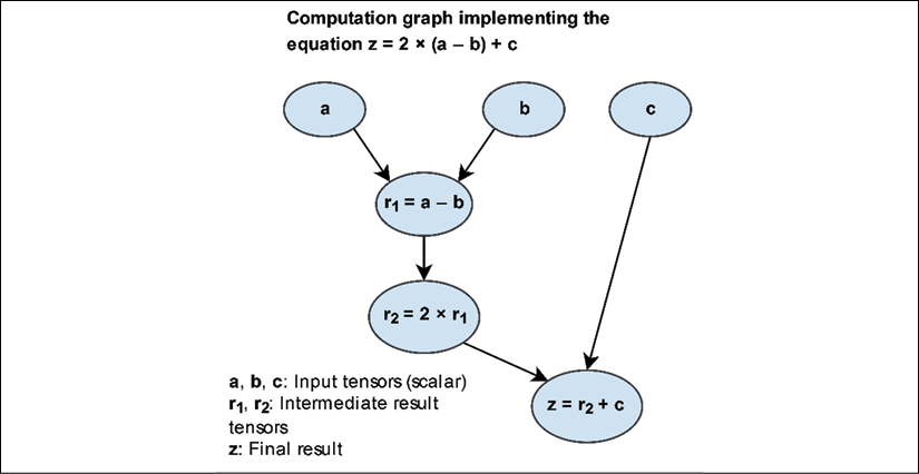
As you can see, the computation graph is simply a network of nodes. Each node resembles an operation, which applies a function to its input tensor or tensors and returns zero or more tensors as the output. TensorFlow builds this computation graph and uses it to compute the gradients accordingly. In the next subsections, we will see some examples of creating a graph for this computation using TensorFlow v1.x and v2 styles.
Creating a graph in TensorFlow v1.x
In the earlier version of the TensorFlow (v1.x) low-level API, this graph had to be explicitly declared. The individual steps for building, compiling, and evaluating such a computation graph in TensorFlow v1.x are as follows:
- Instantiate a new, empty computation graph
- Add nodes (tensors and operations) to the computation graph
- Evaluate (execute) the graph:
- Start a new session
- Initialize the variables in the graph
- Run the computation graph in this session
Before we take a look at the dynamic approach in TensorFlow v2, let's look at a simple example that illustrates how to create a graph in TensorFlow v1.x for evaluating ![]() , as shown in the previous figure. The variables a, b, and c are scalars (single numbers), and we define these as TensorFlow constants. A graph can then be created by calling
, as shown in the previous figure. The variables a, b, and c are scalars (single numbers), and we define these as TensorFlow constants. A graph can then be created by calling tf.Graph(). Variables, as well as computations, represent the nodes of the graph, which we will define as follows:
## TF v1.x style
>>> g = tf.Graph()
>>> with g.as_default():
...     a = tf.constant(1, name='a')
...	     b = tf.constant(2, name='b')
...	     c = tf.constant(3, name='c')
...	     z = 2*(a-b) + c
In this code, we first defined graph g via g=tf.Graph(). Then, we added nodes to the graph, g, using with g.as_default(). However, note that if we do not explicitly create a graph, there is always a default graph to which variables and computations will be added automatically.
In TensorFlow v1.x, a session is an environment in which the operations and tensors of a graph can be executed. The Session class was removed from TensorFlow v2; However, for the time being, it is still available via the tf.compat submodule to allow compatibility with TensorFlow v1.x. A session object can be created by calling tf.compat.v1.Session(), which can receive an existing graph (here, g) as an argument, as in Session(graph=g).
After launching a graph in a TensorFlow session, we can execute its nodes, that is, evaluate its tensors or execute its operators. Evaluating each individual tensor involves calling its eval() method inside the current session. When evaluating a specific tensor in the graph, TensorFlow has to execute all the preceding nodes in the graph until it reaches the given node of interest. In case there are one or more placeholder variables, we also need to provide values for those through the session's run method, as we will see later in the chapter.
After defining the static graph in the previous code snippet, we can execute the graph in a TensorFlow session and evaluate the tensor, z, as follows:
## TF v1.x style
>>> with tf.compat.v1.Session(graph=g) as sess:
...     print(Result: z =', sess.run(z))
Result: z = 1
Migrating a graph to TensorFlow v2
Next, let's look at how this code can be migrated to TensorFlow v2. TensorFlow v2 uses dynamic (as opposed to static) graphs by default (this is also called eager execution in TensorFlow), which allows us to evaluate an operation on the fly. Therefore, we do not have to explicitly create a graph and a session, which makes the development workflow much more convenient:
## TF v2 style
>>> a = tf.constant(1, name='a')
>>> b = tf.constant(2, name='b')
>>> c = tf.constant(3, name='c')
>>> z = 2*(a - b) + c
>>> tf.print('Result: z= ', z)
Result: z = 1
Loading input data into a model: TensorFlow v1.x style
Another important improvement from TensorFlow v1.x to v2 is regarding how data can be loaded into our models. In TensorFlow v2, we can directly feed data in the form of Python variables or NumPy arrays. However, when using the TensorFlow v1.x low-level API, we had to create placeholder variables for providing input data to a model. For the preceding simple computation graph example, ![]() , let's assume that a, b, and c are the input tensors of rank 0. We can then define three placeholders, which we will then use to "feed" data to the model via a so-called
, let's assume that a, b, and c are the input tensors of rank 0. We can then define three placeholders, which we will then use to "feed" data to the model via a so-called feed_dict dictionary, as follows:
## TF-v1.x style
>>> g = tf.Graph()
>>> with g.as_default():
...     a = tf.compat.v1.placeholder(shape=None,
...                                  dtype=tf.int32, name='tf_a')
...     b = tf.compat.v1.placeholder(shape=None,
...                                  dtype=tf.int32, name='tf_b')
...     c = tf.compat.v1.placeholder(shape=None,
...                                  dtype=tf.int32, name='tf_c')
...     z = 2*(a-b) + c
>>> with tf.compat.v1.Session(graph=g) as sess:
...     feed_dict={a:1, b:2, c:3}
...     print('Result: z =', sess.run(z, feed_dict=feed_dict))
Result: z = 1
Loading input data into a model: TensorFlow v2 style
In TensorFlow v2, all this can simply be done by defining a regular Python function with a, b, and c as its input arguments, for example:
## TF-v2 style
>>> def compute_z(a, b, c):
...     r1 = tf.subtract(a, b)
...     r2 = tf.multiply(2, r1)
...     z = tf.add(r2, c)
...     return z
Now, to carry out the computation, we can simply call this function with Tensor objects as function arguments. Note that TensorFlow functions such as add, subtract, and multiply also allow us to provide inputs of higher ranks in the form of a TensorFlow Tensor object, a NumPy array, or possibly other Python objects, such as lists and tuples. In the following code example, we provide scalar inputs (rank 0), as well as rank 1 and rank 2 inputs, as lists:
>>> tf.print('Scalar Inputs:', compute_z(1, 2, 3))
Scalar Inputs: 1
>>> tf.print('Rank 1 Inputs:', compute_z([1], [2], [3]))
Rank 1 Inputs: [1]
>>> tf.print('Rank 2 Inputs:', compute_z([[1]], [[2]], [[3]]))
Rank 2 Inputs: [[1]]
In this section, you saw how migrating to TensorFlow v2 makes the programming style simple and efficient by avoiding explicit graph and session creation steps. Now that we have seen how TensorFlow v1.x compares to TensorFlow v2, we will focus only on TensorFlow v2 for the remainder of this book. Next, we will take a deeper look into decorating Python functions into a graph that allows for faster computation.
Improving computational performance with function decorators
As you saw in the previous section, we can easily write a normal Python function and utilize TensorFlow operations. However, computations via the eager execution (dynamic graph) mode are not as efficient as the static graph execution in TensorFlow v1.x. Thus, TensorFlow v2 provides a tool called AutoGraph that can automatically transform Python code into TensorFlow's graph code for faster execution. In addition, TensorFlow provides a simple mechanism for compiling a normal Python function to a static TensorFlow graph in order to make the computations more efficient.
To see how this works in practice, let's work with our previous compute_z function and annotate it for graph compilation using the @tf.function decorator:
>>> @tf.function
... def compute_z(a, b, c):
...     r1 = tf.subtract(a, b)
...     r2 = tf.multiply(2, r1)
...     z = tf.add(r2, c)
...     return z
Note that we can use and call this function the same way as before, but now TensorFlow will construct a static graph based on the input arguments. Python supports dynamic typing and polymorphism, so we can define a function such as def f(a, b): return a+b and then call it using integer, float, list, or string inputs (recall that a+b is a valid operation for lists and strings). While TensorFlow graphs require static types and shapes, tf.function supports such a dynamic typing capability. For example, let's call this function with the following inputs:
>>> tf.print('Scalar Inputs:', compute_z(1, 2, 3))
>>> tf.print('Rank 1 Inputs:', compute_z([1], [2], [3]))
>>> tf.print('Rank 2 Inputs:', compute_z([[1]], [[2]], [[3]]))
This will produce the same outputs as before. Here, TensorFlow uses a tracing mechanism to construct a graph based on the input arguments. For this tracing mechanism, TensorFlow generates a tuple of keys based on the input signatures given for calling the function. The generated keys are as follows:
- For
tf.Tensorarguments, the key is based on their shapes and dtypes. - For Python types, such as lists, their
id()is used to generate cache keys. - For Python primitive values, the cache keys are based on the input values.
Upon calling such a decorated function, TensorFlow will check whether a graph with the corresponding key has already been generated. If such a graph does not exist, TensorFlow will generate a new graph and store the new key. On the other hand, if we want to limit the way a function can be called, we can specify its input signature via a tuple of tf.TensorSpec objects when defining the function. For example, let's redefine the previous function, compute_z, and specify that only rank 1 tensors of type tf.int32 are allowed:
>>> @tf.function(input_signature=(tf.TensorSpec(shape=[None],
...                                             dtype=tf.int32),
...                               tf.TensorSpec(shape=[None],
...                                             dtype=tf.int32),
...                               tf.TensorSpec(shape=[None],
...                                             dtype=tf.int32),))
... def compute_z(a, b, c):
...     r1 = tf.subtract(a, b)
...     r2 = tf.multiply(2, r1)
...     z = tf.add(r2, c)
...     return z
Now, we can call this function using rank 1 tensors (or lists that can be converted to rank 1 tensors):
>>> tf.print('Rank 1 Inputs:', compute_z([1], [2], [3]))
>>> tf.print('Rank 1 Inputs:', compute_z([1, 2], [2, 4], [3, 6]))
However, calling this function using tensors with ranks other than 1 will result in an error since the rank will not match the specified input signature, as follows:
>>> tf.print('Rank 0 Inputs:', compute_z(1, 2, 3)
### will result in error
>>> tf.print('Rank 2 Inputs:', compute_z([[1], [2]],
...                                      [[2], [4]],
...                                      [[3], [6]]))
### will result in error
In this section, we learned how to annotate a normal Python function so that TensorFlow will compile it into a graph for faster execution. Next, we will look at TensorFlow variables: how to create them and how to use them.
TensorFlow Variable objects for storing and updating model parameters
We covered Tensor objects in Chapter 13, Parallelizing Neural Network Training with TensorFlow. In the context of TensorFlow, a Variable is a special Tensor object that allows us to store and update the parameters of our models during training. A Variable can be created by just calling the tf.Variable class on user-specified initial values. In the following code, we will generate Variable objects of type float32, int32, bool, and string:
>>> a = tf.Variable(initial_value=3.14, name='var_a')
>>> print(a)
<tf.Variable 'var_a:0' shape=() dtype=float32, numpy=3.14>
>>> b = tf.Variable(initial_value=[1, 2, 3], name='var_b')
>>> print(b)
<tf.Variable 'var_b:0' shape=(3,) dtype=int32, numpy=array([1, 2, 3], dtype=int32)>
>>> c = tf.Variable(initial_value=[True, False], dtype=tf.bool)
>>> print(c)
<tf.Variable 'Variable:0' shape=(2,) dtype=bool, numpy=array([ True, False])>
>>> d = tf.Variable(initial_value=['abc'], dtype=tf.string)
>>> print(d)
<tf.Variable 'Variable:0' shape=(1,) dtype=string, numpy=array([b'abc'], dtype=object)>
Notice that we always have to provide the initial values when creating a Variable. Variables have an attribute called trainable, which, by default, is set to True. Higher-level APIs such as Keras will use this attribute to manage the trainable variables and non-trainable ones. You can define a non-trainable Variable as follows:
>>> w = tf.Variable([1, 2, 3], trainable=False)
>>> print(w.trainable)
False
The values of a Variable can be efficiently modified by running some operations such as .assign(), .assign_add() and related methods. Let's take a look at some examples:
>>> print(w.assign([3, 1, 4], read_value=True))
<tf.Variable 'UnreadVariable' shape=(3,) dtype=int32, numpy=array(
[3, 1, 4], dtype=int32)>
>>> w.assign_add([2, -1, 2], read_value=False)
>>> print(w.value())
tf.Tensor([5 0 6], shape=(3,), dtype=int32)
When the read_value argument is set to True (which is also the default), these operations will automatically return the new values after updating the current values of the Variable. Setting the read_value to False will suppress the automatic return of the updated value (but the Variable will still be updated in place). Calling w.value() will return the values in a tensor format. Note that we cannot change the shape or type of the Variable during assignment.
You will recall that for NN models, initializing model parameters with random weights is necessary to break the symmetry during backpropagation—otherwise, a multilayer NN would be no more useful than a single-layer NN like logistic regression. When creating a TensorFlow Variable, we can also use a random initialization scheme. TensorFlow can generate random numbers based on a variety of distributions via tf.random (see https://www.tensorflow.org/versions/r2.0/api_docs/python/tf/random). In the following example, we will take a look at some standard initialization methods that are also available in Keras (see https://www.tensorflow.org/versions/r2.0/api_docs/python/tf/keras/initializers).
So, let's look at how we can create a Variable with Glorot initialization, which is a classic random initialization scheme that was proposed by Xavier Glorot and Yoshua Bengio. For this, we create an operator called init as an object of class GlorotNormal. Then, we call this operator and provide the desired shape of the output tensor:
>>> tf.random.set_seed(1)
>>> init = tf.keras.initializers.GlorotNormal()
>>> tf.print(init(shape=(3,)))
[-0.722795904 1.01456821 0.251808226]
Now, we can use this operator to initialize a Variable of shape ![]() :
:
>>> v = tf.Variable(init(shape=(2, 3)))
>>> tf.print(v)
[[0.28982234 -0.782292783 -0.0453658961]
 [0.960991383 -0.120003454 0.708528221]]
Xavier (or Glorot) initialization
In the early development of deep learning, it was observed that random uniform or random normal weight initialization could often result in a poor performance of the model during training.
In 2010, Glorot and Bengio investigated the effect of initialization and proposed a novel, more robust initialization scheme to facilitate the training of deep networks. The general idea behind Xavier initialization is to roughly balance the variance of the gradients across different layers. Otherwise, some layers may get too much attention during training while the other layers lag behind.
According to the research paper by Glorot and Bengio, if we want to initialize the weights from uniform distribution, we should choose the interval of this uniform distribution as follows:

Here, ![]() is the number of input neurons that are multiplied by the weights, and
is the number of input neurons that are multiplied by the weights, and ![]() is the number of output neurons that feed into the next layer. For initializing the weights from Gaussian (normal) distribution, it is recommended that you choose the standard deviation of this Gaussian to be
is the number of output neurons that feed into the next layer. For initializing the weights from Gaussian (normal) distribution, it is recommended that you choose the standard deviation of this Gaussian to be 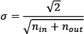 .
.
TensorFlow supports Xavier initialization in both uniform and normal distributions of weights.
For more information about Glorot and Bengio's initialization scheme, including the mathematical derivation and proof, read their original paper (Understanding the difficulty of deep feedforward neural networks, Xavier Glorot and Yoshua Bengio, 2010), which is freely available at http://proceedings.mlr.press/v9/glorot10a/glorot10a.pdf.
Now, to put this into the context of a more practical use case, let's see how we can define a Variable inside the base tf.Module class. We will define two variables: a trainable one and a non-trainable one:
>>> class MyModule(tf.Module):
...     def __init__(self):
...         init = tf.keras.initializers.GlorotNormal()
...         self.w1 = tf.Variable(init(shape=(2, 3)),
...                               trainable=True)
...         self.w2 = tf.Variable(init(shape=(1, 2)),
...                               trainable=False)
>>> m = MyModule()
>>> print('All module variables:', [v.shape for v in m.variables])
All module variables: [TensorShape([2, 3]), TensorShape([1, 2])]
>>> print('Trainable variable:', [v.shape for v in
...                               m.trainable_variables])
Trainable variable: [TensorShape([2, 3])]
As you can see in this code example, subclassing the tf.Module class gives us direct access to all variables defined in a given object (here, an instance of our custom MyModule class) via the .variables attribute.
Finally, let's look at using variables inside a function decorated with tf.function. When we define a TensorFlow Variable inside a normal function (not decorated), we might expect that a new Variable will be created and initialized each time the function is called. However, tf.function will try to reuse the Variable based on tracing and graph creation. Therefore, TensorFlow does not allow the creation of a Variable inside a decorated function and, as a result, the following code will raise an error:
>>> @tf.function
... def f(x):
...     w = tf.Variable([1, 2, 3])
>>> f([1])
ValueError: tf.function-decorated function tried to create variables on non-first call.
One way to avoid this problem is to define the Variable outside of the decorated function and use it inside the function:
>>> w = tf.Variable(tf.random.uniform((3, 3)))
>>> @tf.function
... def compute_z(x):
...     return tf.matmul(w, x)
>>> x = tf.constant([[1], [2], [3]], dtype=tf.float32)
>>> tf.print(compute_z(x))
Computing gradients via automatic differentiation and GradientTape
As you already know, optimizing NNs requires computing the gradients of the cost with respect to the NN weights. This is required for optimization algorithms such as stochastic gradient descent (SGD). In addition, gradients have other applications, such as diagnosing the network to find out why an NN model is making a particular prediction for a test example. Therefore, in this section, we will cover how to compute gradients of a computation with respect to some variables.
Computing the gradients of the loss with respect to trainable variables
TensorFlow supports automatic differentiation, which can be thought of as an implementation of the chain rule for computing gradients of nested functions. When we define a series of operations that results in some output or even intermediate tensors, TensorFlow provides a context for calculating gradients of these computed tensors with respect to its dependent nodes in the computation graph. In order to compute these gradients, we have to "record" the computations via tf.GradientTape.
Let's work with a simple example where we will compute ![]() and define the loss as the squared loss between the target and prediction,
and define the loss as the squared loss between the target and prediction, ![]() . In the more general case, where we may have multiple predictions and targets, we compute the loss as the sum of the squared error,
. In the more general case, where we may have multiple predictions and targets, we compute the loss as the sum of the squared error, ![]() . In order to implement this computation in TensorFlow, we will define the model parameters, w and b, as variables, and the input, x and y, as tensors. We will place the computation of z and the loss within the
. In order to implement this computation in TensorFlow, we will define the model parameters, w and b, as variables, and the input, x and y, as tensors. We will place the computation of z and the loss within the tf.GradientTape context:
>>> w = tf.Variable(1.0)
>>> b = tf.Variable(0.5)
>>> print(w.trainable, b.trainable)
True True
>>> x = tf.convert_to_tensor([1.4])
>>> y = tf.convert_to_tensor([2.1])
>>> with tf.GradientTape() as tape:
...     z = tf.add(tf.multiply(w, x), b)
...     loss = tf.reduce_sum(tf.square(y – z))
>>> dloss_dw = tape.gradient(loss, w)
>>> tf.print('dL/dw:', dloss_dw)
dL/dw: -0.559999764
When computing the value z, we could think of the required operations, which we recorded to the "gradient tape," as a forward pass in an NN. We used tape.gradient to compute  . Since this is a very simple example, we can obtain the derivatives,
  , symbolically to verify that the computed gradients match the results we obtained in the previous code example:
# verifying the computed gradient
>>> tf.print(2*x*(w*x+b-y))
[-0.559999764]
Understanding automatic differentiation
Automatic differentiation represents a set of computational techniques for computing derivatives or gradients of arbitrary arithmetic operations. During this process, gradients of a computation (expressed as a series of operations) are obtained by accumulating the gradients through repeated applications of the chain rule. To better understand the concept behind automatic differentiation, let's consider a series of computations, ![]() , with input x and output y. This can be broken into a series of steps:
, with input x and output y. This can be broken into a series of steps:
The derivative ![]() can be computed in two different ways: forward accumulation, which starts with
can be computed in two different ways: forward accumulation, which starts with 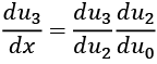 , and reverse accumulation, which starts with
  Note that TensorFlow uses the latter, reverse accumulation.
Computing gradients with respect to non-trainable tensors
tf.GradientTape automatically supports the gradients for trainable variables. However, for non-trainable variables and other Tensor objects, we need to add an additional modification to the GradientTape called tape.watch() to monitor those as well. For example, if we are interested in computing  , the code will be as follows:
>>> with tf.GradientTape() as tape:
...     tape.watch(x)
...     z = tf.add(tf.multiply(w, x), b)
...     loss = tf.reduce_sum(tf.square(y - z))
>>> dloss_dx = tape.gradient(loss, x)
>>> tf.print('dL/dx:', dloss_dx)
dL/dx: [-0.399999857]
Adversarial examples
Computing gradients of the loss with respect to the input example is used for generating adversarial examples (or adversarial attacks). In computer vision, adversarial examples are examples that are generated by adding some small imperceptible noise (or perturbations) to the input example, which results in a deep NN misclassifying them. Covering adversarial examples is beyond the scope of this book, but if you are interested, you can find the original paper by Christian Szegedy et al., titled Intriguing properties of neural networks, at https://arxiv.org/pdf/1312.6199.pdf.
Keeping resources for multiple gradient computations
When we monitor the computations in the context of tf.GradientTape, by default, the tape will keep the resources only for a single gradient computation. For instance, after calling tape.gradient() once, the resources will be released and the tape will be cleared. Hence, if we want to compute more than one gradient, for example, both  and
and  , we need to make the tape persistent:
>>> with tf.GradientTape(persistent=True) as tape:
...     z = tf.add(tf.multiply(w, x), b)
...     loss = tf.reduce_sum(tf.square(y – z))
>>> dloss_dw = tape.gradient(loss, w)
>>> tf.print('dL/dw:', dloss_dw)
dL/dw: -0.559999764
>>> dloss_db = tape.gradient(loss, b)
>>> tf.print('dL/db:', dloss_db)
dL/db: -0.399999857
However, keep in mind that this is only needed when we want to compute more than one gradient, as recording and keeping the gradient tape is less memory-efficient compared to releasing the memory after a single gradient computation. This is also why the default setting is persistent=False.
Finally, if we are computing gradients of a loss term with respect to the parameters of a model, we can define an optimizer and apply the gradients to optimize the model parameters using the tf.keras API, as follows:
>>> optimizer = tf.keras.optimizers.SGD()
>>> optimizer.apply_gradients(zip([dloss_dw, dloss_db], [w, b]))
>>> tf.print('Updated w:', w)
Updated w: 1.0056
>>> tf.print('Updated bias:', b)
Updated bias: 0.504
You will recall that the initial weight and bias unit were w = 1.0 and b = 0.5, and applying the gradients of the loss with respect to the model parameters changed the model parameters to w = 1.0056 and b = 0.504.
Simplifying implementations of common architectures via the Keras API
You have already seen some examples of building a feedforward NN model (for instance, a multilayer perceptron) and defining a sequence of layers using Keras' Sequential class. Before we look at different approaches for configuring those layers, let's briefly recap the basic steps by building a model with two densely (fully) connected layers:
>>> model = tf.keras.Sequential()
>>> model.add(tf.keras.layers.Dense(units=16, activation='relu'))
>>> model.add(tf.keras.layers.Dense(units=32, activation='relu'))
>>> ## late variable creation
>>> model.build(input_shape=(None, 4))
>>> model.summary()
Model: "sequential"
_________________________________________________________________
Layer (type)                 Output Shape              Param #
=================================================================
dense (Dense)                multiple                  80
_________________________________________________________________
dense_1 (Dense)              multiple                  544
=================================================================
Total params: 624
Trainable params: 624
Non-trainable params: 0
_________________________________________________________________
We specified the input shape with model.build(), instantiating the variables after defining the model for that particular shape. The number of parameters of each layer is displayed: ![]() for the first layer, and
for the first layer, and ![]() for the second layer. Once variables (or model parameters) are created, we can access both trainable and non-trainable variables as follows:
for the second layer. Once variables (or model parameters) are created, we can access both trainable and non-trainable variables as follows:
>>> ## printing variables of the model
>>> for v in model.variables:
...     print('{:20s}'.format(v.name), v.trainable, v.shape)
dense/kernel:0       True (4, 16)
dense/bias:0         True (16,)
dense_1/kernel:0     True (16, 32)
dense_1/bias:0       True (32,)
In this case, each layer has a weight matrix called kernel as well as a bias vector.
Next, let's configure these layers, for example, by applying different activation functions, variable initializers, or regularization methods to the parameters. A comprehensive and complete list of available options for these categories can be found in the official documentation:
- Choosing activation functions via
tf.keras.activations: https://www.tensorflow.org/versions/r2.0/api_docs/python/tf/keras/activations - Initializing the layer parameters via
tf.keras.initializers: https://www.tensorflow.org/versions/r2.0/api_docs/python/tf/keras/initializers - Applying regularization to the layer parameters (to prevent overfitting) via
tf.keras.regularizers: https://www.tensorflow.org/versions/r2.0/api_docs/python/tf/keras/regularizers
In the following code example, we will configure the first layer by specifying initializers for the kernel and bias variables. Then, we will configure the second layer by specifying an L1 regularizer for the kernel (weight matrix):
>>> model = tf.keras.Sequential()
>>> model.add(
...     tf.keras.layers.Dense(
...         units=16,
...         activation=tf.keras.activations.relu,
...         kernel_initializer=
...             tf.keras.initializers.glorot_uniform(),
...         bias_initializer=tf.keras.initializers.Constant(2.0)
...     ))
>>> model.add(
...     tf.keras.layers.Dense(
...         units=32,
...         activation=tf.keras.activations.sigmoid,
...         kernel_regularizer=tf.keras.regularizers.l1
...     ))
Furthermore, in addition to configuring the individual layers, we can also configure the model when we compile it. We can specify the type of optimizer and the loss function for training, as well as which metrics to use for reporting the performance on the training, validation, and test datasets. Again, a comprehensive list of all available options can be found in the official documentation:
- Optimizers via
tf.keras.optimizers: https://www.tensorflow.org/versions/r2.0/api_docs/python/tf/keras/optimizers - Loss functions via
tf.keras.losses: https://www.tensorflow.org/versions/r2.0/api_docs/python/tf/keras/losses - Performance metrics via
tf.keras.metrics: https://www.tensorflow.org/versions/r2.0/api_docs/python/tf/keras/metrics
Choosing a loss function
Regarding the choices for optimization algorithms, SGD and Adam are the most widely used methods. The choice of loss function depends on the task; for example, you might use mean square error loss for a regression problem.
The family of cross-entropy loss functions supplies the possible choices for classification tasks, which are extensively discussed in Chapter 15, Classifying Images with Deep Convolutional Neural Networks.
Furthermore, you can use the techniques you have learned from previous chapters (for example, techniques for model evaluation from Chapter 6, Learning Best Practices for Model Evaluation and Hyperparameter Tuning) combined with the appropriate metrics for the problem. For example, precision and recall, accuracy, area under the curve (AUC), and false negative and false positive scores are appropriate metrics for evaluating classification models.
In this example, we will compile the model using the SGD optimizer, cross-entropy loss for binary classification, and a specific list of metrics, including accuracy, precision, and recall:
>>> model.compile(
...     optimizer=tf.keras.optimizers.SGD(learning_rate=0.001),
...     loss=tf.keras.losses.BinaryCrossentropy(),
...     metrics=[tf.keras.metrics.Accuracy(),
...              tf.keras.metrics.Precision(),
...              tf.keras.metrics.Recall(),])
When we train this model by calling model.fit(...), the history of the loss and the specified metrics for evaluating training and validation performance (if a validation dataset is used) will be returned, which can be used to diagnose the learning behavior.
Next, we will look at a more practical example: solving the classic XOR classification problem using the Keras API. First, we will use the tf.keras.Sequential() class to build the model. Along the way, you will also learn about the capacity of a model for handling nonlinear decision boundaries. Then, we will cover other ways of building a model that will give us more flexibility and control over the layers of the network.
Solving an XOR classification problem
The XOR classification problem is a classic problem for analyzing the capacity of a model with regard to capturing the nonlinear decision boundary between two classes. We generate a toy dataset of 200 training examples with two features ![]() drawn from a uniform distribution between
drawn from a uniform distribution between ![]() . Then, we assign the ground truth label for training example i according to the following rule:
. Then, we assign the ground truth label for training example i according to the following rule:
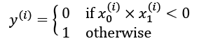
We will use half of the data (100 training examples) for training and the remaining half for validation. The code for generating the data and splitting it into the training and validation datasets is as follows:
>>> import tensorflow as tf
>>> import numpy as np
>>> import matplotlib.pyplot as plt
>>> tf.random.set_seed(1)
>>> np.random.seed(1)
>>> x = np.random.uniform(low=-1, high=1, size=(200, 2))
>>> y = np.ones(len(x))
>>> y[x[:, 0] * x[:, 1]<0] = 0
>>> x_train = x[:100, :]
>>> y_train = y[:100]
>>> x_valid = x[100:, :]
>>> y_valid = y[100:]
>>> fig = plt.figure(figsize=(6, 6))
>>> plt.plot(x[y==0, 0],
...          x[y==0, 1], 'o', alpha=0.75, markersize=10)
>>> plt.plot(x[y==1, 0],
...          x[y==1, 1], '<', alpha=0.75, markersize=10)
>>> plt.xlabel(r'$x_1$', size=15)
>>> plt.ylabel(r'$x_2$', size=15)
>>> plt.show()
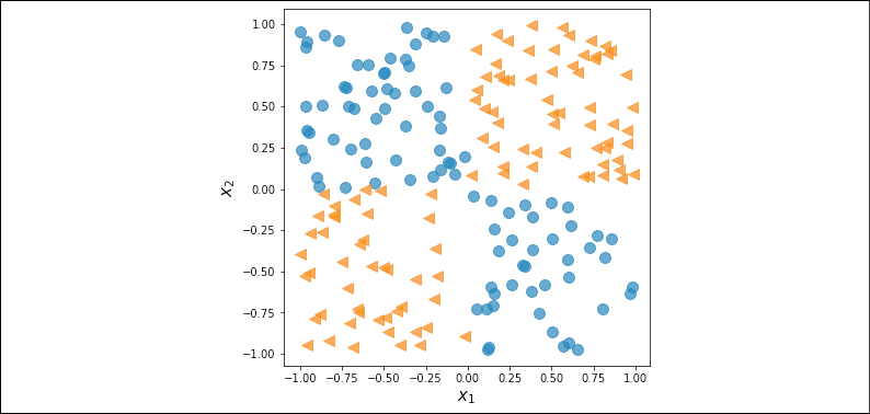
The code results in the following scatterplot of the training and validation examples, shown with different markers based on their class label:
In the previous subsection, we covered the essential tools that we need to implement a classifier in TensorFlow. We now need to decide what architecture we should choose for this task and dataset. As a general rule of thumb, the more layers we have, and the more neurons we have in each layer, the larger the capacity of the model will be. Here, the model capacity can be thought of as a measure of how readily the model can approximate complex functions. While having more parameters means the network can fit more complex functions, larger models are usually harder to train (and prone to overfitting). In practice, it is always a good idea to start with a simple model as a base line, for example, a single-layer NN like logistic regression:
>>> model = tf.keras.Sequential()
>>> model.add(tf.keras.layers.Dense(units=1,
...                                 input_shape=(2,),
...                                 activation='sigmoid'))
>>> model.summary()
Model: "sequential"
_________________________________________________________________
Layer (type)                 Output Shape              Param #
=================================================================
dense (Dense)                (None, 1)                 3
=================================================================
Total params: 3
Trainable params: 3
Non-trainable params: 0
_________________________________________________________________
The total size of the parameters for this simple logistic regression model is 3: a weight matrix (or kernel) of size ![]() and a bias vector of size 1. After defining the model, we will compile the model and train it for 200 epochs using a batch size of 2:
and a bias vector of size 1. After defining the model, we will compile the model and train it for 200 epochs using a batch size of 2:
>>> model.compile(optimizer=tf.keras.optimizers.SGD(),
...               loss=tf.keras.losses.BinaryCrossentropy(),
...               metrics=[tf.keras.metrics.BinaryAccuracy()])
>>> hist = model.fit(x_train, y_train,
...                  validation_data=(x_valid, y_valid),
...                  epochs=200, batch_size=2, verbose=0)
Notice that model.fit() returns a history of training epochs, which is useful for visual inspection after training. In the following code, we will plot the learning curves, including the training and validation loss, as well as their accuracies.
We will also use the MLxtend library to visualize the validation data and the decision boundary.
MLxtend can be installed via conda or pip as follows:
conda install mlxtend -c conda-forge
pip install mlxtend
The following code will plot the training performance along with the decision region bias:
>>> from mlxtend.plotting import plot_decision_regions
>>> history = hist.history
>>> fig = plt.figure(figsize=(16, 4))
>>> ax = fig.add_subplot(1, 3, 1)
>>> plt.plot(history['loss'], lw=4)
>>> plt.plot(history['val_loss'], lw=4)
>>> plt.legend(['Train loss', 'Validation loss'], fontsize=15)
>>> ax.set_xlabel('Epochs', size=15)
>>> ax = fig.add_subplot(1, 3, 2)
>>> plt.plot(history['binary_accuracy'], lw=4)
>>> plt.plot(history['val_binary_accuracy'], lw=4)
>>> plt.legend(['Train Acc.', 'Validation Acc.'], fontsize=15)
>>> ax.set_xlabel('Epochs', size=15)
>>> ax = fig.add_subplot(1, 3, 3)
>>> plot_decision_regions(X=x_valid, y=y_valid.astype(np.integer),
...                       clf=model)
>>> ax.set_xlabel(r'$x_1$', size=15)
>>> ax.xaxis.set_label_coords(1, -0.025)
>>> ax.set_ylabel(r'$x_2$', size=15)
>>> ax.yaxis.set_label_coords(-0.025, 1)
>>> plt.show()
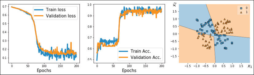
This results in the following figure, with three separate panels for the losses, accuracies, and the scatterplot of the validation examples, along with the decision boundary:

As you can see, a simple model with no hidden layer can only derive a linear decision boundary, which is unable to solve the XOR problem. As a consequence, we can observe that the loss terms for both the training and the validation datasets are very high, and the classification accuracy is very low.
In order to derive a nonlinear decision boundary, we can add one or more hidden layers connected via nonlinear activation functions. The universal approximation theorem states that a feedforward NN with a single hidden layer and a relatively large number of hidden units can approximate arbitrary continuous functions relatively well. Thus, one approach for tackling the XOR problem more satisfactorily is to add a hidden layer and compare different numbers of hidden units until we observe satisfactory results on the validation dataset. Adding more hidden units would correspond to increasing the width of a layer.
Alternatively, we can also add more hidden layers, which will make the model deeper. The advantage of making a network deeper rather than wider is that fewer parameters are required to achieve a comparable model capacity. However, a downside of deep (versus wide) models is that deep models are prone to vanishing and exploding gradients, which make them harder to train.
As an exercise, try adding one, two, three, and four hidden layers, each with four hidden units. In the following example, we will take a look at the results of a feedforward NN with three hidden layers:
>>> tf.random.set_seed(1)
>>> model = tf.keras.Sequential()
>>> model.add(tf.keras.layers.Dense(units=4, input_shape=(2,),
...                                 activation='relu'))
>>> model.add(tf.keras.layers.Dense(units=4, activation='relu'))
>>> model.add(tf.keras.layers.Dense(units=4, activation='relu'))
>>> model.add(tf.keras.layers.Dense(units=1, activation='sigmoid'))
>>> model.summary()
Model: "sequential_4"
_________________________________________________________________
Layer (type)                 Output Shape              Param #
=================================================================
dense_11 (Dense)             (None, 4)                 12
_________________________________________________________________
dense_12 (Dense)             (None, 4)                 20
_________________________________________________________________
dense_13 (Dense)             (None, 4)                 20
_________________________________________________________________
dense_14 (Dense)             (None, 1)                 5
=================================================================
Total params: 57
Trainable params: 57
Non-trainable params: 0
_________________________________________________________________
>>> ## compile:
>>> model.compile(optimizer=tf.keras.optimizers.SGD(),
...               loss=tf.keras.losses.BinaryCrossentropy(),
...               metrics=[tf.keras.metrics.BinaryAccuracy()])
>>> ## train:
>>> hist = model.fit(x_train, y_train,
...                  validation_data=(x_valid, y_valid),
...                  epochs=200, batch_size=2, verbose=0)
We can repeat the previous code for visualization, which produces the following:

Now, we can see that the model is able to derive a nonlinear decision boundary for this data, and the model reaches 100 percent accuracy on the training dataset. The validation dataset's accuracy is 95 percent, which indicates that the model is slightly overfitting.
Making model building more flexible with Keras' functional API
In the previous example, we used the Keras Sequential class to create a fully connected NN with multiple layers. This is a very common and convenient way of building models. However, it unfortunately doesn't allow us to create more complex models that have multiple input, output, or intermediate branches. That's where Keras' so-called functional API comes in handy.
To illustrate how the functional API can be used, we will implement the same architecture that we built using the objected-oriented (Sequential) approach in the previous section; however, this time, we will use the functional approach. In this approach, we first specify the input. Then, the hidden layers are constructed, with their outputs named h1, h2, and h3. For this problem, we use the output of each layer as the input to the succedent layer (note that if you are building more complex models that have multiple branches, this may not be the case, but it can still be done via the functional API). Finally, we specify the output as the final dense layer that receives h3 as input. The code for this is as follows:
>>> tf.random.set_seed(1)
>>> ## input layer:
>>> inputs = tf.keras.Input(shape=(2,))
>>> ## hidden layers
>>> h1 = tf.keras.layers.Dense(units=4, activation='relu')(inputs)
>>> h2 = tf.keras.layers.Dense(units=4, activation='relu')(h1)
>>> h3 = tf.keras.layers.Dense(units=4, activation='relu')(h2)
>>> ## output:
>>> outputs = tf.keras.layers.Dense(units=1, activation='sigmoid')(h3)
>>> ## construct a model:
>>> model = tf.keras.Model(inputs=inputs, outputs=outputs)
>>> model.summary()
Compiling and training this model is similar to what we did previously:
>>> ## compile:
>>> model.compile(
...     optimizer=tf.keras.optimizers.SGD(),
...     loss=tf.keras.losses.BinaryCrossentropy(),
...     metrics=[tf.keras.metrics.BinaryAccuracy()])
>>> ## train:
>>> hist = model.fit(
...     x_train, y_train,
...     validation_data=(x_valid, y_valid),
...     epochs=200, batch_size=2, verbose=0)
Implementing models based on Keras' Model class
An alternative way to build complex models is by subclassing tf.keras.Model. In this approach, we create a new class derived from tf.keras.Model and define the function, __init__(), as a constructor. The call() method is used to specify the forward pass. In the constructor function, __init__(), we define the layers as attributes of the class so that they can be accessed via the self reference attribute. Then, in the call() method, we specify how these layers are to be used in the forward pass of the NN. The code for defining a new class that implements the previous model is as follows:
>>> class MyModel(tf.keras.Model):
...     def __init__(self):
...         super(MyModel, self).__init__()
...         self.hidden_1 = tf.keras.layers.Dense(
...             units=4, activation='relu')
...         self.hidden_2 = tf.keras.layers.Dense(
...             units=4, activation='relu')
...         self.hidden_3 = tf.keras.layers.Dense(
...             units=4, activation='relu')
...         self.output_layer = tf.keras.layers.Dense(
...             units=1, activation='sigmoid')
...
...     def call(self, inputs):
...         h = self.hidden_1(inputs)
...         h = self.hidden_2(h)
...         h = self.hidden_3(h)
...         return self.output_layer(h)
Notice that we used the same output name, h, for all hidden layers. This makes the code more readable and easier to follow.
A model class derived from tf.keras.Model through subclassing inherits general model attributes, such as build(), compile(), and fit(). Therefore, once we define an instance of this new class, we can compile and train it like any other model built by Keras:
>>> tf.random.set_seed(1)
>>> model = MyModel()
>>> model.build(input_shape=(None, 2))
>>> model.summary()
>>> ## compile:
>>> model.compile(optimizer=tf.keras.optimizers.SGD(),
...               loss=tf.keras.losses.BinaryCrossentropy(),
...               metrics=[tf.keras.metrics.BinaryAccuracy()])
>>> ## train:
>>> hist = model.fit(x_train, y_train,
...                  validation_data=(x_valid, y_valid),
...                  epochs=200, batch_size=2, verbose=0)
Writing custom Keras layers
In cases where we want to define a new layer that is not already supported by Keras, we can define a new class derived from the tf.keras.layers.Layer class. This is especially useful when designing a new layer or customizing an existing layer.
To illustrate the concept of implementing custom layers, let's consider a simple example. Imagine we want to define a new linear layer that computes ![]() , where
, where ![]() refers to a random variable as a noise variable. To implement this computation, we define a new class as a subclass of
refers to a random variable as a noise variable. To implement this computation, we define a new class as a subclass of tf.keras.layers.Layer. For this new class, we have to define both the constructor __init__() method and the call() method. In the constructor, we define the variables and other required tensors for our customized layer. We have the option to create variables and initialize them in the constructor if the input_shape is given to the constructor. Alternatively, we can delay the variable initialization (for instance, if we do not know the exact input shape upfront) and delegate it to the build() method for late variable creation. In addition, we can define get_config() for serialization, which means that a model using our custom layer can be efficiently saved using TensorFlow's model saving and loading capabilities.
To look at a concrete example, we are going to define a new layer called NoisyLinear, which implements the computation ![]() , which was mentioned in the preceding paragraph:
, which was mentioned in the preceding paragraph:
>>> class NoisyLinear(tf.keras.layers.Layer):
...     def __init__(self, output_dim, noise_stddev=0.1, **kwargs):
...         self.output_dim = output_dim
...         self.noise_stddev = noise_stddev
...         super(NoisyLinear, self).__init__(**kwargs)
...
...     def build(self, input_shape):
...         self.w = self.add_weight(name='weights',
...                                  shape=(input_shape[1],
...                                         self.output_dim),
...                                  initializer='random_normal',
...                                  trainable=True)
...
...         self.b = self.add_weight(shape=(self.output_dim,),
...                                  initializer='zeros',
...                                  trainable=True)
...
...     def call(self, inputs, training=False):
...         if training:
...             batch = tf.shape(inputs)[0]
...             dim = tf.shape(inputs)[1]
...             noise = tf.random.normal(shape=(batch, dim),
...                                      mean=0.0,
...                                      stddev=self.noise_stddev)
...
...             noisy_inputs = tf.add(inputs, noise)
...         else:
...             noisy_inputs = inputs
...         z = tf.matmul(noisy_inputs, self.w) + self.b
...         return tf.keras.activations.relu(z)
...
...     def get_config(self):
...         config = super(NoisyLinear, self).get_config()
...         config.update({'output_dim': self.output_dim,
...                        'noise_stddev': self.noise_stddev})
...         return config
In the constructor, we have added an argument, noise_stddev, to specify the standard deviation for the distribution of ![]() , which is sampled from a Gaussian distribution. Furthermore, notice that in the
, which is sampled from a Gaussian distribution. Furthermore, notice that in the call() method, we have used an additional argument, training=False. In the context of Keras, the training argument is a special Boolean argument that distinguishes whether a model or layer is used during training (for example, via fit()) or only for prediction (for example, via predict(); this is sometimes also called "inference" or evaluation). One of the main differences between training and prediction is that during prediction, we do not require gradients. Also, there are certain methods that behave differently in training and prediction modes. You will encounter an example of such a method, Dropout, in the upcoming chapters. In the previous code snippet, we also specified that the random vector, ![]() , was to be generated and added to the input during training only and not used for inference or evaluation.
, was to be generated and added to the input during training only and not used for inference or evaluation.
Before we go a step further and use our custom NoisyLinear layer in a model, let's test it in the context of a simple example.
In the following code, we will define a new instance of this layer, initialize it by calling .build(), and execute it on an input tensor. Then, we will serialize it via .get_config() and restore the serialized object via .from_config():
>>> tf.random.set_seed(1)
>>> noisy_layer = NoisyLinear(4)
>>> noisy_layer.build(input_shape=(None, 4))
>>> x = tf.zeros(shape=(1, 4))
>>> tf.print(noisy_layer(x, training=True))
[[0 0.00821428 0 0]]
>>> ## re-building from config:
>>> config = noisy_layer.get_config()
>>> new_layer = NoisyLinear.from_config(config)
>>> tf.print(new_layer(x, training=True))
[[0 0.0108502861 0 0]]
In the previous code snippet, we called the layer two times on the same input tensor. However, note that the outputs differ because the NoisyLinear layer added random noise to the input tensor.
Now, let's create a new model similar to the previous one for solving the XOR classification task. As before, we will use Keras' Sequential class, but this time, we will use our NoisyLinear layer as the first hidden layer of the multilayer perceptron. The code is as follows:
>>> tf.random.set_seed(1)
>>> model = tf.keras.Sequential([
...     NoisyLinear(4, noise_stddev=0.1),
...     tf.keras.layers.Dense(units=4, activation='relu'),
...     tf.keras.layers.Dense(units=4, activation='relu'),
...     tf.keras.layers.Dense(units=1, activation='sigmoid')])
>>> model.build(input_shape=(None, 2))
>>> model.summary()
>>> ## compile:
>>> model.compile(optimizer=tf.keras.optimizers.SGD(),
...               loss=tf.keras.losses.BinaryCrossentropy(),
...               metrics=[tf.keras.metrics.BinaryAccuracy()])
>>> ## train:
>>> hist = model.fit(x_train, y_train,
...                  validation_data=(x_valid, y_valid),
...                  epochs=200, batch_size=2,
...                  verbose=0)
>>> ## Plotting
>>> history = hist.history
>>> fig = plt.figure(figsize=(16, 4))
>>> ax = fig.add_subplot(1, 3, 1)
>>> plt.plot(history['loss'], lw=4)
>>> plt.plot(history['val_loss'], lw=4)
>>> plt.legend(['Train loss', 'Validation loss'], fontsize=15)
>>> ax.set_xlabel('Epochs', size=15)
>>> ax = fig.add_subplot(1, 3, 2)
>>> plt.plot(history['binary_accuracy'], lw=4)
>>> plt.plot(history['val_binary_accuracy'], lw=4)
>>> plt.legend(['Train Acc.', 'Validation Acc.'], fontsize=15)
>>> ax.set_xlabel('Epochs', size=15)
>>> ax = fig.add_subplot(1, 3, 3)
>>> plot_decision_regions(X=x_valid, y=y_valid.astype(np.integer),
...                       clf=model)
>>> ax.set_xlabel(r'$x_1$', size=15)
>>> ax.xaxis.set_label_coords(1, -0.025)
>>> ax.set_ylabel(r'$x_2$', size=15)
>>> ax.yaxis.set_label_coords(-0.025, 1)
>>> plt.show()
The resulting figure will be as follows:
Here, our goal was to learn how to define a new custom layer subclassed from tf.keras.layers.Layer and to use it as we would use any other standard Keras layer. Although, with this particular example, NoisyLinear did not help to improve the performance, please keep in mind that our objective was to mainly learn how to write a customized layer from scratch. In general, writing a new customized layer can be useful in other applications, for example, if you develop a new algorithm that depends on a new layer beyond the existing ones.
TensorFlow Estimators
So far, in this chapter, we have mostly focused on the low-level TensorFlow API. We used decorators to modify functions to compile the computational graphs explicitly for computational efficiency. Then, we worked with the Keras API and implemented feedforward NNs, to which we added customized layers. In this section, we will switch gears and work with TensorFlow Estimators. The tf.estimator API encapsulates the underlying steps in machine learning tasks, such as training, prediction (inference), and evaluation. Estimators are more encapsulated but also more scalable when compared to the previous approaches that we have covered in this chapter. Also, the tf.estimator API adds support for running models on multiple platforms without requiring major code changes, which makes them more suitable for the so-called "production phase" in industry applications. In addition, TensorFlow comes with a selection of off-the-shelf estimators for common machine learning and deep learning architectures that are useful for comparison studies, for example, to quickly assess whether a certain approach is applicable to a particular dataset or problem.
In the remaining sections of this chapter, you will learn how to use such pre-made Estimators and how to create an Estimator from an existing Keras model. One of the essential elements of Estimators is defining the feature columns as a mechanism for importing data into an Estimator-based model, which we will cover in the next section.
Working with feature columns
In machine learning and deep learning applications, we can encounter various different types of features: continuous, unordered categorical (nominal), and ordered categorical (ordinal). You will recall that in Chapter 4, Building Good Training Datasets – Data Preprocessing, we covered different types of features and learned how to handle each type. Note that while numeric data can be either continuous or discrete, in the context of the TensorFlow API, "numeric" data specifically refers to continuous data of the floating point type.
Sometimes, feature sets are comprised of a mixture of different feature types. While TensorFlow Estimators were designed to handle all these different types of features, we must specify how each feature should be interpreted by the Estimator. For example, consider a scenario with a set of seven different features, as shown in the following figure:

The features shown in the figure (model year, cylinders, displacement, horsepower, weight, acceleration, and origin) were obtained from the Auto MPG dataset, which is a common machine learning benchmark dataset for predicting the fuel efficiency of a car in miles per gallon (MPG). The full dataset and its description are available from UCI's machine learning repository at https://archive.ics.uci.edu/ml/datasets/auto+mpg.
We are going to treat five features from the Auto MPG dataset (number of cylinders, displacement, horsepower, weight, and acceleration) as "numeric" (here, continuous) features. The model year can be regarded as an ordered categorical (ordinal) feature. Lastly, the manufacturing origin can be regarded as an unordered categorical (nominal) feature with three possible discrete values, 1, 2, and 3, which correspond to the US, Europe, and Japan, respectively.
Let's first load the data and apply the necessary preprocessing steps, such as partitioning the dataset into training and test datasets, as well as standardizing the continuous features:
>>> import pandas as pd
>>> dataset_path = tf.keras.utils.get_file(
...     "auto-mpg.data",
...     ("http://archive.ics.uci.edu/ml/machine-learning"
...      "-databases/auto-mpg/auto-mpg.data"))
>>> column_names = [
...     'MPG', 'Cylinders', 'Displacement',
...     'Horsepower', 'Weight', 'Acceleration',
...     'ModelYear', 'Origin']
>>> df = pd.read_csv(dataset_path, names=column_names,
...                  na_values = '?', comment='	',
...                  sep=' ', skipinitialspace=True)
>>> ## drop the NA rows
>>> df = df.dropna()
>>> df = df.reset_index(drop=True)
>>> ## train/test splits:
>>> import sklearn
>>> import sklearn.model_selection
>>> df_train, df_test = sklearn.model_selection.train_test_split(
...    df, train_size=0.8)
>>> train_stats = df_train.describe().transpose()
>>> numeric_column_names = [
...     'Cylinders', 'Displacement',
...     'Horsepower', 'Weight',
...     'Acceleration']
>>> df_train_norm, df_test_norm = df_train.copy(), df_test.copy()
>>> for col_name in numeric_column_names:
...     mean = train_stats.loc[col_name, 'mean']
...     std  = train_stats.loc[col_name, 'std']
...     df_train_norm.loc[:, col_name] = (
...         df_train_norm.loc[:, col_name] - mean)/std
...     df_test_norm.loc[:, col_name] = (
...         df_test_norm.loc[:, col_name] - mean)/std
>>> df_train_norm.tail()
This results in the following:
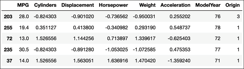
The pandas DataFrame that we created via the previous code snippet contains five columns with values of the type float. These columns will constitute the continuous features. In the following code, we will use TensorFlow's feature_column function to transform these continuous features into the feature column data structure that TensorFlow Estimators can work with:
>>> numeric_features = []
>>> for col_name in numeric_column_names:
...     numeric_features.append(
...         tf.feature_column.numeric_column(key=col_name))
Next, let's group the rather fine-grained model year information into buckets to simplify the learning task for the model that we are going to train later. Concretely, we are going to assign each car into one of four "year" buckets, as follows:
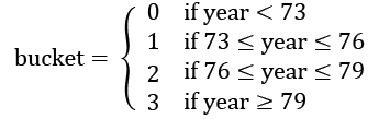
Note that the chosen intervals were selected arbitrarily to illustrate the concepts of "bucketing." In order to group the cars into these buckets, we will first define a numeric feature based on each original model year. Then, these numeric features will be passed to the bucketized_column function for which we will specify three interval cut-off values: [73, 76, 79]. The specified values include the right cut-off value. These cut-off values are used to specify half-closed intervals, for instance, ![]() ,
, ![]() ,
, ![]() , and
, and ![]() . The code is as follows:
. The code is as follows:
>>> feature_year = tf.feature_column.numeric_column(key='ModelYear')
>>> bucketized_features = []
>>> bucketized_features.append(
...     tf.feature_column.bucketized_column(
...         source_column=feature_year,
...         boundaries=[73, 76, 79]))
For consistency, we added this bucketized feature column to a Python list, even though the list consists of only one entry. In the following steps, we will merge this list with the lists made from other features, which will then be provided as input to the TensorFlow Estimator-based model.
Next, we will proceed with defining a list for the unordered categorical feature, Origin. In TensorFlow, there are different ways of creating a categorical feature column. If the data contains the category names (for example, in string format like "US," "Europe," and "Japan"), then we can use tf.feature_column.categorical_column_with_vocabulary_list and provide a list of unique, possible category names as input. If the list of possible categories is too large, for example, in a typical text analysis context, then we can use tf.feature_column.categorical_column_with_vocabulary_file instead. When using this function, we simply provide a file that contains all the categories/words so that we do not have to store a list of all possible words in memory. Moreover, if the features are already associated with an index of categories in the range [0, num_categories), then we can use the tf.feature_column.categorical_column_with_identity function. However, in this case, the feature Origin is given as integer values 1, 2, 3 (as opposed to 0, 1, 2), which does not match the requirement for categorical indexing, as it expects the indices to start from 0.
In the following code example, we will proceed with the vocabulary list:
>>> feature_origin = tf.feature_column.categorical_column_with_vocabulary_list(
...     key='Origin',
...     vocabulary_list=[1, 2, 3])
Certain Estimators, such as DNNClassifier and DNNRegressor, only accept so-called "dense columns." Therefore, the next step is to convert the existing categorical feature column to such a dense column. There are two ways to do this: using an embedding column via embedding_column or an indicator column via indicator_column. An indicator column converts the categorical indices to one-hot encoded vectors, for example, index 0 will be encoded as [1, 0, 0], index 1 will be encoded as [0, 1, 0], and so on. On the other hand, the embedding column maps each index to a vector of random number of the type float, which can be trained.
When the number of categories is large, using the embedding column with fewer dimensions than the number of categories can improve the performance. In the following code snippet, we will use the indicator column approach on the categorical feature in order to convert it into the dense format:
>>> categorical_indicator_features = []
>>> categorical_indicator_features.append(
...     tf.feature_column.indicator_column(feature_origin))
In this section, we have covered the most common approaches for creating feature columns that can be used with TensorFlow Estimators. However, there are several additional feature columns that we haven't discussed, including hashed columns and crossed columns. More information about these other feature columns can be found in the official TensorFlow documentation at https://www.tensorflow.org/versions/r2.0/api_docs/python/tf/feature_column.
Machine learning with pre-made Estimators
Now, after constructing the mandatory feature columns, we can finally utilize TensorFlow's Estimators. Using pre-made Estimators can be summarized in four steps:
- Define an input function for data loading
- Convert the dataset into feature columns
- Instantiate an Estimator (use a pre-made Estimator or create a new one, for example, by converting a Keras model into an Estimator)
- Use the Estimator methods
train(),evaluate(), andpredict()
Continuing with the Auto MPG example from the previous section, we will apply these four steps to illustrate how we can use Estimators in practice. For the first step, we need to define a function that processes the data and returns a TensorFlow dataset consisting of a tuple that contains the input features and the labels (ground truth MPG values). Note that the features must be in a dictionary format, and the keys of the dictionary must match the feature columns' names.
Starting with the first step, we will define the input function for the training data as follows:
>>> def train_input_fn(df_train, batch_size=8):
...     df = df_train.copy()
...     train_x, train_y = df, df.pop('MPG')
...     dataset = tf.data.Dataset.from_tensor_slices(
...         (dict(train_x), train_y))
...
...     # shuffle, repeat, and batch the examples.
...     return dataset.shuffle(1000).repeat().batch(batch_size)
Notice that we used dict(train_x) in this function to convert the pandas DataFrame object into a Python dictionary. Let's load a batch from this dataset to see how it looks:
>>> ds = train_input_fn(df_train_norm)
>>> batch = next(iter(ds))
>>> print('Keys:', batch[0].keys())
Keys: dict_keys(['Cylinders', 'Displacement', 'Horsepower', 'Weight', 'Acceleration', 'ModelYear', 'Origin'])
>>> print('Batch Model Years:', batch[0]['ModelYear'])
Batch Model Years: tf.Tensor([74 71 81 72 82 81 70 74], shape=(8,), dtype=int32)
We also need to define an input function for the test dataset that will be used for evaluation after model training:
>>> def eval_input_fn(df_test, batch_size=8):
...     df = df_test.copy()
...     test_x, test_y = df, df.pop('MPG')
...     dataset = tf.data.Dataset.from_tensor_slices(
...         (dict(test_x), test_y))
...     return dataset.batch(batch_size)
Now, moving on to step 2, we need to define the feature columns. We have already defined a list containing the continuous features, a list for the bucketized feature column, and a list for the categorical feature column. We can now concatenate these individual lists to a single list containing all feature columns:
>>> all_feature_columns = (
...     numeric_features +
...     bucketized_features +
...     categorical_indicator_features)
For step 3, we need to instantiate a new Estimator. Since predicting MPG values is a typical regression problem, we will use tf.estimator.DNNRegressor. When instantiating the regression Estimator, we will provide the list of feature columns and specify the number of hidden units that we want to have in each hidden layer using the argument hidden_units. Here, we will use two hidden layers, where the first hidden layer has 32 units and the second hidden layer has 10 units:
>>> regressor = tf.estimator.DNNRegressor(
...     feature_columns=all_feature_columns,
...     hidden_units=[32, 10],
...     model_dir='models/autompg-dnnregressor/')
The other argument, model_dir, that we have provided specifies the directory for saving model parameters. One of the advantages of Estimators is that they automatically checkpoint the model during training, so that in case the training of the model crashes for an unexpected reason (like power failure), we can easily load the last saved checkpoint and continue training from there. The checkpoints will also be saved in the directory specified by model_dir. If we do not specify the model_dir argument, the Estimator will create a random temporary folder (for example, in the Linux operating system, a random folder in the /tmp/ directory will be created), which will be used for this purpose.
After these three basic setup steps, we can finally use the Estimator for training, evaluation, and, eventually, prediction. The regressor can be trained by calling the train() method, for which we require the previously defined input function:
>>> EPOCHS = 1000
>>> BATCH_SIZE = 8
>>> total_steps = EPOCHS * int(np.ceil(len(df_train) / BATCH_SIZE))
>>> print('Training Steps:', total_steps)
Training Steps: 40000
>>> regressor.train(
...     input_fn=lambda:train_input_fn(
...         df_train_norm, batch_size=BATCH_SIZE),
...     steps=total_steps)
Calling .train() will automatically save the checkpoints during the training of the model. We can then reload the last checkpoint:
>>> reloaded_regressor = tf.estimator.DNNRegressor(
...     feature_columns=all_feature_columns,
...     hidden_units=[32, 10],
...     warm_start_from='models/autompg-dnnregressor/',
...     model_dir='models/autompg-dnnregressor/')
Then, in order to evaluate the predictive performance of the trained model, we can use the evaluate() method, as follows:
>>> eval_results = reloaded_regressor.evaluate(
...     input_fn=lambda:eval_input_fn(df_test_norm, batch_size=8))
>>> print('Average-Loss {:.4f}'.format(
...       eval_results['average_loss']))
Average-Loss 15.1866
Finally, to predict the target values on new data points, we can use the predict() method. For the purposes of this example, suppose that the test dataset represents a dataset of new, unlabeled data points in a real-world application.
Note that in a real-world prediction task, the input function will only need to return a dataset consisting of features, assuming that the labels are not available. Here, we will simply use the same input function that we used for evaluation to get the predictions for each example:
>>> pred_res = regressor.predict(
...     input_fn=lambda: eval_input_fn(
...         df_test_norm, batch_size=8))
>>> print(next(iter(pred_res)))
{'predictions': array([23.747658], dtype=float32)}
While the preceding code snippets conclude the illustration of the four steps that are required for using pre-made Estimators, for practice, let's take a look at another pre-made Estimator: the boosted tree regressor, tf.estimator.BoostedTreeRegressor. Since, the input functions and the feature columns are already built, we just need to repeat steps 3 and 4. For step 3, we will create an instance of BoostedTreeRegressor and configure it to have 200 trees.
Decision tree boosting
We already covered the ensemble algorithms, including boosting, in Chapter 7, Combining Different Models for Ensemble Learning. The boosted tree algorithm is a special family of boosting algorithms that is based on the optimization of an arbitrary loss function. Feel free to visit https://medium.com/mlreview/gradient-boosting-from-scratch-1e317ae4587d to learn more.
>>> boosted_tree = tf.estimator.BoostedTreesRegressor(
...     feature_columns=all_feature_columns,
...     n_batches_per_layer=20,
...     n_trees=200)
>>> boosted_tree.train(
...     input_fn=lambda:train_input_fn(
...         df_train_norm, batch_size=BATCH_SIZE))
>>> eval_results = boosted_tree.evaluate(
...     input_fn=lambda:eval_input_fn(
...         df_test_norm, batch_size=8))
>>> print('Average-Loss {:.4f}'.format(
...       eval_results['average_loss']))
Average-Loss 11.2609
As you can see, the boosted tree regressor achieves lower average loss than the DNNRegressor. For a small dataset like this, this is expected.
In this section, we covered the essential steps for using TensorFlow's Estimators for regression. In the next subsection, we will take a look at a typical classification example using Estimators.
Using Estimators for MNIST handwritten digit classification
For this classification problem, we are going to use the DNNClassifier Estimator provided by TensorFlow, which lets us implement a multilayer perceptron very conveniently. In the previous section, we covered the four essential steps for using the pre-made Estimators in detail, which we will need to repeat in this section. First, we are going to import the tensorflow_datasets (tfds) submodule, which we can use to load the MNIST dataset and specify the hyperparameters of the model.
Estimator API and graph issues
Since parts of TensorFlow 2.0 are still a bit rough around the edges, you may encounter the following issue when executing the next code block: RuntimeError: Graph is finalized and cannot be modified. Currently, there is no good solution for this issue, and a suggested workaround is to restart your Python, IPython, or Jupyter Notebook session before executing the next code block.
The setup step includes loading the dataset and specifying hyperparameters (BUFFER_SIZE for shuffling the dataset, BATCH_SIZE for the size of mini-batches, and the number of training epochs):
>>> import tensorflow_datasets as tfds
>>> import tensorflow as tf
>>> import numpy as np
>>> BUFFER_SIZE = 10000
>>> BATCH_SIZE = 64
>>> NUM_EPOCHS = 20
>>> steps_per_epoch = np.ceil(60000 / BATCH_SIZE)
Note that steps_per_epoch determines the number of iterations in each epoch, which is needed for infinitely repeated datasets (as discussed in Chapter 13, Parallelizing Neural Network Training with TensorFlow. Next, we will define a helper function that will preprocess the input image and its label.
Since the input image is originally of the type 'uint8' (in the range [0, 255]), we will use tf.image.convert_image_dtype() to convert its type to tf.float32 (and thereby, within the range [0, 1]):
>>> def preprocess(item):
...     image = item['image']
...     label = item['label']
...     image = tf.image.convert_image_dtype(
...         image, tf.float32)
...     image = tf.reshape(image, (-1,))
...
...     return {'image-pixels':image}, label[..., tf.newaxis]
Step 1: Define two input functions (one for training and one for evaluation):
>>> ## Step 1: Define the input functions
>>> def train_input_fn():
...     datasets = tfds.load(name='mnist')
...     mnist_train = datasets['train']
...
...     dataset = mnist_train.map(preprocess)
...     dataset = dataset.shuffle(BUFFER_SIZE)
...     dataset = dataset.batch(BATCH_SIZE)
...     return dataset.repeat()
>>> def eval_input_fn():
...     datasets = tfds.load(name='mnist')
...     mnist_test = datasets['test']
...     dataset = mnist_test.map(preprocess).batch(BATCH_SIZE)
...     return dataset
Notice that the dictionary of features has only one key, 'image-pixels'. We will use this key in the next step.
Step 2: Define the feature columns:
>>> ## Step 2: feature columns
>>> image_feature_column = tf.feature_column.numeric_column(
...     key='image-pixels', shape=(28*28))
Note that here, we defined the feature columns of size 784 (that is, ![]() ), which is the size of the input MNIST images after they are flattened.
), which is the size of the input MNIST images after they are flattened.
Step 3: Create a new Estimator. Here, we specify two hidden layers: 32 units in the first hidden layer and 16 units in the second.
We also specify the number of classes (remember that MNIST consists of 10 different digits, 0-9) using the argument n_classes:
>>> ## Step 3: instantiate the estimator
>>> dnn_classifier = tf.estimator.DNNClassifier(
...     feature_columns=[image_feature_column],
...     hidden_units=[32, 16],
...     n_classes=10,
...     model_dir='models/mnist-dnn/')
Step 4: Use the Estimator for training, evaluation, and prediction:
>>> ## Step 4: train and evaluate
>>> dnn_classifier.train(
...     input_fn=train_input_fn,
...     steps=NUM_EPOCHS * steps_per_epoch)
>>> eval_result = dnn_classifier.evaluate(
...     input_fn=eval_input_fn)
>>> print(eval_result)
{'accuracy': 0.8957, 'average_loss': 0.3876346, 'loss': 0.38815108, 'global_step': 18760}
So far, you have learned how to use pre-made Estimators and apply them for preliminary assessment to see, for example, whether an existing model is suitable for a particular problem. Besides using pre-made Estimators, we can also create an Estimator by converting a Keras model to an Estimator, which we will do in the next subsection.
Creating a custom Estimator from an existing Keras model
Converting a Keras model to an Estimator is useful in academia as well as industry for cases where you have developed a model and want to publish it or share the model with other members in your organization. Such a conversion allows us to access the strengths of Estimators, such as distributed training and automatic checkpointing. In addition, it will make it easy for others to use this model, and particularly to avoid confusions in interpreting the input features by specifying the feature columns and the input function.
To learn how we can create our own Estimator from a Keras model, we will work with the previous XOR problem. First, we will regenerate the data and split it into training and validation datasets:
>>> tf.random.set_seed(1)
>>> np.random.seed(1)
>>> ## Create the data
>>> x = np.random.uniform(low=-1, high=1, size=(200, 2))
>>> y = np.ones(len(x))
>>> y[x[:, 0] * x[:, 1]<0] = 0
>>> x_train = x[:100, :]
>>> y_train = y[:100]
>>> x_valid = x[100:, :]
>>> y_valid = y[100:]
Let's also build a Keras model that we want to convert to an Estimator later. We will define the model using the Sequential class as before. This time, we will also add an input layer defined as tf.keras.layers.Input to give a name to the input to this model:
>>> model = tf.keras.Sequential([
...     tf.keras.layers.Input(shape=(2,), name='input-features'),
...     tf.keras.layers.Dense(units=4, activation='relu'),
...     tf.keras.layers.Dense(units=4, activation='relu'),
...     tf.keras.layers.Dense(units=4, activation='relu'),
...     tf.keras.layers.Dense(1, activation='sigmoid')
... ])
Next, we will go through the four steps that we described in the previous subsection. Steps 1, 2, and 4 will be the same as the ones we used with the pre-made estimators. Note that the key name for the input features that we use in steps 1 and 2 must match with what we defined in the input layer of our model. The code is as follows:
>>> ## Step 1: Define the input functions
>>> def train_input_fn(x_train, y_train, batch_size=8):
...     dataset = tf.data.Dataset.from_tensor_slices(
...         ({'input-features':x_train}, y_train.reshape(-1, 1)))
...
...     # shuffle, repeat, and batch the examples.
...     return dataset.shuffle(100).repeat().batch(batch_size)
>>> def eval_input_fn(x_test, y_test=None, batch_size=8):
...     if y_test is None:
...         dataset = tf.data.Dataset.from_tensor_slices(
...             {'input-features':x_test})
...     else:
...         dataset = tf.data.Dataset.from_tensor_slices(
...             ({'input-features':x_test}, y_test.reshape(-1, 1)))
...
...
...     # shuffle, repeat, and batch the examples.
...     return dataset.batch(batch_size)
>>> ## Step 2: Define the feature columns
>>> features = [
...     tf.feature_column.numeric_column(
...         key='input-features:', shape=(2,))
... ]
For step 3, we will convert the model to an Estimator using tf.keras.estimator.model_to_estimator instead of instantiating one of the pre-made Estimators. Before converting the model, we first need to compile it:
>>> model.compile(optimizer=tf.keras.optimizers.SGD(),
...               loss=tf.keras.losses.BinaryCrossentropy(),
...               metrics=[tf.keras.metrics.BinaryAccuracy()])
>>> my_estimator = tf.keras.estimator.model_to_estimator(
...     keras_model=model,
...     model_dir='models/estimator-for-XOR/')
Finally, in step 4, we can train our model using the Estimator and evaluate it on the validation dataset:
>>> ## Step 4: Use the estimator
>>> num_epochs = 200
>>> batch_size = 2
>>> steps_per_epoch = np.ceil(len(x_train) / batch_size)
>>> my_estimator.train(
...     input_fn=lambda: train_input_fn(x_train, y_train, batch_size),
...     steps=num_epochs * steps_per_epoch)
>>> my_estimator.evaluate(
...     input_fn=lambda: eval_input_fn(x_valid, y_valid, batch_size))
{'binary_accuracy': 0.96, 'loss': 0.081909806, 'global_step': 10000}
As you can see, converting a Keras model to an Estimator is very straightforward. Doing this allows us to easily benefit from the various Estimator strengths, such as distributed training and automatically saving the checkpoints during training.
Summary
In this chapter, we covered TensorFlow's most essential and useful features. We started by discussing the migration from TensorFlow v1.x to v2. In particular, we used TensorFlow's dynamic computation graph approach, the so-called eager execution mode, which makes implementing computations more convenient compared to using static graphs. We also covered the semantics of defining TensorFlow Variable objects as model parameters, annotating Python functions using the tf.function decorator to improve computational efficiency via graph compilation.
After we considered the concept of computing partial derivatives and gradients of arbitrary functions, we covered the Keras API in more detail. It provides us with a user-friendly interface for building more complex deep NN models. Finally, we utilized TensorFlow's tf.estimator API to provide a consistent interface that is typically preferred in production environments. We concluded this chapter by converting a Keras model into a custom Estimator.
Now that we have covered the core mechanics of TensorFlow, the next chapter will introduce the concept behind convolutional neural network (CNN) architectures for deep learning. CNNs are powerful models and have shown great performance in the field of computer vision.