In this chapter, we will make use of two of the first algorithmically described machine learning algorithms for classification: the perceptron and adaptive linear neurons. We will start by implementing a perceptron step by step in Python and training it to classify different flower species in the Iris dataset. This will help us to understand the concept of machine learning algorithms for classification and how they can be efficiently implemented in Python.

Discussing the basics of optimization using adaptive linear neurons will then lay the groundwork for using more sophisticated classifiers via the scikit-learn machine learning library in Chapter 3, A Tour of Machine Learning Classifiers Using scikit-learn.

The topics that we will cover in this chapter are as follows:

• Building an understanding of machine learning algorithms
• Using pandas, NumPy, and Matplotlib to read in, process, and visualize data
• Implementing linear classification algorithms in Python

Artificial neurons – a brief glimpse into the early history of machine learning

Before we discuss the perceptron and related algorithms in more detail, let's take a brief tour of the beginnings of machine learning. Trying to understand how the biological brain works, in order to design artificial intelligence (AI), Warren McCulloch and Walter Pitts published the first concept of a simplified brain cell, the so-called McCulloch-Pitts (MCP) neuron, in 1943 (A Logical Calculus of the Ideas Immanent in Nervous Activity, W. S. McCulloch and W. Pitts, Bulletin of Mathematical Biophysics, 5(4): 115-133, 1943). Biological neurons are interconnected nerve cells in the brain that are involved in the processing and transmitting of chemical and electrical signals, which is illustrated in the following figure:

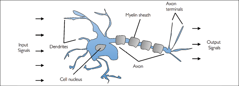
McCulloch and Pitts described such a nerve cell as a simple logic gate with binary outputs; multiple signals arrive at the dendrites, they are then integrated into the cell body, and, if the accumulated signal exceeds a certain threshold, an output signal is generated that will be passed on by the axon.

Only a few years later, Frank Rosenblatt published the first concept of the perceptron learning rule based on the MCP neuron model (The Perceptron: A Perceiving and Recognizing Automaton, F. Rosenblatt, Cornell Aeronautical Laboratory, 1957). With his perceptron rule, Rosenblatt proposed an algorithm that would automatically learn the optimal weight coefficients that would then be multiplied with the input features in order to make the decision of whether a neuron fires (transmits a signal) or not. In the context of supervised learning and classification, such an algorithm could then be used to predict whether a new data point belongs to one class or the other.

The formal definition of an artificial neuron

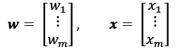
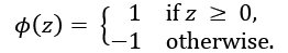
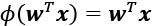
More formally, we can put the idea behind artificial neurons into the context of a binary classification task where we refer to our two classes as 1 (positive class) and –1 (negative class) for simplicity. We can then define a decision function () that takes a linear combination of certain input values, x, and a corresponding weight vector, w, where z is the so-called net input :

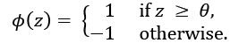
Now, if the net input of a particular example, , is greater than a defined threshold, , we predict class 1, and class –1 otherwise. In the perceptron algorithm, the decision function, , is a variant of a unit step function:

For simplicity, we can bring the threshold, , to the left side of the equation and define a weight-zero as and so that we write z in a more compact form:

And:

In machine learning literature, the negative threshold, or weight, , is usually called the bias unit.

Linear algebra basics: dot product and matrix transpose

In the following sections, we will often make use of basic notations from linear algebra. For example, we will abbreviate the sum of the products of the values in x and w using a vector dot product, whereas superscript T stands for transpose, which is an operation that transforms a column vector into a row vector and vice versa:

For example:

Furthermore, the transpose operation can also be applied to matrices to reflect it over its diagonal, for example:

Please note that the transpose operation is strictly only defined for matrices; however, in the context of machine learning, we refer to or matrices when we use the term "vector."

In this book, we will only use very basic concepts from linear algebra; however, if you need a quick refresher, please take a look at Zico Kolter's excellent Linear Algebra Review and Reference, which is freely available at http://www.cs.cmu.edu/~zkolter/course/linalg/linalg_notes.pdf.

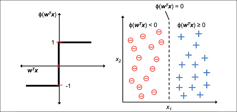
The following figure illustrates how the net input is squashed into a binary output (–1 or 1) by the decision function of the perceptron (left subfigure) and how it can be used to discriminate between two linearly separable classes (right subfigure):

The perceptron learning rule

The whole idea behind the MCP neuron and Rosenblatt's thresholded perceptron model is to use a reductionist approach to mimic how a single neuron in the brain works: it either fires or it doesn't. Thus, Rosenblatt's initial perceptron rule is fairly simple, and the perceptron algorithm can be summarized by the following steps:

1. Initialize the weights to 0 or small random numbers.
2. For each training example, :
   1. Compute the output value, .
   2. Update the weights.

Here, the output value is the class label predicted by the unit step function that we defined earlier, and the simultaneous update of each weight, , in the weight vector, w, can be more formally written as:

The update value for (or change in ), which we refer to as , is calculated by the perceptron learning rule as follows:

Where is the learning rate (typically a constant between 0.0 and 1.0), is the true class label of the ith training example, and is the predicted class label. It is important to note that all weights in the weight vector are being updated simultaneously, which means that we don't recompute the predicted label, , before all of the weights are updated via the respective update values, . Concretely, for a two-dimensional dataset, we would write the update as:

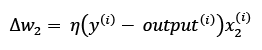
Before we implement the perceptron rule in Python, let's go through a simple thought experiment to illustrate how beautifully simple this learning rule really is. In the two scenarios where the perceptron predicts the class label correctly, the weights remain unchanged, since the update values are 0:

(1)

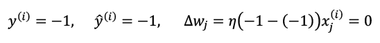
(2)

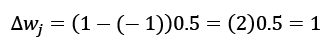
However, in the case of a wrong prediction, the weights are being pushed toward the direction of the positive or negative target class:

(3)

(4)

To get a better understanding of the multiplicative factor, , let's go through another simple example, where:

Let's assume that , and we misclassify this example as –1. In this case, we would increase the corresponding weight by 1 so that the net input, , would be more positive the next time we encounter this example, and thus be more likely to be above the threshold of the unit step function to classify the example as +1:

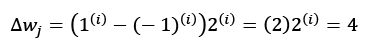
The weight update is proportional to the value of . For instance, if we have another example, , that is incorrectly classified as –1, we will push the decision boundary by an even larger extent to classify this example correctly the next time:

It is important to note that the convergence of the perceptron is only guaranteed if the two classes are linearly separable and the learning rate is sufficiently small (interested readers can find the mathematical proof in my lecture notes: https://sebastianraschka.com/pdf/lecture-notes/stat479ss19/L03_perceptron_slides.pdf.). If the two classes can't be separated by a linear decision boundary, we can set a maximum number of passes over the training dataset (epochs) and/or a threshold for the number of tolerated misclassifications—the perceptron would never stop updating the weights otherwise:

Now, before we jump into the implementation in the next section, what you just learned can be summarized in a simple diagram that illustrates the general concept of the perceptron:

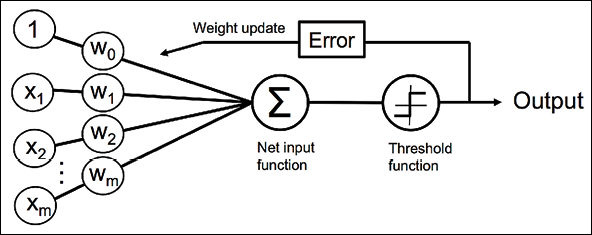
The preceding diagram illustrates how the perceptron receives the inputs of an example, x, and combines them with the weights, w, to compute the net input. The net input is then passed on to the threshold function, which generates a binary output of –1 or +1—the predicted class label of the example. During the learning phase, this output is used to calculate the error of the prediction and update the weights.

Implementing a perceptron learning algorithm in Python

In the previous section, we learned how Rosenblatt's perceptron rule works; let's now implement it in Python and apply it to the Iris dataset that we introduced in Chapter 1, Giving Computers the Ability to Learn from Data.

An object-oriented perceptron API

We will take an object-oriented approach to defining the perceptron interface as a Python class, which will allow us to initialize new Perceptron objects that can learn from data via a fit method, and make predictions via a separate predict method. As a convention, we append an underscore (_) to attributes that are not created upon the initialization of the object, but we do this by calling the object's other methods, for example, self.w_.

The following is the implementation of a perceptron in Python:

import numpy as np
class Perceptron(object):
    """Perceptron classifier.
    
    Parameters
    ------------
    eta : float
      Learning rate (between 0.0 and 1.0)
    n_iter : int
      Passes over the training dataset.
    random_state : int
      Random number generator seed for random weight 
      initialization.
    
    Attributes
    -----------
    w_ : 1d-array
      Weights after fitting.
    errors_ : list
      Number of misclassifications (updates) in each epoch.
    
    """
    def __init__(self, eta=0.01, n_iter=50, random_state=1):
        self.eta = eta
        self.n_iter = n_iter
        self.random_state = random_state
    
    def fit(self, X, y):
        """Fit training data.
        
        Parameters
        ----------
        X : {array-like}, shape = [n_examples, n_features]
          Training vectors, where n_examples is the number of 
          examples and n_features is the number of features.
        y : array-like, shape = [n_examples]
          Target values.
        
        Returns
        -------
        self : object
        
        """
        rgen = np.random.RandomState(self.random_state)
        self.w_ = rgen.normal(loc=0.0, scale=0.01,
                              size=1 + X.shape[1])
        self.errors_ = []
        
        for _ in range(self.n_iter):
            errors = 0
            for xi, target in zip(X, y):
                update = self.eta * (target - self.predict(xi))
                self.w_[1:] += update * xi
                self.w_[0] += update
                errors += int(update != 0.0)
            self.errors_.append(errors)
        return self
    
    def net_input(self, X):
        """Calculate net input"""
        return np.dot(X, self.w_[1:]) + self.w_[0]
    
    def predict(self, X):
        """Return class label after unit step"""
        return np.where(self.net_input(X) >= 0.0, 1, -1)

Using this perceptron implementation, we can now initialize new Perceptron objects with a given learning rate, eta, and the number of epochs, n_iter (passes over the training dataset).

Via the fit method, we initialize the weights in self.w_ to a vector, , where m stands for the number of dimensions (features) in the dataset, and we add 1 for the first element in this vector that represents the bias unit. Remember that the first element in this vector, self.w_[0], represents the so-called bias unit that we discussed earlier.

Also notice that this vector contains small random numbers drawn from a normal distribution with standard deviation 0.01 via rgen.normal(loc=0.0, scale=0.01, size=1 + X.shape[1]), where rgen is a NumPy random number generator that we seeded with a user-specified random seed so that we can reproduce previous results if desired.

It is important to keep in mind that we don't initialize the weights to zero because the learning rate, (eta), only has an effect on the classification outcome if the weights are initialized to non-zero values. If all the weights are initialized to zero, the learning rate parameter, eta, affects only the scale of the weight vector, not the direction. If you are familiar with trigonometry, consider a vector, , where the angle between and a vector, , would be exactly zero, as demonstrated by the following code snippet:

>>> v1 = np.array([1, 2, 3])
>>> v2 = 0.5 * v1
>>> np.arccos(v1.dot(v2) / (np.linalg.norm(v1) *
...           np.linalg.norm(v2)))
0.0

Here, np.arccos is the trigonometric inverse cosine, and np.linalg.norm is a function that computes the length of a vector (our decision to draw the random numbers from a random normal distribution—for example, instead of from a uniform distribution—and to use a standard deviation of 0.01 was arbitrary; remember, we are just interested in small random values to avoid the properties of all-zero vectors, as discussed earlier).

After the weights have been initialized, the fit method loops over all individual examples in the training dataset and updates the weights according to the perceptron learning rule that we discussed in the previous section.

The class labels are predicted by the predict method, which is called in the fit method during training to get the class label for the weight update; but predict can also be used to predict the class labels of new data after we have fitted our model. Furthermore, we also collect the number of misclassifications during each epoch in the self.errors_ list so that we can later analyze how well our perceptron performed during the training. The np.dot function that is used in the net_input method simply calculates the vector dot product, .

Training a perceptron model on the Iris dataset

To test our perceptron implementation, we will restrict the following analyses and examples in the remainder of this chapter to two feature variables (dimensions). Although the perceptron rule is not restricted to two dimensions, considering only two features, sepal length and petal length, will allow us to visualize the decision regions of the trained model in a scatter plot for learning purposes.

Note that we will also only consider two flower classes, Setosa and Versicolor, from the Iris dataset for practical reasons—remember, the perceptron is a binary classifier. However, the perceptron algorithm can be extended to multi-class classification—for example, the one-vs.-all (OvA) technique.

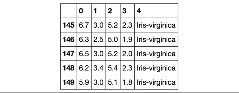
First, we will use the pandas library to load the Iris dataset directly from the UCI Machine Learning Repository into a DataFrame object and print the last five lines via the tail method to check that the data was loaded correctly:

>>> import os
>>> import pandas as pd
>>> s = os.path.join('https://archive.ics.uci.edu', 'ml',
...                  'machine-learning-databases',
...                  'iris','iris.data')
>>> print('URL:', s)
URL: https://archive.ics.uci.edu/ml/machine-learning-databases/iris/iris.data
>>> df = pd.read_csv(s,
...                  header=None,
...                  encoding='utf-8')
>>> df.tail()

df = pd.read_csv(
  'https://archive.ics.uci.edu/ml/'
  'machine-learning-databases/iris/iris.data',
  header=None, encoding='utf-8')

df = pd.read_csv(
  'your/local/path/to/iris.data',
  header=None, encoding='utf-8')

Next, we extract the first 100 class labels that correspond to the 50 Iris-setosa and 50 Iris-versicolor flowers and convert the class labels into the two integer class labels, 1 (versicolor) and -1 (setosa), that we assign to a vector, y, where the values method of a pandas DataFrame yields the corresponding NumPy representation.

Similarly, we extract the first feature column (sepal length) and the third feature column (petal length) of those 100 training examples and assign them to a feature matrix, X, which we can visualize via a two-dimensional scatterplot:

>>> import matplotlib.pyplot as plt
>>> import numpy as np
>>> # select setosa and versicolor
>>> y = df.iloc[0:100, 4].values
>>> y = np.where(y == 'Iris-setosa', -1, 1)
>>> # extract sepal length and petal length
>>> X = df.iloc[0:100, [0, 2]].values
>>> # plot data
>>> plt.scatter(X[:50, 0], X[:50, 1],
...             color='red', marker='o', label='setosa')
>>> plt.scatter(X[50:100, 0], X[50:100, 1],
...             color='blue', marker='x', label='versicolor')
>>> plt.xlabel('sepal length [cm]')
>>> plt.ylabel('petal length [cm]')
>>> plt.legend(loc='upper left')
>>> plt.show()

After executing the preceding code example, we should now see the following scatterplot:

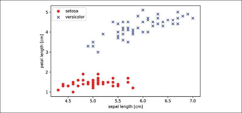
The preceding scatterplot shows the distribution of flower examples in the Iris dataset along the two feature axes: petal length and sepal length (measured in centimeters). In this two-dimensional feature subspace, we can see that a linear decision boundary should be sufficient to separate Setosa from Versicolor flowers.

Thus, a linear classifier such as the perceptron should be able to classify the flowers in this dataset perfectly.

Now, it's time to train our perceptron algorithm on the Iris data subset that we just extracted. Also, we will plot the misclassification error for each epoch to check whether the algorithm converged and found a decision boundary that separates the two Iris flower classes:

>>> ppn = Perceptron(eta=0.1, n_iter=10)
>>> ppn.fit(X, y)
>>> plt.plot(range(1, len(ppn.errors_) + 1),
...          ppn.errors_, marker='o')
>>> plt.xlabel('Epochs')
>>> plt.ylabel('Number of updates')
>>> plt.show()

After executing the preceding code, we should see the plot of the misclassification errors versus the number of epochs, as shown in the following graph:

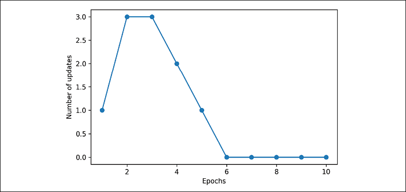
As we can see in the preceding plot, our perceptron converged after the sixth epoch and should now be able to classify the training examples perfectly. Let's implement a small convenience function to visualize the decision boundaries for two-dimensional datasets:

from matplotlib.colors import ListedColormap
def plot_decision_regions(X, y, classifier, resolution=0.02):
    # setup marker generator and color map
    markers = ('s', 'x', 'o', '^', 'v')
    colors = ('red', 'blue', 'lightgreen', 'gray', 'cyan')
    cmap = ListedColormap(colors[:len(np.unique(y))])
    
    # plot the decision surface
    x1_min, x1_max = X[:, 0].min() - 1, X[:, 0].max() + 1
    x2_min, x2_max = X[:, 1].min() - 1, X[:, 1].max() + 1
    xx1, xx2 = np.meshgrid(np.arange(x1_min, x1_max, resolution),
                           np.arange(x2_min, x2_max, resolution))
    Z = classifier.predict(np.array([xx1.ravel(), xx2.ravel()]).T)
    Z = Z.reshape(xx1.shape)
    plt.contourf(xx1, xx2, Z, alpha=0.3, cmap=cmap)
    plt.xlim(xx1.min(), xx1.max())
    plt.ylim(xx2.min(), xx2.max())
    
    # plot class examples
    for idx, cl in enumerate(np.unique(y)):
         plt.scatter(x=X[y == cl, 0],
                     y=X[y == cl, 1],
                     alpha=0.8,
                     c=colors[idx],
                     marker=markers[idx],
                     label=cl,
                     edgecolor='black')

First, we define a number of colors and markers and create a colormap from the list of colors via ListedColormap. Then, we determine the minimum and maximum values for the two features and use those feature vectors to create a pair of grid arrays, xx1 and xx2, via the NumPy meshgrid function. Since we trained our perceptron classifier on two feature dimensions, we need to flatten the grid arrays and create a matrix that has the same number of columns as the Iris training subset so that we can use the predict method to predict the class labels, Z, of the corresponding grid points.

After reshaping the predicted class labels, Z, into a grid with the same dimensions as xx1 and xx2, we can now draw a contour plot via Matplotlib's contourf function, which maps the different decision regions to different colors for each predicted class in the grid array:

>>> plot_decision_regions(X, y, classifier=ppn)
>>> plt.xlabel('sepal length [cm]')
>>> plt.ylabel('petal length [cm]')
>>> plt.legend(loc='upper left')
>>> plt.show()

After executing the preceding code example, we should now see a plot of the decision regions, as shown in the following figure:

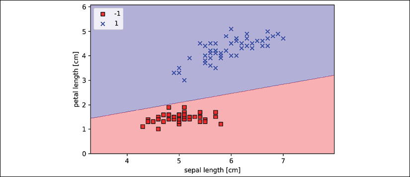
As we can see in the plot, the perceptron learned a decision boundary that is able to classify all flower examples in the Iris training subset perfectly.

Adaptive linear neurons and the convergence of learning

In this section, we will take a look at another type of single-layer neural network (NN): ADAptive LInear NEuron (Adaline). Adaline was published by Bernard Widrow and his doctoral student Tedd Hoff only a few years after Rosenblatt's perceptron algorithm, and it can be considered an improvement on the latter (An Adaptive "Adaline" Neuron Using Chemical "Memistors", Technical Report Number 1553-2, B. Widrow and others, Stanford Electron Labs, Stanford, CA, October 1960).

The Adaline algorithm is particularly interesting because it illustrates the key concepts of defining and minimizing continuous cost functions. This lays the groundwork for understanding more advanced machine learning algorithms for classification, such as logistic regression, support vector machines, and regression models, which we will discuss in future chapters.

The key difference between the Adaline rule (also known as the Widrow-Hoff rule) and Rosenblatt's perceptron is that the weights are updated based on a linear activation function rather than a unit step function like in the perceptron. In Adaline, this linear activation function, , is simply the identity function of the net input, so that:

While the linear activation function is used for learning the weights, we still use a threshold function to make the final prediction, which is similar to the unit step function that we covered earlier.

The main differences between the perceptron and Adaline algorithm are highlighted in the following figure:

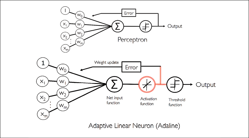
As the illustration indicates, the Adaline algorithm compares the true class labels with the linear activation function's continuous valued output to compute the model error and update the weights. In contrast, the perceptron compares the true class labels to the predicted class labels.

Minimizing cost functions with gradient descent

One of the key ingredients of supervised machine learning algorithms is a defined objective function that is to be optimized during the learning process. This objective function is often a cost function that we want to minimize. In the case of Adaline, we can define the cost function, J, to learn the weights as the sum of squared errors (SSE) between the calculated outcome and the true class label:

The term is just added for our convenience and will make it easier to derive the gradient of the cost or loss function with respect to the weight parameters, as we will see in the following paragraphs. The main advantage of this continuous linear activation function, in contrast to the unit step function, is that the cost function becomes differentiable. Another nice property of this cost function is that it is convex; thus, we can use a very simple yet powerful optimization algorithm called gradient descent to find the weights that minimize our cost function to classify the examples in the Iris dataset.

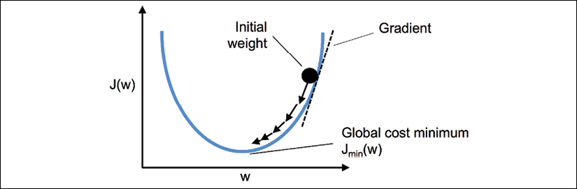
As illustrated in the following figure, we can describe the main idea behind gradient descent as climbing down a hill until a local or global cost minimum is reached. In each iteration, we take a step in the opposite direction of the gradient, where the step size is determined by the value of the learning rate, as well as the slope of the gradient:

Using gradient descent, we can now update the weights by taking a step in the opposite direction of the gradient, , of our cost function, :

The weight change, , is defined as the negative gradient multiplied by the learning rate, :

To compute the gradient of the cost function, we need to compute the partial derivative of the cost function with respect to each weight, :

So we can write the update of weight as:

Since we update all weights simultaneously, our Adaline learning rule becomes:

The squared error derivative

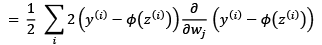
If you are familiar with calculus, the partial derivative of the SSE cost function with respect to the jth weight can be obtained as follows:

Although the Adaline learning rule looks identical to the perceptron rule, we should note that with is a real number and not an integer class label. Furthermore, the weight update is calculated based on all examples in the training dataset (instead of updating the weights incrementally after each training example), which is why this approach is also referred to as batch gradient descent.

Implementing Adaline in Python

Since the perceptron rule and Adaline are very similar, we will take the perceptron implementation that we defined earlier and change the fit method so that the weights are updated by minimizing the cost function via gradient descent:

class AdalineGD(object):
    """ADAptive LInear NEuron classifier.
    
    Parameters
    ------------
    eta : float
        Learning rate (between 0.0 and 1.0)
    n_iter : int
        Passes over the training dataset.
    random_state : int
        Random number generator seed for random weight initialization.
    
    Attributes
    -----------
    w_ : 1d-array
        Weights after fitting.
    cost_ : list
        Sum-of-squares cost function value in each epoch.
    
    """
    def __init__(self, eta=0.01, n_iter=50, random_state=1):
        self.eta = eta
        self.n_iter = n_iter
        self.random_state = random_state
    
    def fit(self, X, y):
        """ Fit training data.
        
        Parameters
        ----------
        X : {array-like}, shape = [n_examples, n_features]
            Training vectors, where n_examples
            is the number of examples and
            n_features is the number of features.
        y : array-like, shape = [n_examples]
            Target values.
        
        Returns
        -------
        self : object
        
        """
        rgen = np.random.RandomState(self.random_state)
        self.w_ = rgen.normal(loc=0.0, scale=0.01,
                              size=1 + X.shape[1])
        self.cost_ = []
        
        for i in range(self.n_iter):
            net_input = self.net_input(X)
            output = self.activation(net_input)
            errors = (y - output)
            self.w_[1:] += self.eta * X.T.dot(errors)
            self.w_[0] += self.eta * errors.sum()
            cost = (errors**2).sum() / 2.0
            self.cost_.append(cost)
        return self
    
    def net_input(self, X):
        """Calculate net input"""
        return np.dot(X, self.w_[1:]) + self.w_[0]
    
    def activation(self, X):
        """Compute linear activation"""
        return X
    
    def predict(self, X):
        """Return class label after unit step"""
        return np.where(self.activation(self.net_input(X))
                        >= 0.0, 1, -1)

Instead of updating the weights after evaluating each individual training example, as in the perceptron, we calculate the gradient based on the whole training dataset via self.eta * errors.sum() for the bias unit (zero-weight), and via self.eta * X.T.dot(errors) for the weights 1 to m, where X.T.dot(errors) is a matrix-vector multiplication between our feature matrix and the error vector.

Please note that the activation method has no effect in the code since it is simply an identity function. Here, we added the activation function (computed via the activation method) to illustrate the general concept with regard to how information flows through a single-layer NN: features from the input data, net input, activation, and output.

In the next chapter, we will learn about a logistic regression classifier that uses a non-identity, nonlinear activation function. We will see that a logistic regression model is closely related to Adaline, with the only difference being its activation and cost function.

Now, similar to the previous perceptron implementation, we collect the cost values in a self.cost_ list to check whether the algorithm converged after training.

Matrix multiplication

Performing a matrix multiplication is similar to calculating a vector dot-product where each row in the matrix is treated as a single row vector. This vectorized approach represents a more compact notation and results in a more efficient computation using NumPy. For example:

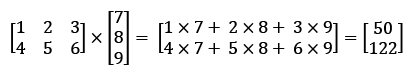
Please note that in the preceding equation, we are multiplying a matrix with a vector, which is mathematically not defined. However, remember that we use the convention that this preceding vector is regarded as a matrix.

In practice, it often requires some experimentation to find a good learning rate, , for optimal convergence. So, let's choose two different learning rates, and , to start with and plot the cost functions versus the number of epochs to see how well the Adaline implementation learns from the training data.

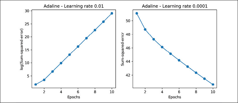
Let's now plot the cost against the number of epochs for the two different learning rates:

>>> fig, ax = plt.subplots(nrows=1, ncols=2, figsize=(10, 4))
>>> ada1 = AdalineGD(n_iter=10, eta=0.01).fit(X, y)
>>> ax[0].plot(range(1, len(ada1.cost_) + 1),
...            np.log10(ada1.cost_), marker='o')
>>> ax[0].set_xlabel('Epochs')
>>> ax[0].set_ylabel('log(Sum-squared-error)')
>>> ax[0].set_title('Adaline - Learning rate 0.01')
>>> ada2 = AdalineGD(n_iter=10, eta=0.0001).fit(X, y)
>>> ax[1].plot(range(1, len(ada2.cost_) + 1),
...            ada2.cost_, marker='o')
>>> ax[1].set_xlabel('Epochs')
>>> ax[1].set_ylabel('Sum-squared-error')
>>> ax[1].set_title('Adaline - Learning rate 0.0001')
>>> plt.show()

As we can see in the resulting cost-function plots, we encountered two different types of problem. The left chart shows what could happen if we choose a learning rate that is too large. Instead of minimizing the cost function, the error becomes larger in every epoch, because we overshoot the global minimum. On the other hand, we can see that the cost decreases on the right plot, but the chosen learning rate, , is so small that the algorithm would require a very large number of epochs to converge to the global cost minimum:

The following figure illustrates what might happen if we change the value of a particular weight parameter to minimize the cost function, J. The left subfigure illustrates the case of a well-chosen learning rate, where the cost decreases gradually, moving in the direction of the global minimum.

The subfigure on the right, however, illustrates what happens if we choose a learning rate that is too large—we overshoot the global minimum:

Improving gradient descent through feature scaling

Many machine learning algorithms that we will encounter throughout this book require some sort of feature scaling for optimal performance, which we will discuss in more detail in Chapter 3, A Tour of Machine Learning Classifiers Using scikit-learn, and Chapter 4, Building Good Training Datasets – Data Preprocessing.

Gradient descent is one of the many algorithms that benefit from feature scaling. In this section, we will use a feature scaling method called standardization, which gives our data the properties of a standard normal distribution: zero-mean and unit variance. This normalization procedure helps gradient descent learning to converge more quickly; however, it does not make the original dataset normally distributed. Standardization shifts the mean of each feature so that it is centered at zero and each feature has a standard deviation of 1 (unit variance). For instance, to standardize the jth feature, we can simply subtract the sample mean, , from every training example and divide it by its standard deviation, :

Here, is a vector consisting of the jth feature values of all training examples, n, and this standardization technique is applied to each feature, j, in our dataset.

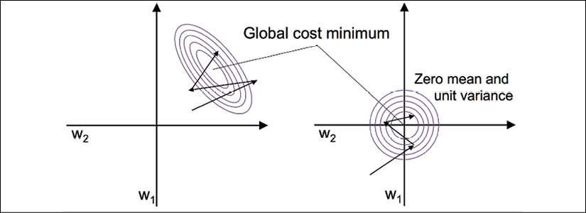
One of the reasons why standardization helps with gradient descent learning is that the optimizer has to go through fewer steps to find a good or optimal solution (the global cost minimum), as illustrated in the following figure, where the subfigures represent the cost surface as a function of two model weights in a two-dimensional classification problem:

Standardization can easily be achieved by using the built-in NumPy methods mean and std:

>>> X_std = np.copy(X)
>>> X_std[:,0] = (X[:,0] - X[:,0].mean()) / X[:,0].std()
>>> X_std[:,1] = (X[:,1] - X[:,1].mean()) / X[:,1].std()

After standardization, we will train Adaline again and we will see that it now converges after a small number of epochs using a learning rate of :

>>> ada_gd = AdalineGD(n_iter=15, eta=0.01)
>>> ada_gd.fit(X_std, y)
>>> plot_decision_regions(X_std, y, classifier=ada_gd)
>>> plt.title('Adaline - Gradient Descent')
>>> plt.xlabel('sepal length [standardized]')
>>> plt.ylabel('petal length [standardized]')
>>> plt.legend(loc='upper left')
>>> plt.tight_layout()
>>> plt.show()
>>> plt.plot(range(1, len(ada_gd.cost_) + 1),
...          ada_gd.cost_, marker='o')
>>> plt.xlabel('Epochs')
>>> plt.ylabel('Sum-squared-error')
>>> plt.tight_layout()
>>> plt.show()

After executing this code, we should see a figure of the decision regions, as well as a plot of the declining cost, as shown in the following figure:

As we can see in the plots, Adaline has now converged after training on the standardized features using a learning rate of . However, note that the SSE remains non-zero even though all flower examples were classified correctly.

Large-scale machine learning and stochastic gradient descent

In the previous section, we learned how to minimize a cost function by taking a step in the opposite direction of a cost gradient that is calculated from the whole training dataset; this is why this approach is sometimes also referred to as batch gradient descent. Now imagine that we have a very large dataset with millions of data points, which is not uncommon in many machine learning applications. Running batch gradient descent can be computationally quite costly in such scenarios, since we need to reevaluate the whole training dataset each time that we take one step toward the global minimum.

A popular alternative to the batch gradient descent algorithm is stochastic gradient descent (SGD), which is sometimes also called iterative or online gradient descent. Instead of updating the weights based on the sum of the accumulated errors over all training examples, :

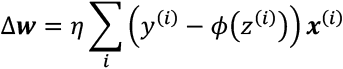
we update the weights incrementally for each training example:

Although SGD can be considered as an approximation of gradient descent, it typically reaches convergence much faster because of the more frequent weight updates. Since each gradient is calculated based on a single training example, the error surface is noisier than in gradient descent, which can also have the advantage that SGD can escape shallow local minima more readily if we are working with nonlinear cost functions, as we will see later in Chapter 12, Implementing a Multilayer Artificial Neural Network from Scratch. To obtain satisfying results via SGD, it is important to present training data in a random order; also, we want to shuffle the training dataset for every epoch to prevent cycles.

Adjusting the learning rate during training

In SGD implementations, the fixed learning rate, , is often replaced by an adaptive learning rate that decreases over time, for example:

where and are constants. Note that SGD does not reach the global minimum but an area very close to it. And using an adaptive learning rate, we can achieve further annealing to the cost minimum.

Another advantage of SGD is that we can use it for online learning. In online learning, our model is trained on the fly as new training data arrives. This is especially useful if we are accumulating large amounts of data, for example, customer data in web applications. Using online learning, the system can immediately adapt to changes, and the training data can be discarded after updating the model if storage space is an issue.

Since we already implemented the Adaline learning rule using gradient descent, we only need to make a few adjustments to modify the learning algorithm to update the weights via SGD. Inside the fit method, we will now update the weights after each training example. Furthermore, we will implement an additional partial_fit method, which does not reinitialize the weights, for online learning. In order to check whether our algorithm converged after training, we will calculate the cost as the average cost of the training examples in each epoch. Furthermore, we will add an option to shuffle the training data before each epoch to avoid repetitive cycles when we are optimizing the cost function; via the random_state parameter, we allow the specification of a random seed for reproducibility:

class AdalineSGD(object):
    """ADAptive LInear NEuron classifier.
    
    Parameters
    ------------
    eta : float
        Learning rate (between 0.0 and 1.0)
    n_iter : int
        Passes over the training dataset.
    shuffle : bool (default: True)
        Shuffles training data every epoch if True to prevent 
        cycles.
    random_state : int
        Random number generator seed for random weight 
        initialization.
    
    
    Attributes
    -----------
    w_ : 1d-array
        Weights after fitting.
    cost_ : list
        Sum-of-squares cost function value averaged over all
        training examples in each epoch.
    
    
    """
    def __init__(self, eta=0.01, n_iter=10,
              shuffle=True, random_state=None):
        self.eta = eta
        self.n_iter = n_iter
        self.w_initialized = False
        self.shuffle = shuffle
        self.random_state = random_state
    
    def fit(self, X, y):
        """ Fit training data.
        
        Parameters
        ----------
        X : {array-like}, shape = [n_examples, n_features]
            Training vectors, where n_examples is the number of 
            examples and n_features is the number of features.
        y : array-like, shape = [n_examples]
            Target values.
        
        Returns
        -------
        self : object
        
        """
        self._initialize_weights(X.shape[1])
        self.cost_ = []
        for i in range(self.n_iter):
            if self.shuffle:
                X, y = self._shuffle(X, y)
            cost = []
            for xi, target in zip(X, y):
                cost.append(self._update_weights(xi, target))
            avg_cost = sum(cost) / len(y)
            self.cost_.append(avg_cost)
        return self
    
    def partial_fit(self, X, y):
        """Fit training data without reinitializing the weights"""
        if not self.w_initialized:
            self._initialize_weights(X.shape[1])
        if y.ravel().shape[0] > 1:
            for xi, target in zip(X, y):
                self._update_weights(xi, target)
        else:
            self._update_weights(X, y)
        return self
    
    def _shuffle(self, X, y):
        """Shuffle training data"""
        r = self.rgen.permutation(len(y))
        return X[r], y[r]
    
    def _initialize_weights(self, m):
        """Initialize weights to small random numbers"""
        self.rgen = np.random.RandomState(self.random_state)
        self.w_ = self.rgen.normal(loc=0.0, scale=0.01,
                                   size=1 + m)
        self.w_initialized = True
    
    def _update_weights(self, xi, target):
        """Apply Adaline learning rule to update the weights"""
        output = self.activation(self.net_input(xi))
        error = (target - output)
        self.w_[1:] += self.eta * xi.dot(error)
        self.w_[0] += self.eta * error
        cost = 0.5 * error**2
        return cost
    
    def net_input(self, X):
        """Calculate net input"""
        return np.dot(X, self.w_[1:]) + self.w_[0]
    
    def activation(self, X):
        """Compute linear activation"""
        return X
    
    def predict(self, X):
        """Return class label after unit step"""
        return np.where(self.activation(self.net_input(X))
                        >= 0.0, 1, -1)

The _shuffle method that we are now using in the AdalineSGD classifier works as follows: via the permutation function in np.random, we generate a random sequence of unique numbers in the range 0 to 100. Those numbers can then be used as indices to shuffle our feature matrix and class label vector.

We can then use the fit method to train the AdalineSGD classifier and use our plot_decision_regions to plot our training results:

>>> ada_sgd = AdalineSGD(n_iter=15, eta=0.01, random_state=1)
>>> ada_sgd.fit(X_std, y)
>>> plot_decision_regions(X_std, y, classifier=ada_sgd)
>>> plt.title('Adaline - Stochastic Gradient Descent')
>>> plt.xlabel('sepal length [standardized]')
>>> plt.ylabel('petal length [standardized]')
>>> plt.legend(loc='upper left')
>>> plt.tight_layout()
>>> plt.show()
>>> plt.plot(range(1, len(ada_sgd.cost_) + 1), ada_sgd.cost_,
...          marker='o')
>>> plt.xlabel('Epochs')
>>> plt.ylabel('Average Cost')
>>> plt.tight_layout()
>>> plt.show()

The two plots that we obtain from executing the preceding code example are shown in the following figure:

As you can see, the average cost goes down pretty quickly, and the final decision boundary after 15 epochs looks similar to the batch gradient descent Adaline. If we want to update our model, for example, in an online learning scenario with streaming data, we could simply call the partial_fit method on individual training examples—for instance ada_sgd.partial_fit(X_std[0, :], y[0]).

Summary

In this chapter, we gained a good understanding of the basic concepts of linear classifiers for supervised learning. After we implemented a perceptron, we saw how we can train adaptive linear neurons efficiently via a vectorized implementation of gradient descent and online learning via SGD.

Now that we have seen how to implement simple classifiers in Python, we are ready to move on to the next chapter, where we will use the Python scikit-learn machine learning library to get access to more advanced and powerful machine learning classifiers, which are commonly used in academia as well as in industry.

The object-oriented approach that we used to implement the perceptron and Adaline algorithms will help with understanding the scikit-learn API, which is implemented based on the same core concepts that we used in this chapter: the fit and predict methods. Based on these core concepts, we will learn about logistic regression for modeling class probabilities and support vector machines for working with nonlinear decision boundaries. In addition, we will introduce a different class of supervised learning algorithms, tree-based algorithms, which are commonly combined into robust ensemble classifiers.