2.4 The Archimedes Approach
The first technique we will consider, which is attributed to the mathematician Archimedes, makes use of a many-sided polygon to approximate the circumference of a circle. Recall that pi is related to the circumference of a circle, C, by the equation

where r is the radius of the circle. Given a circle of radius 1, sometimes called a unit circle, this equation can be rearranged as simply

The Archimedes approach, shown in FIGURE 2.2, uses the distance around a polygon that is inscribed within a unit circle. By using a polygon with an increasing numbers of sides (and therefore decreasing side length), the total distance around the polygon will come closer and closer to the actual circumference of the circle. Does this sound familiar? Of course, no matter how large the number of sides, we will never truly match the actual circle with this method.
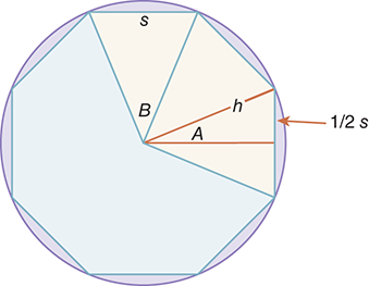
FIGURE 2.2 Developing the Archimedes approach using an eight-sided polygon.
Figure 2.2 shows more of the details that will be needed to understand how this approximation will work. If we assume that the polygon has n sides of length s, we can then focus our attention on a small slice of the polygon. In the orange triangle shown in the figure, the side labeled h will have a length of 1 because we are assuming a unit circle. The angle labeled B can be easily computed by remembering that there are 360 degrees in a circle. Thus, angle B is 360 ÷ n, and angle A is

In addition, we know that the highlighted triangle is a right triangle, so the side opposite angle A has a length of

Now we have to use a bit of trigonometry. In a right triangle (see FIGURE 2.3), the ratio of the opposite side to the long side (or hypotenuse) is equal to the sine of angle A. Because our triangle has a hypotenuse of length 1, we know that

will simply be equal to the sine of angle A. How do we compute the sine of angle A? The answer is to use the math library. As with sqrt earlier, the sin function (as well as all the other trigonometric relationships) is available once we import the math module.
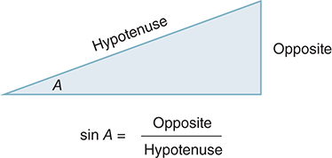
FIGURE 2.3 The sine of angle A.
2.4.1 The Python Implementation
SESSION 2.3 shows that it is possible to implement Archimedes’s algorithm by using the interactive Python environment. We can simply type in and evaluate statements that follow the steps outlined here. Note that the last step in Session 2.3 evaluates the value of pi as computed in the previous statement.
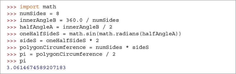
SESSION 2.3 The Archimedes approach: Interactive implementation
Before moving on, we should note one additional use of the math library. The sin function takes an angle and returns the ratio of the opposite side to the hypotenuse. However, it assumes that the angle will be in radians instead of degrees. When we compute angle B by dividing 360 by the number of sides, we get a value in degrees. Fortunately, the math library contains a function (called radians) that will convert a value in degrees to the equivalent value in radians. When we receive the result of the radians function, it becomes the parameter to the math.sin function.
2.4.2 Developing a Function to Compute Pi
What if we now want to change the number of sides and try the calculation again? Unfortunately, we would need to retype all the statements, because the calculations need to be redone. A better way to do this is to use abstraction.
Recall that abstraction allows us to think about a collection of steps as a logical group. In Python, we can define a function that not only serves as a name for a sequence of actions but also returns a value when it is called. We have already seen this type of behavior with the sqrt function. For example, when we call sqrt(16), it returns 4.0.
LISTING 2.1 shows the function definition template provided in Chapter 1 with one additional statement: return. The return statement causes two related actions. First, the expression contained in the statement is evaluated, producing a result object. Second, the function terminates immediately and the reference to the result object is returned to the calling statement. The bottom line is that the value of a function call is the value of the expression that is returned. It is important to realize that no matter where the return statement occurs, it will be the final statement performed because return causes the function to terminate. For this reason, return is typically the last statement in the function.
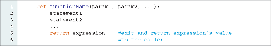
LISTING 2.1 Template for a function definition with return
In the case of the Archimedes pi approximation, we need to develop a function that has the behavior shown in FIGURE 2.4. This function will need one parameter—namely, the number of sides we wish to use in the polygon. The function will return the value of pi using the steps we developed earlier.
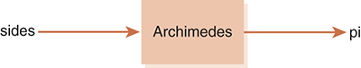
FIGURE 2.4 Abstraction with the Archimedes approximation.
LISTING 2.2 shows the archimedes function. As you look at each statement in this function, notice that the variable names match those we used as we worked through the previous problem- solving process. This practice makes it easier to see how the steps we discovered in the solution can be mapped into Python statements. In fact, one of the characteristics of a well-written function is the ability to read the code and see the underlying algorithm.
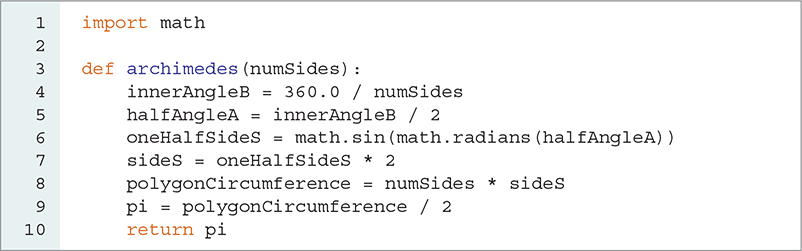
LISTING 2.2 Implementing the Archimedes approximation as a function
SESSION 2.4 shows how we can use the archimedes function. In the first evaluation, the name archimedes evaluates to a reference to a function object. The subsequent lines invoke the function while passing different numbers of sides. Note that the accuracy of the pi approximation gets better and better as we increase the number of sides in the polygon.
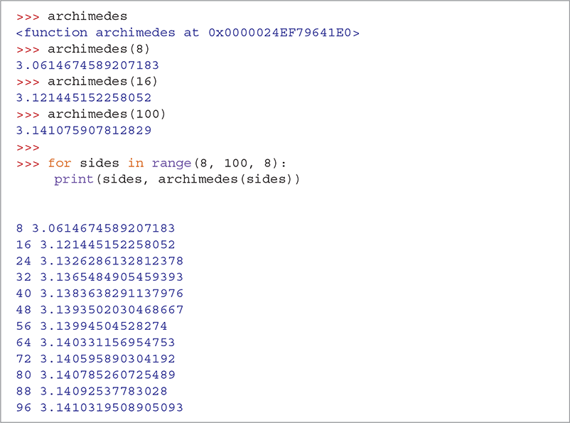
SESSION 2.4 Using the archimedes function
In the final code fragment of the session, we use a for statement to call the archimedes function repeatedly using a range construct to automatically provide different numbers of sides. Recall that range(8, 100, 8) will produce values for the variable sides starting at 8 and stopping at or before 99, increasing by 8 every time.
Session 2. 4 also includes another new Python function, print, which is shown in TABLE 2.1. Because the print function is a built-in Python function, you do not need to import a module to use the print function. This function accepts multiple parameters and prints the values of the parameters separated by a space, by default. In Session 2.4, we call the print function and pass it the number of sides used and the function call to our archimedes function. The print function then prints the number of sides, a space, and the result returned from the function in each iteration of the for loop.
TABLE 2.1 The |
|
|---|---|
| Function | Description |
print(param1, … ) |
Outputs each parameter value on the same line, separated by a space |