2.6 A Monte Carlo Simulation
Our final technique for approximating pi will make use of probability and random behavior. These types of solutions are often referred to as Monte Carlo simulations because they use features that are similar to “games of chance.” In other words, instead of knowing specifically what will happen during the simulation, a random element is introduced into the simulation so that it will behave differently each time.
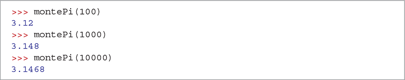
To set up our simulation, consider FIGURE 2.9. Pretend that we are looking at a dartboard in the shape of a square that is 2 units wide and 2 units high. A circle has been inscribed within the square so that the radius of the circle is 1 unit.
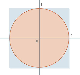
FIGURE 2.9 Setting up the Monte Carlo simulation.
Now assume that we cut out the upper-right quadrant of the square (see FIGURE 2.10). The result will be a square that is 1 unit high and 1 unit wide with a quarter-circle transcribed inside. This piece is what we will use to “play” our simulation. The area of the original square was 4 units. The area of the original circle was πr2 = π units since the circle had a radius of 1 unit. After we cut the upper-right quarter, the area of the quarter-circle is

and the area of the entire quarter square is 1.
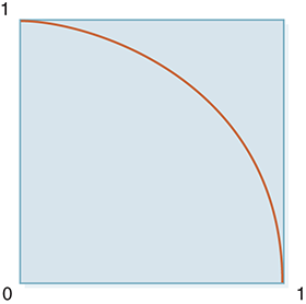
FIGURE 2.10 The upper-right quadrant.
The simulation will work by randomly “throwing darts” at the dartboard in Figure 2.10. We will assume that every dart hits the board but that the location of that strike will be random. It is easy to see that each dart will hit the square but some will land inside the quarter-circle. The number of darts that hit inside or outside the quarter-circle will be proportional to the areas of each. More specifically, the fraction of darts that land inside the quarter-circle will be equal to

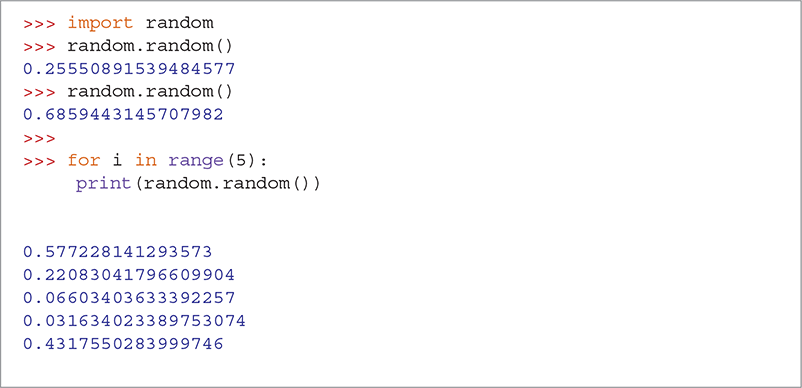
To implement this simulation, we will use the random module. You may find it useful to invoke the help command on this module to explore its functionality. For our purposes, we will use only the random function—a random number generator that returns a floating-point number between 0 and 1 each time it is called. TABLE 2.2 describes the random method, and SESSION 2.8 shows the random method in action. Note that because these numbers are randomly generated, your results will likely differ from the numbers shown in Session 2.8 and will likely differ each time you execute this code.
TABLE 2.2 The |
|
|---|---|
| Function | Description |
random() |
Returns a random number ranging from 0 up to, but not including, 1 |
SESSION 2.8 Exercising the random function
We will use random numbers to simulate the dart throw we described earlier. For each round of the simulation, we will randomly generate two numbers between 0 and 1, representing the position that each dart lands on our square. We can think of the board as having a horizontal axis and a vertical axis, both labeled between 0 and 1. If we let the first number represent the horizontal distance and the second represent the vertical distance, then the two numbers give us an (x, y) location for the point.
Our plan is to keep track of the number of points that land inside the quarter-circle and then use that number to compute our estimate for π. To do this, we need to be able to determine whether the location of the point is in the quarter-circle. Making this determination requires us to introduce a few new ideas.
2.6.1 Boolean Expressions
To solve the problem of deciding whether a point is inside or outside of the quarter-circle, we need to be able to ask a question. In computer science, questions are often referred to as Boolean expressions because the result of asking them is one of the two Boolean data values: True or False. These Boolean values are another primitive type in Python.
The easiest type of Boolean expression to write is one that compares the results of two expressions. To make this comparison, we use relational operators from mathematics such as equal to, less than, and greater than. TABLE 2.3 shows the relational operators and their meaning in Python.
TABLE 2.3 Relational Operators and Their Meaning |
|
|---|---|
| Relational Operator | Meaning |
| < | Less than |
| <= | Less than or equal to |
| > | Greater than |
| >= | Greater than or equal to |
| == | Equal to |
| != | Not equal to |
Statements that compare two data values using a relational operator are called relational expressions. As with other expressions in Python, evaluating relational expressions produces a result—in this case, a Boolean value. SESSION 2.9 shows a few simple examples of relational expressions. Note that the variable dogWeight is assigned the value 25 using the assignment operator (=) and is then used in an equality comparison using the equality relational operator (==). It is important to distinguish between the use of the assignment operator, =, and the equality operator, ==. Note also that in the last statement in the session, the value of the variable is compared against the result of an arithmetic expression—namely, 5 ∗ 5.
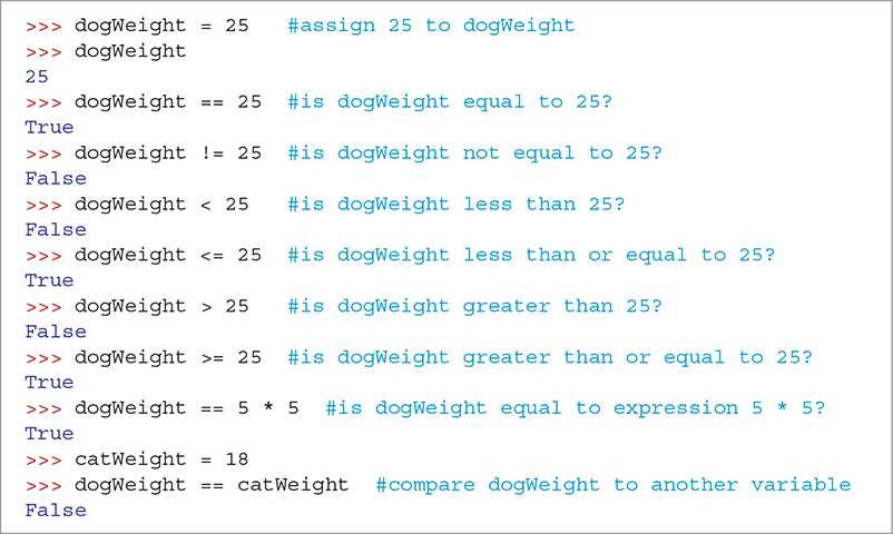
SESSION 2.9 Evaluating simple relational expressions
2.6.2 Compound Boolean Expressions and Logical Operators
In Python, compound Boolean expressions are composed of simple Boolean expressions that are connected by one of the logical operators and, or, and not. TABLE 2.4 defines the behavior of the Python logical operators. Note that any Python expression can be used as part of a Boolean expression. Most often the expressions will be relational expressions.
TABLE 2.4 Logical Operator Behavior |
|
|---|---|
| Expression | Evaluation |
x and y |
If x is False, return x; otherwise return y. |
x or y |
If x is False, return y ; otherwise return x. |
not x |
If x is False, return True; otherwise return False. |
It is important to understand that Python evaluates a Boolean expression exactly as indicated in Table 2.4. Python uses short-circuit evaluation of a Boolean expression, which means it evaluates only as much of the expression, from left to right, as necessary to determine whether the expression is True or False.
For example, in this Boolean expression using or,

Python needs to evaluate only the expression 3 < 7 because this is True and only one expression needs to be True for a compound expression with or to be True. It makes no difference to the outcome if 10 < 20 is True or False. Similarly, in this expression using and,

Python needs to evaluate only the 10 > 20 part of the expression, because 10 > 20 is False. Thus, the whole expression must be False, because with and both expressions need to be True for the whole expression to be True. As in the previous example, it makes no difference to the outcome whether 3 < 7 is True or False. SESSION 2.10 shows the logical operators in action.
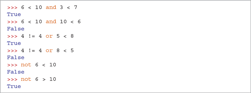
SESSION 2.10 Evaluating compound Boolean expressions
2.6.3 Selection Statements
Once we are able to ask a question by writing a Boolean expression, we can turn our attention to using that question for making a decision. In computer science, decisions are often called selection because we wish to select between possible outcomes based on the result of the question we have asked. For example, when we go outside in the morning, we might ask the question, “Is it raining?” If it is raining, we will grab an umbrella. Otherwise, we will pack our sunglasses. In this case, we are selecting which item to take with us based on the condition of the weather.
Until now, the statements in our Python programs have been executed in sequence—one at a time, in the order that they were written. We now introduce a new statement called a selection statement, also known as an if statement. The selection statement contains a question and other groups of statements that may or may not be executed, depending on the answer to the question. Most programming languages provide two versions of this useful statement: the if-else and the if.
The if-else statement looks like this:
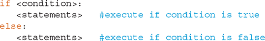
The keyword if is followed by a Boolean expression that is used as a condition for the selection. When the Boolean expression is evaluated, the result will either be True or False. On the one hand, if it is True, the first group of statements is executed in sequence and the second group is skipped. On the other hand, if the condition is False, the first group is skipped and the second group is executed in sequence (see FIGURE 2.11). In this way, it is possible to perform different actions based on the result of the question that was asked.
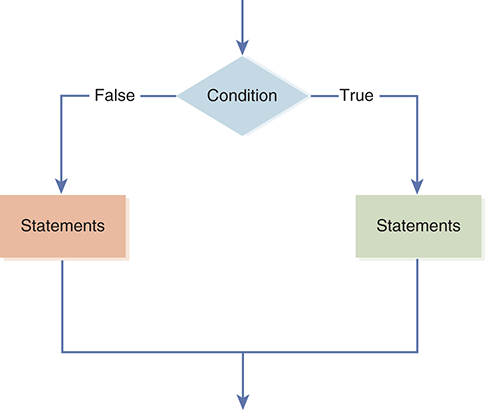
FIGURE 2.11 The logical flow of an if-else statement.
Notice that a colon follows the condition, and that each group of statements is indented just like a for loop or function definition.
For example, in SESSION 2.11, the variables a and b are assigned initial values. The if-else statement that follows asks the question of whether a is greater than b. Since a is greater than b, the first group of statements (in this case, only one) is executed, and the value of the variable c is set to 10. We can verify that this did occur by printing the variable c after the statement is done.
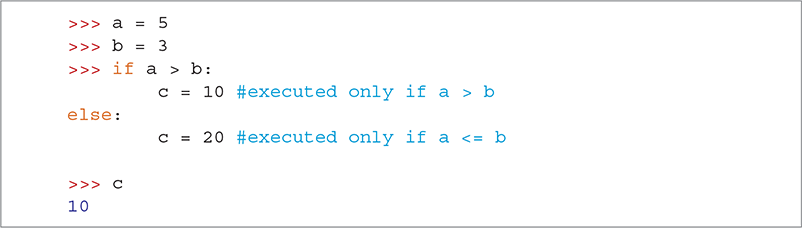
SESSION 2.11 Executing a simple if-else selection statement
The other variation of the if statement does not provide an else clause. It looks like the following:

As before, the condition is evaluated, and the result will be either True or False. If the result is True, the indented group of statements is executed in sequence. Conversely, if the condition is False, nothing is performed, the statement completes, and the program goes on to the next statement following the if statement (see FIGURE 2.12).
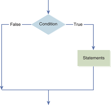
FIGURE 2.12 The logical flow of an if statement.
For example, in SESSION 2.12, the variables a and b are again assigned initial values. The if statement that follows asks the question of whether a is greater than b. Because the answer is True, the group of statements (again, only one statement in this case) is performed, and the value of the variable c is set to 10. In the second selection, however, the condition ( b > a ) evaluates to False, so the value of the variable c is not modified. In this case, the value of c remains the same as it was before the selection.
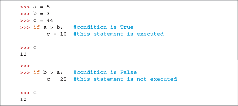
SESSION 2.12 Executing a simple if selection statement
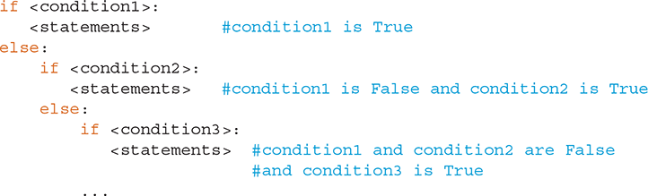
Since the statements contained within a selection statement can be any legal Python statement, it is certainly possible to place one if statement inside another. This practice is sometimes referred to as nested selection. The following if-else statement has two nested if-else statements:
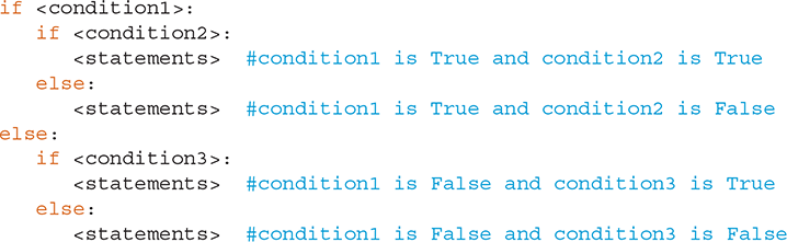
The result of this structure is to decide among four groups of statements. If condition1 is True, then the first nested if-else is performed. If the nested condition2 is also True, then its first group of statements is performed. However, if the nested condition2 is False, its second group of statements is executed. Likewise, if condition1 is False, the second nested if-else will be performed. In this way, we are able to decide among four groups of statements by using the results of three conditions.
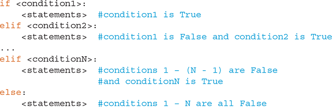
One common pattern for nested selection is called tail nesting. With tail nesting, all of the nested selection occurs in the else of the previous if-else statement. The structure looks like this:
This tail nesting pattern is so common that Python provides a shorter version known as the elif statement. In this statement, the combination of the else and the next if allows us to simply list the conditions and associated statements one at a time without additional indentation. Note that the last case uses a simple else.
2.6.4 Completing the Implementation
We are now ready to complete our Monte Carlo approximation of π. Again, we will use the abstraction idea to build a function that will return the approximate value of π. For this function, we will use the number of darts as the input parameter. The more darts we throw, the better our approximation should be.
Recall the basic steps of the simulation. First, pick a random point on the square board. Next, decide whether that point is also in the transcribed quarter-circle, keeping a count of those darts that hit within the circle. After all the random points have been tested, the approximate value of π will be four times the fraction of darts that land inside the circle.
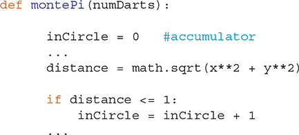
To keep a count of the number of points that fall in the circle, we will again use the accumulator pattern with a variable initialized to 0. Every time a point lands in the circle we will increment our accumulator variable by 1. Remember that the initialization needs to occur outside the iteration.
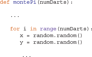
To process each point, we must first generate the two values that will make up the random location. To do so, we will use the random function from the random module. Because we will consider the first value to be the horizontal measure and the second to be the vertical measure, we will use x and y as their names.
We now need to decide whether the random point is inside the circle. For this, we can use the formula for finding the distance between a point and the origin (0, 0): ![]() . The
. The math module provides us with the sqrt function needed to calculate the square root.
Once we have the distance, we can use our selection statement to decide whether we want to count the point. Recall that if the point is within 1 unit of the center, it is in the circle and we should perform our increment step. A simple if statement will work nicely here.
Finally, as shown in LISTING 2.5, the calculation of pi is the ratio of the number of points that occur in the circle to the number of total points. That ratio must then be multiplied by 4 to get the approximation.
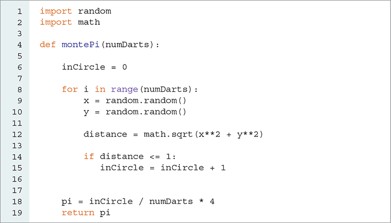
LISTING 2.5 A function to compute pi using the Monte Carlo simulation
SESSION 2.13 shows the function at work. Note that as we increase the number of points (darts) used in the simulation, the accuracy improves. Nevertheless, the results will vary from one execution to the next with the same number of darts because of the randomization of points.
SESSION 2.13 Using the montePi function
2.6.5 Adding Graphics
As a final variation on this simulation, we will use our turtle to provide a graphical animation of the algorithm. We can use the turtle to show the random points as they are being generated. In addition, depending on the location of the point, we can use color to show the location as either inside or outside the circle.
To begin using the turtle, we must import the turtle module. In our previous turtle examples, the turtle window was created automatically when we created a new turtle object. The turtle module also makes it possible to create the drawing window, or screen, separately, and then add the turtle later. By doing this, we can call methods to customize the drawing window.
The way we create a drawing window is to use the Screen constructor contained in the turtle module. The statement wn = turtle.Screen() will create a new drawing window and name it wn. This method and several other Screen methods of the turtle module are described in TABLE 2.5.
TABLE 2.5 Screen Methods in the Turtle Module |
|
|---|---|
| Function | Description |
Screen() |
Constructor that creates a TurtleScreen object to be used as a drawing window |
setworldcoordinates(xLL, yLL, xUR, yUR) |
Adjusts the window coordinates so that the point in the lower-left corner of the window is (xLL, yLL) and the point in the upper-right corner of the window is (xUR, yUR) |
exitonclick() |
Closes the window when the user clicks the mouse somewhere within the window |
Our next step is to set up the “dartboard” described earlier. Recall that the simulation works by generating numbers between 0 and 1 as locations for the random points. To show this, we can adjust the coordinate system used by the drawing turtle so that the area on which we will be drawing fills more of the screen. FIGURE 2.13 shows the original diagram for the simulation set inside the window.
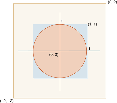
FIGURE 2.13 Setting the world coordinates for the graphical simulation
To modify the coordinate system of the drawing window, we will use a Screen method called setworldcoordinates. This method takes four pieces of information: (1) the x-coordinate of the lower-left corner, (2) the y-coordinate of the lower-left corner, (3) the x-coordinate of the upper-right corner, and (4) the y-coordinate of the upper-right corner. These two points will denote the coordinates of the lower-left and upper-right corners of the window used by the drawing turtle. Because we want the window to contain points from (–2, –2) at the lower-left corner to (2, 2) at the upper-right corner, we will call the setworldcoordinates method using these parameters:

We could have made this window any size we wish. However, the larger the window, the smaller the actual area of the simulation.
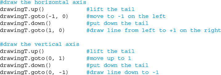
Now that the window is set up, we want to draw horizontal and vertical axes so that when we plot the points, it will be clear where they are being placed. Recall that the drawing turtle will draw a line whenever its tail is in the down position, but not when its tail is up. So all we need to do is:
Raise the tail.
Go to the starting position for an axis without drawing a line.
Lower the tail.
Go to the ending position for the axis to draw the line.
The Python code to accomplish this is shown here:
The remaining portion of the program simply asks the drawing turtle to place dots at the random points as they are generated. To do this, we can go to the location and then use the dot method to ask the turtle to create a dot at the current location.
The only additional feature that we will add is color to indicate whether the point is inside or outside the circle.
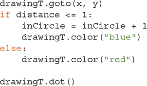
Since there are now two choices depending on the location of the point, it makes sense to use the if-else version of the selection statement described earlier. If the point is inside the circle, we change the tail color to blue and count the point. Otherwise, if the point is outside the circle, we change the tail color to red. In Python, this translates to the following sequence:
LISTING 2.6 shows the complete function, including the commands to use the turtle to show the simulation in progress. Note that the dot is drawn after the if statement executes. This needs to be done only once for each iteration. Also, because we do not want to draw lines when we move the turtle using the goto method, we lift the tail before beginning the for loop. The dot method will leave a mark even if the tail is up. FIGURE 2.14 shows what the simulation might look like. You can see how the quarter-circle is beginning to emerge. As more and more points are used, this would become even clearer.
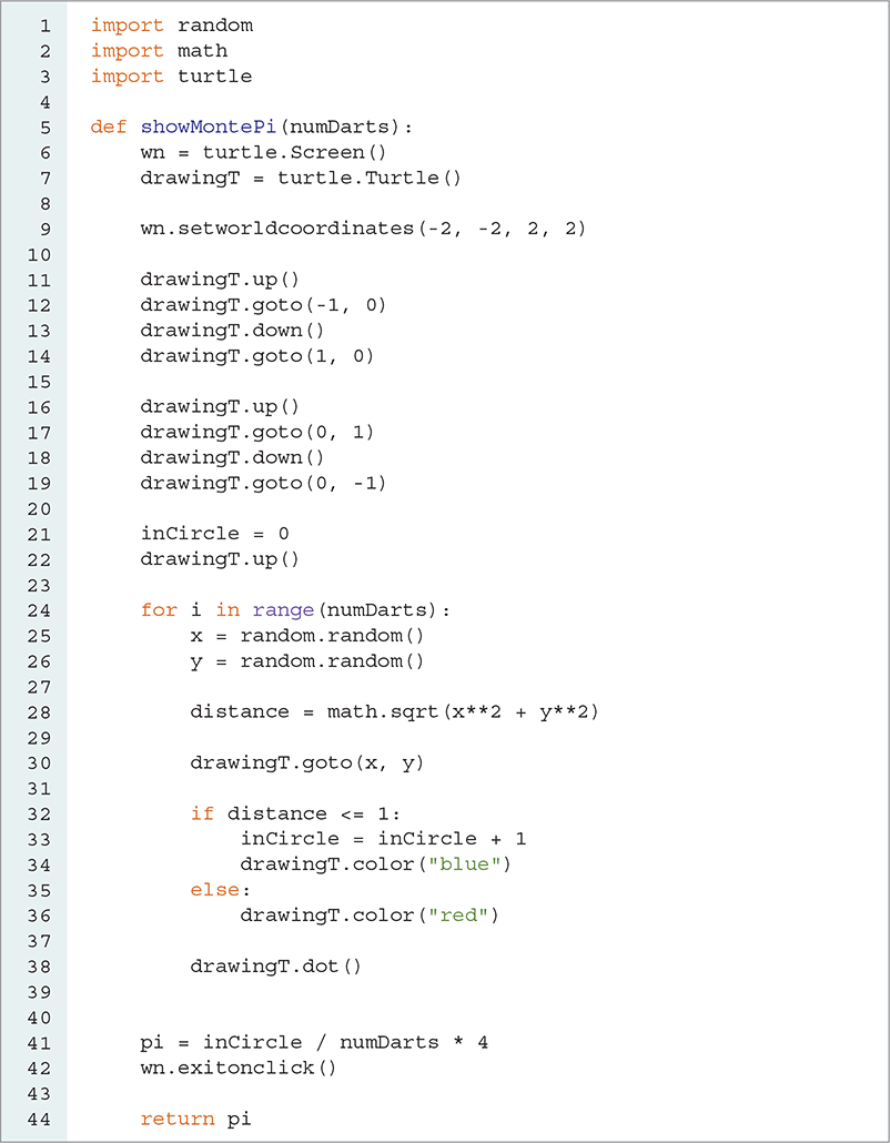
LISTING 2.6 Adding graphics to the Monte Carlo simulation
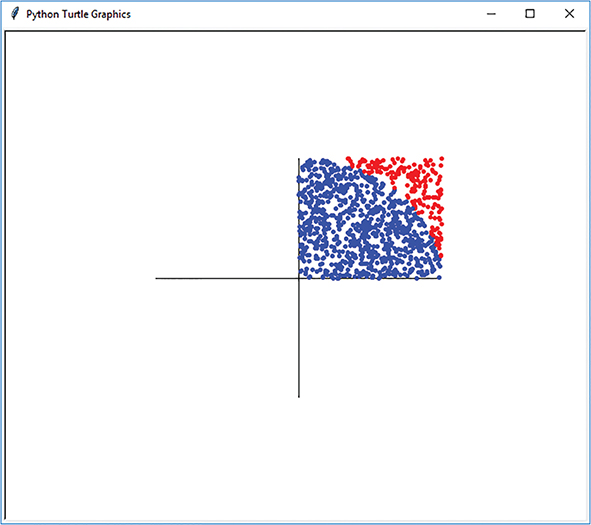
FIGURE 2.14 Visualizing the simulation with 1000 points.
At the end of the showMontePi function, we used one additional Screen method called exitonclick. This method tells the drawing window to “freeze” until the user clicks somewhere inside the window. If we don’t use this method, the turtle drawing window will automatically close when the program ends. We placed that call to exitonclick immediately before returning from the function.