2.5 Accumulator Approximations
The pi approximation techniques that follow will use mathematics based on infinite series and infinite product expansions. The basic idea is that by adding or multiplying an infinite number of arithmetic terms, we can get increasingly closer to the actual value we are trying to compute. Although the mathematics of these approaches is beyond the scope of this text, the patterns provide excellent examples of arithmetic processing.
2.5.1 The Accumulator Pattern
To use these techniques, we will need to introduce another important problem-solving pattern known as the accumulator pattern. Your ability to recognize this commonly occurring pattern and then implement it will be especially useful as you encounter new problems that need to be solved.
As an example, consider the simple problem of computing the sum of the first five integer numbers. Of course, this is quite easy because we can just evaluate the expression 1 + 2 + 3 + 4 + 5. But what if we wanted to sum the first 10 integers? Or perhaps the first 100? The size of the expression would become quite long. To deal with this challenge, we can develop a more general solution that uses iteration.
Examine the Python code shown in SESSION 2.5. As you can see, the variable acc starts with a value of 0, sometimes called the initialization. Recall that the statement

will cause the loop variable x to iterate over the values from 1 to 5. FIGURE 2.5 shows how this statement can be used to create the running sum. Every time we pass through the body of the for loop, the assignment statement acc = acc + x is performed. Because the right-hand side of the statement is evaluated first, the current value of acc is used in the addition. To complete the assignment statement, the name acc is updated to refer to this new sum. The final value of acc is then 15.
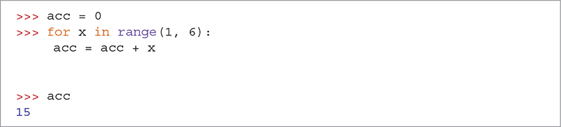
SESSION 2.5 Computing a running sum with iteration and an accumulator variable
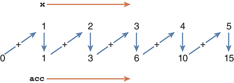
FIGURE 2.5 Using the accumulator pattern.
It might seem strange to see the same name appearing on both the left-hand and right-hand sides of the assignment statement. However, if you remember the sequence of events for an assignment statement you will not be confused:
Evaluate the right-hand side.
Let the variable on the left-hand side refer to the resulting object.
The variable acc is often referred to as the accumulator variable because it is continuously updated with the current value of the running sum. Now, whether we want the sum of the first five integers or the first 5000, the task is the same: Simply change the upper bound on the range and allow the accumulator pattern to do its work.
2.5.2 Summation of Terms: The Leibniz Formula
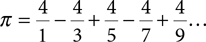
We can now turn our attention back to computing approximations of pi. As we suggested earlier, a number of formulas use the idea of infinite expansion. One of these is the Leibniz formula, named after Gottfried Leibniz, a German mathematician and philosopher who lived from the mid-1600s to the early 1700s:
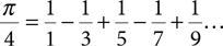
A bit of algebra—namely, multiplying every fraction by 4—will give us a much easier form:
To successfully turn this formula into Python code, we must look for the following patterns:
▶ All the numerators are 4.
▶ The denominators are odd numbers in increasing sequence starting at 1.
▶ The sequence of fractions alternates between addition and subtraction.
We will deal with each of these patterns shortly.
The accuracy of the approximation will depend on the number of terms we use; that is, more terms will lead to a better approximation. With this point in mind, we can think about the abstraction pattern and construct a function that will take the number of terms as a parameter and return the value of pi that those terms produce (see FIGURE 2.6).
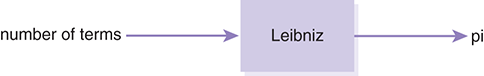
FIGURE 2.6 Abstraction for the Leibniz formula.
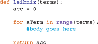
Because the right-hand side of this formula is a sum of terms, we are inclined to think about the accumulator pattern. To set up this pattern, we will need an accumulator variable and an iteration. In this case, the number of terms will be a parameter to the function, so we can start with the following structure:
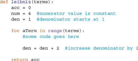
Because each term is a fraction, we need to build both the numerator and the denominator. Each fraction will have the same numerator, 4. The denominator in each case will change, starting at 1 and increasing by 2 each time. We can achieve this effect by using the accumulator pattern. We will start the accumulator variable den at 1, and the statement den = den + 2 will cause an accumulation each time through the iteration.
We now need to determine how to compute each fraction term. To start, we can divide the numerator by the denominator. However, we still need to alternate the terms between positive and negative. An interesting way to do this is to take advantage of the loop variable aTerm.
FIGURE 2.7 shows the first five fractions of the sequence and how each term is related to the value of the loop variable aTerm. Notice that when aTerm is 0 or an even number, the term is positive; when aTerm is 1 or an odd number, the term is negative.
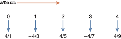
FIGURE 2.7 The fractions of the Leibniz formula.
One way to produce this pattern is to raise −1 to the power of aTerm. This will create a sequence that alternates between 1 and −1; we multiply each fraction by the current number in the sequence. Each time through the iteration, nextTerm is computed by dividing the numerator by the denominator and multiplying the result by a power of −1. The result can then be added to the accumulator variable, acc, as shown in LISTING 2.3. Then we get ready for the next term by adding 2 to the denominator accumulator. Notice that we have two accumulator variables in this function, acc and den. SESSION 2.6 shows the function in action. Once again, note that increasing the number of terms gives a better approximation of pi.

LISTING 2.3 A function to compute pi using the Leibniz formula
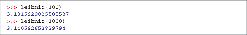
SESSION 2.6 Using the leibniz function
2.5.3 Product of Terms: The Wallis Formula
Our second example of the accumulator pattern will use an infinite product instead of an infinite sum. Shown here is the Wallis formula, named after the British mathematician John Wallis, a contemporary of Leibniz:
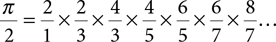
Like the infinite sum formula, this formula requires that we decide how many terms we want to use. In this case, you can see that the right-hand side makes use of the multiplication operator. One thing to recognize right away is the impact that this multiplication will have on the initialization of the accumulator variable. If we use 0 as before, we will always get a result of 0. For this reason, in this case, we will want to initialize the accumulator variable to 1.
The next pattern we should consider is the fractions themselves. At first glance, it might seem as if they are unrelated. However, if you look at them in pairs (see FIGURE 2.8), you can see that each pair of fractions shares a common numerator, starting with 2 in the first pair and increasing by 2 for each subsequent pair.
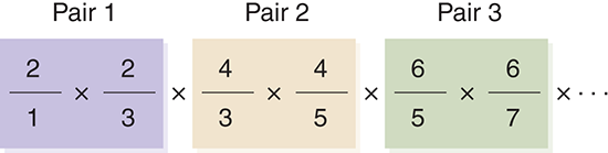
FIGURE 2.8 Fraction pairs in the Wallis formula.
Using abstraction once again, we can now begin to construct a function that will accept the number of pairs as the input parameter and return the value of pi produced by the infinite product. We can initialize our numerator to 2.
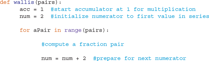
Our next step is to calculate the actual fractions. We have already noted that they come in pairs, so we need to look for the relationship between the numerator and the denominator within each pair. For each numerator, the denominators are one less and one more. In other words, if the numerator is n, the left fraction of the pair has a denominator of n − 1 and the right fraction of the pair has a denominator of n + 1. We can now calculate the two fractions and perform the accumulating multiplication.
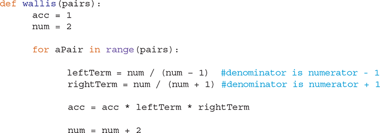
A final step: In the original Wallis formula, the value of the infinite product is equal to

This means that we must multiply the resulting product by 2 to get the approximation of pi that will be returned by the function. LISTING 2.4 shows the complete function. Note that the multiplication statement before the return is at the same indentation level as the return, rather than being inside the for loop. We want that multiplication to be done only once. SESSION 2.7 shows the result of invoking the function on different numbers of pairs.
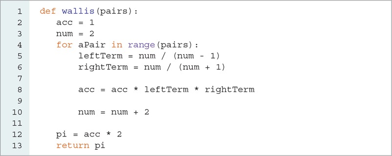
LISTING 2.4 A function to compute pi using the Wallis formula
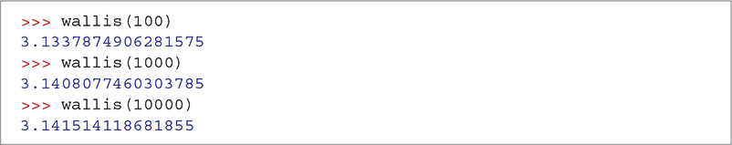
SESSION 2.7 Using the wallis function