7.4 Implementing Cluster Analysis on Simple Data
We now turn our attention to the fundamental steps of the cluster analysis technique. To concentrate on the algorithm, we use a very simple data set. Later, we will apply these same ideas to more complex data. Our example data in this section consists of exam scores for a group of 21 students taking an Introduction to Computer Science course. These scores represent the percentage of correct answers. The range of scores is between 0 and 100.
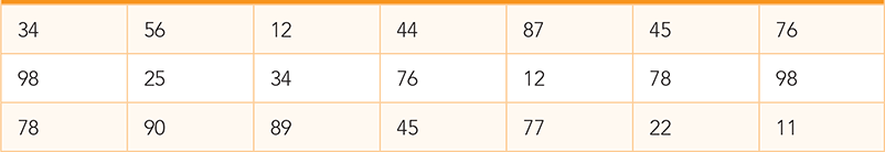
TABLE 7.1 provides a simple listing of the scores. Our initial observation does not reveal any patterns. We could certainly use our previous work to compute descriptive statistics that might yield a bit more information, but in this case we are interested in identifying any patterns of similarity among the student scores. Cluster analysis could help us answer that question.
TABLE 7.1 Exam Scores for 21 Students |
|---|
|
7.4.1 Distance Between Two Points
One of the most important steps in the cluster analysis algorithm is to classify data points according to their similarity to other data points. To measure this similarity, we need some way to determine whether two points are “close” to each other. This can be done by computing a value that we will call the “distance” between two data points.
We can measure the distance between two data points in many different ways. For our purposes, we use a simple measure known as the Euclidean distance. Consider the two data points A and B, shown in FIGURE 7.3. If we assume that point A has location X1 and point B has location X2, then the distance between them, d, will be the simple difference between the two location values: d = X2 − X1. Because we do not know whether this difference will be positive or negative, however, we should use the absolute value.
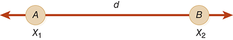
FIGURE 7.3 Simple distance between two points.
An alternative way to eliminate negative values is to square them, as the squaring operation will always result in a positive number. To get the original positive value, we can then take the square root. Using this approach yields the equation
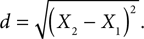
Although this may seem like extra work, the benefit can be seen if we extend our example to computing the distance between two points in more than one dimension. FIGURE 7.4 shows our two points. This time the location of point A is given by the pair (X1, Y1). Likewise, point B has location (X2, Y2). To compute the distance d between the two points now requires that we use the two-dimensional version of the previous equation, which is also known as the Pythagorean theorem:
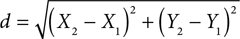
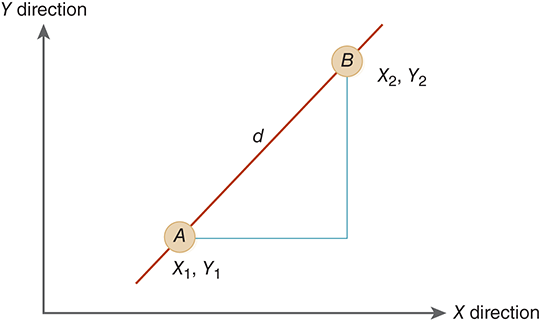
FIGURE 7.4 Two-dimensional distance between two points.
In general, this calculation can be extended to handle any number of dimensions. The distance between two data points in n dimensions can be computed as the square root of the squares of the differences between each of the n coordinates. For example, consider a point A in five-dimensional space with location (23, 44, 12, 76, 34). If point B has location (67, 55, 85, 23, 24), the distance between point A and point B is given by

LISTING 7.1 shows a function to compute the distance between two points. Each point is defined as a list of n coordinate values. Starting with sum initialized to 0, we iterate through the coordinate list. If we assume that each point has the same dimensionality, the index range for point1 will be the same as the index range for point2. Line 4 computes the square of the difference, and line 5 adds that value to the running total. Finally, the square root is computed and returned. The euclidD function assumes that the math module has been imported.
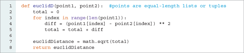
LISTING 7.1 Computing the Euclidean distance between two points
7.4.2 Clusters and Centroids
Clusters of data points exhibit the characteristic that all the points in the cluster are similar to one another. Another way to think about this similarity is to suggest that all the data points in the cluster are associated with some notion of a center point. This center point can be used to identify a particular cluster.
A centroid is defined as the mean of a collection of data points. Each cluster will have a centroid that represents the center of the cluster. Note that the centroid does not need to be an actual point in the cluster: It is simply the “point” that tends to be in the center of all others.
To compute the centroid for a set of points, we calculate the mean value for each dimension. For example, if we have two points in two dimensions, (3, 7) and (1, 5), the centroid will be
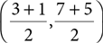
or (2, 6). This pattern can be extended to include any number of points with any number of dimensions.
FIGURE 7.5 shows three points with two dimensions: (2, 4), (5, 8), (8, 6). The centroid (5, 6), shown by the star, represents the notion of the center with respect to the three points. If these points were considered to be a cluster, we could use the centroid as its identity.
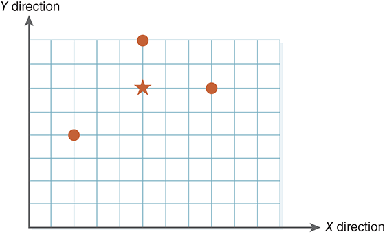
FIGURE 7.5 The centroid of three points in two dimensions.
7.4.3 The K-Means Cluster Analysis Algorithm
Many clustering algorithms have been developed. Here, we present one of the oldest and easiest-to-understand techniques—the K-means algorithm. The basic steps of this algorithm, which is simple to both describe and implement, are as follows:
Decide how many clusters you would like to create; call that number
k.Randomly choose
kof the data points to serve as the initial centroids for thekclusters.Repeat the following steps for a specified number of times or until the clusters are stable:
Assign each data point to a cluster corresponding to its closest centroid.
Recompute the centroids for each of the
kclusters.
Show the clusters.
The number of iterations performed in Step 3 can vary. Sometimes, a simple maximum iteration value is used. Alternatively, the step can be repeated until the clusters become stable. Clusters are considered to be stable when the centroids no longer change from iteration to iteration. Under some circumstances, this state may never occur, as the points will tend to oscillate back and forth between different clusters.
Choosing the initial centroids randomly, however, can lead to empty clusters and results that differ from run to run. We will mention more of the shortcomings of this approach in Section 7.6.
7.4.4 Implementation of K-Means
We now implement the cluster analysis algorithm on the exam data set. We assume that the data is stored in a file named cs150exams.txt, with one score per line. There is no order or additional identifying information in the data file. We need to process the file line-by-line and extract the exam scores.
Since we need to keep the individual scores separate, we assign an identification key to each score; the keys start with 1 and continue through n, where n is the number of scores. In other words, we identify each score using the line number from the file. We can then associate the key with any additional information that may be present in the data file. (This will be useful in later examples.)
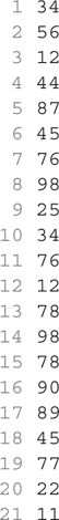
The cs150exams.txt file (with line numbers indicated in gray) is shown below. The line numbers are not part of the file.
LISTING 7.2 shows a function that takes a filename as a parameter and returns the dictionary as described earlier. We first open the file, next create an empty dictionary, and then start accessing each line of the file. Since the only data on the line is the test score, we can simply use the int function to convert the test score to an integer. Line 10 enters the score in the dictionary associated with the key. Note that the score is placed in a list before it is added to the dictionary. Recall that each data point can be multidimensional. Even though these scores are not multidimensional, the euclidD function will expect the data points to be lists of values.
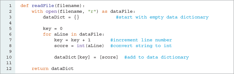
LISTING 7.2 Processing the exam score data file
SESSION 7.1 shows the data dictionary created by executing the readFile function with the cs150exams.txt file.
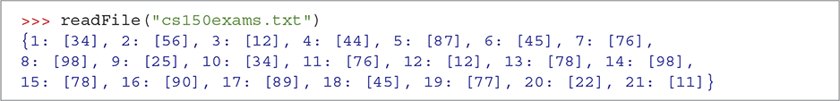
SESSION 7.1 The data dictionary created by the readFile function
The next step is to choose k, the number of clusters. Often the number of clusters may be based on some preconceived notion about the data values. In this case, we create five clusters, assuming that one possible reason for clustering the data is to look for groupings that represent the five grading categories—say, A, B, C, D, or F.
Now we need to pick k random data values to be our initial centroids. To implement this step, we use the randint function from the random module. This random number generator will pick an integer in the range [a, b] including the endpoints. For example, randint(2, 5) will return a random integer between 2 and 5 inclusive.
It is important to choose unique centroid values. If we were to simply iterate through the data k times, there is no guarantee that the k values will not contain a duplicate. To satisfy this requirement, we use a while loop.
Indefinite Iteration
Most of the iterations we have performed up to this point have used a for loop. Recall that the for loop allows us to repeat a group of statements, once for each value in a sequence. For example, in the Python statement
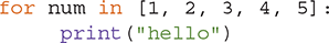
the print function, which makes up the body, will be executed (repeated) five times. Each time through the loop, the loop variable num will take on a subsequent value from the list. The total number of iterations is strictly determined by the number of items in the sequence provided.
This type of iteration is referred to as definite iteration because the number of repetitions is (definitely) known based on the size of the iteration sequence. Whenever we know the number of times we want to iterate, the for loop is the appropriate construct to use.
In other cases, we do not know exactly how many iterations will be necessary. That is, we know that we want to repeat a process, and we know that we want to eventually stop the repetition, but we are not certain about the actual number of repetitions to be performed. In such cases, we need a form of iteration known as indefinite iteration, in which we state a condition that will be used to decide whether to continue iterating. If the condition is satisfied, we will perform the loop again and then recheck the condition. When the condition no longer holds, the loop will no longer be repeated.
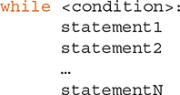
The while Loop
To implement indefinite iteration in Python, we use the while loop, which we introduced in Chapter 5. This construct is similar to the for loop and the if statement in that it controls a body of statements. As with other structured statements, the statements in the body are indented.
As a review, FIGURE 7.6 shows the logical flow of control created by the while loop. The controlling condition can be any Boolean expression—that is, any expression that evaluates to True or False. The statements in the body will be executed repeatedly until the condition evaluates to False. If the Boolean expression is False initially, the statements will never be executed. In other words, the statements in the body will be executed zero or more times, depending on the value of the condition.
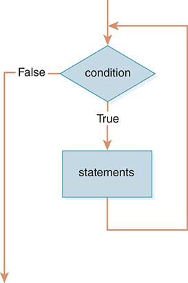
FIGURE 7.6 The while loop.
As an example, consider the familiar code fragment shown in LISTING 7.3. Here we are using a for loop to compute the sum of the first 10 integers. Line 1 initializes an accumulator variable, total, that is used to keep the running sum. The for loop header (lines 2) automatically iterates through the sequence produced by the range function, [1, 2, 3, 4, 5, 6, 7, 8, 9, 10], assigning each subsequent value to the loop variable aNum. The body of the iteration (line 3) adds the value of aNum to the accumulator. When the loop ends, the value of total is printed.
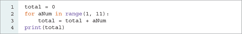
LISTING 7.3 Summation from 1 to 10 using a for loop
We can rewrite this summation fragment using a while loop, as shown in LISTING 7.4. The algorithm remains the same—that is, we iterate over the values from 1 to 10 and add each to an accumulator variable called total. As before, line 1 initializes the accumulator variable, and line 4 performs the addition to compute the running sum. Lines 2, 3, and 5 taken together form the iteration, or loop, control.
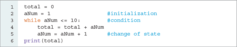
LISTING 7.4 Summation from 1 to 10 using a while loop
Note that the iteration process is not simply the while <condition>: but also includes a number of other statements. To write a correct iterative process using a while loop, you must include three parts: the initialization, the condition, and the change of state. All of these parts must work together for the iteration to succeed.
Line 3 of Listing 7.4 provides the condition upon which the iteration will continue. In this example, as long as the value of the variable aNum is less than or equal to 10, the body statements will be executed. Recall that the while loop evaluates the condition first, before performing the body of the loop. Any variables used in the condition must have their initial values set prior to entering the while loop. Since the goal of this iteration is to count from 1 to 10, it makes sense to initialize the value of aNum to 1.
If the condition succeeds, control proceeds to the body. After the body is executed, the condition is rechecked. The only way for the iteration to stop is for the condition to fail, which requires some change to occur inside the body that will directly impact the result of the condition. This change of state is a critical part of the iteration. Without it, the condition that was True originally would remain True forever and the while loop would never stop. In Listing 7.4, line 5 provides this change of state. Each time through the body, the value of aNum is incremented by 1. Eventually, the value of aNum will reach 11, which will cause the condition to fail.
Beginning programmers often forget one of the three parts of the while loop or include all three parts but with inconsistencies. As an example, consider LISTING 7.5. Here, the initialization and the condition are correct, but the change of state is missing—that is, the value of aNum never changes. Thus, once the condition is found to be True, nothing in the loop body will change the condition to False. The result will be a while loop that never stops—an infinite loop.
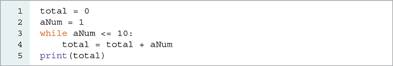
LISTING 7.5 Infinite loop
LISTING 7.6 shows a function that will process the data file using an indefinite iteration. Line 7 uses the readline method to get the next line of the file. This method will return the empty string, "", when there are no more lines in the file. The condition will check for the empty string and allow execution of the body only if a line of data was read.
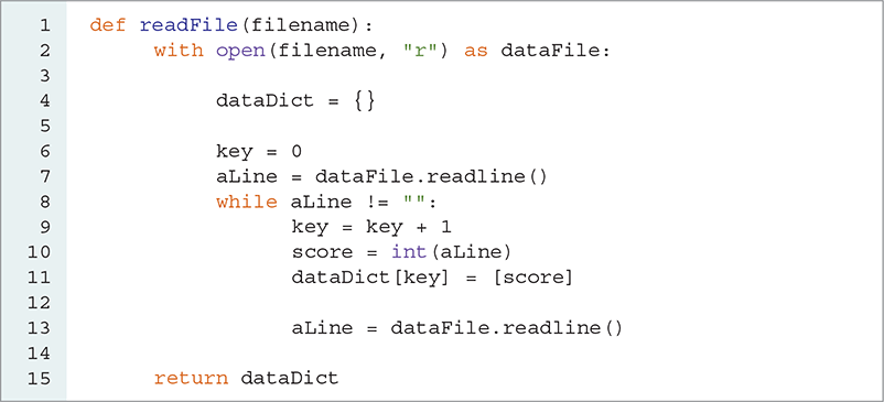
LISTING 7.6 Processing the exam score data file using indefinite iteration
After the line has been processed, the condition must be rechecked. Before this can happen, a change of state must occur. For this example, the change of state is to read the next line of data from the file. Either a valid line or the empty string will be returned, and the condition can be reevaluated.
If you run this function, you will see that the same data dictionary will be created as the previous version of readFile using a for loop.
7.4.5 Implementation of K-Means, Continued
The function shown in LISTING 7.7 implements the centroid selection process. It takes the number of centroids (called k) and the data dictionary as parameters. Line 2 creates an empty list of centroids. Our task is to fill this list with k randomly selected data points. As we do not want to use a key twice, we will store a list of the selected keys and check each randomly selected key against this list. If the key is already in the list, we will not include its data point as a centroid, but instead will pick another key randomly. This process will continue until k centroids have been selected. Because we do not know how many random selections will be required, we will use a while loop. This function assumes that the random module has been imported.
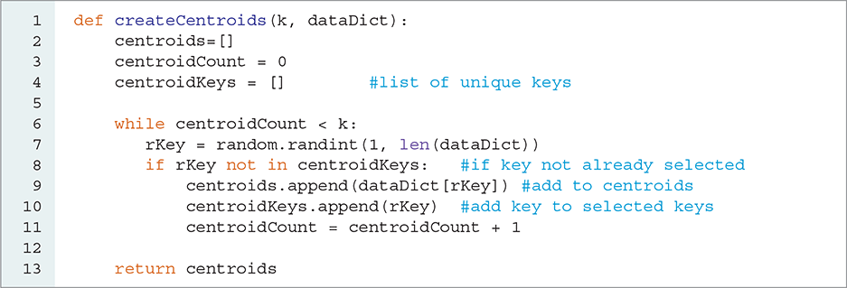
LISTING 7.7 Choosing k random centroids
We keep track of the number of valid centroids that have been found with centroidCount. As long as that number is less than k, we continue to generate random keys. If an unused key is found, it is added to the lists and the count is incremented (line 11).
LISTING 7.8 implements a function to create the clusters. The createClusters function takes as parameters the number of clusters (again called k), the previously created centroids, the data dictionary, and the number of repetitions, and it returns a list of the clusters. Each cluster is represented by a list. As we have a collection of clusters, a list of those cluster lists will be the appropriate way to store them. Lines 4–6 create this list of k empty clusters.
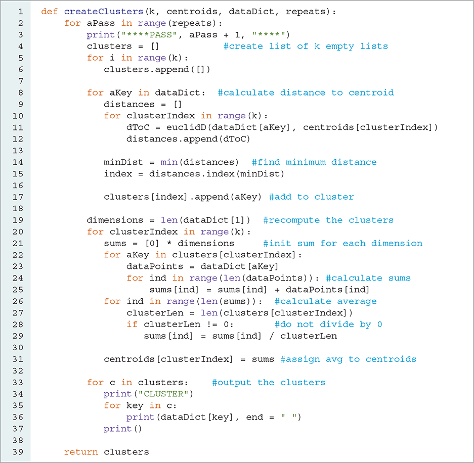
LISTING 7.8 Creating the clusters
We then go through each item in our data dictionary and assign it to the proper cluster. Recall that we have a list of centroids, one for each cluster. We want to assign each data point to the cluster with the closest centroid. We can do this by using our distance function, euclidD, described earlier.
As there are k clusters, each data point will have k distances associated with it, one from each centroid. Line 9 creates an empty list of distances, and lines 10–12 compute the distance between the data point and each centroid. These distances are placed in the distances list. The distances, centroids, and clusters lists are parallel to one another. In other words, for any particular index number i, i refers to data for the same cluster in each list. FIGURE 7.7 shows the three parallel lists and the relationships among them.
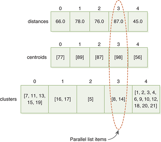
FIGURE 7.7 Parallel lists.
Once we have computed all of the distances, we can look for the closest centroid. Recall that Python provides a function called min that returns the smallest value in a list (line 14). Once we know the smallest value, we can use the list method called index to find where the minimum occurred in the distances list (line 15). The index of the minimum tells us the cluster to which the data point should belong. By using that index, we can access the list of clusters and append the key to the proper cluster (line 17). Again, it is important to remember that we are storing the keys instead of the actual data points.
The final step in the K-means algorithm requires that we recompute the centroids for each cluster. Since the centroid of a cluster is simply the average of all data points in the cluster, we can iterate through the points, create a running sum, and then divide by the number of points.
Lines 19–31 of Listing 7.8 implement the centroid recalculation. Line 19 is important because our data points can be multidimensional. In this line, dimensions is the number of dimensions within the data point. For our exam score example, its value will be 1. Recall that to compute the new centroid, we must take the average of the coordinate value in each dimension.
A list of running sums, represented by sums, will include a sum for each dimension of the data point. Each sum component is initialized to 0. Lines 24–25 calculate the running sums of the components, and lines 26–29 compute the average. The last statement (line 31) assigns the average to the proper position in the centroids list.
Recall that the clustering process is repeated a number of times. In Listing 7.8, the parameter repeats allows the user to decide how many iterations to perform. Listing 7.8 also includes a small fragment of code (lines 33–37) that prints out the contents of the clusters after each pass.
Finally, LISTING 7.9 shows a function that will perform the cluster analysis of the cs150exams.txt data file. It makes three passes through the data and produces five clusters.
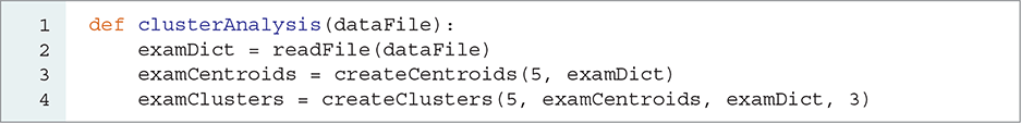
LISTING 7.9 Cluster analysis for the exam data set
When we run the program, it produces the output in SESSION 7.2. In the first pass, the exam scores are spread over the five clusters. The second pass shows that some of the scores have moved due to the new centroid values that were computed after the first pass. Finally, the last pass shows a final modification of the clusters. If we were using this analysis to assign grades, we might suggest that the first cluster would be the “A”s, the second cluster would be the “F”s, and so on. Of course, running the program again could give different results due to the random selection of initial centroids.
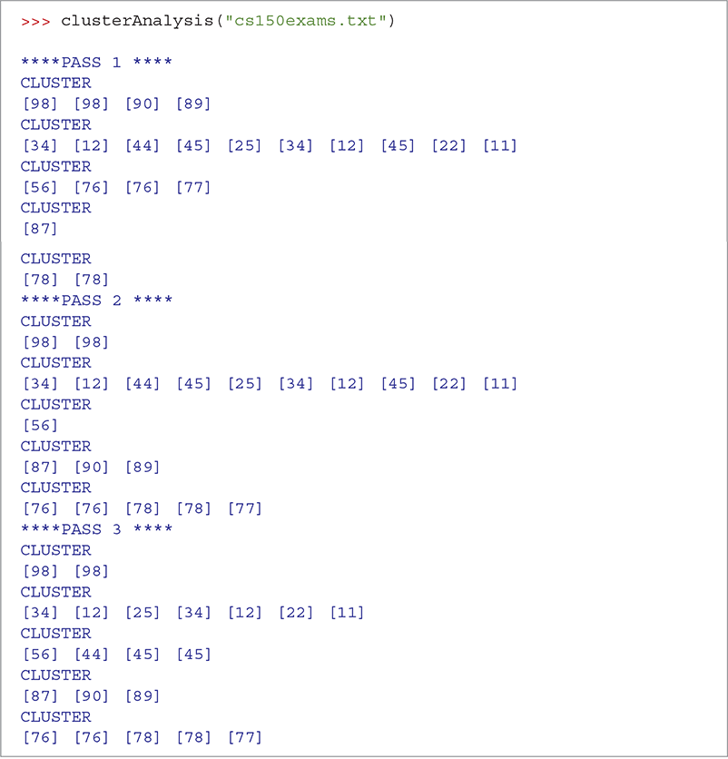
SESSION 7.2 Clusters of exam scores