6.5 Advanced Image Processing
We now turn our attention to some image processing algorithms that require the manipulation of more than one pixel either in the original image or in the new image. These techniques will require us to look for additional patterns in the way we process the pixels of the image.
6.5.1 Resizing
One of the manipulations most commonly performed on images is resizing—the process of increasing or decreasing the dimensions (width and height) of an image. In this section, we focus on enlarging an image. In particular, we consider the process of creating a new image that is twice the size of the original.
FIGURE 6.14 shows the basic idea. The original image is 3 pixels wide by 4 pixels high. When we enlarge the image by a factor of 2, the new image will be 6 pixels wide by 8 pixels high. This presents a problem with respect to the individual pixels within the image.
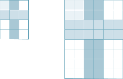
FIGURE 6.14 Enlarging an image by a factor of 2.
The original image has 12 pixels. No matter what we do, we will not be able to create any new detail in the image. In other words, if we increase the number of pixels to 48 in the new image, 36 of the pixels must use information that is already present in the original. Our problem is to decide systematically how to “spread” the original detail over the pixels of the new image.
FIGURE 6.15 shows one possible solution to this problem. Each pixel of the original will be mapped into 4 pixels in the new image. Every 1-by-1 block of pixels in the original image is mapped into a 2-by-2 block in the new image. This results in a 1-to-4 mapping that will be carried out for all the original pixels. Our task is to discover a pattern for mapping a pixel from the original image onto the new image.
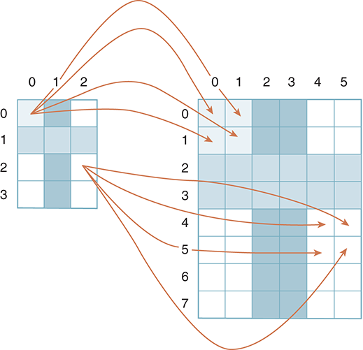
FIGURE 6.15 Mapping each old pixel to four new pixels.
An example of this mapping process shows that pixel (0, 0) will be mapped to pixels (0, 0), (1, 0), (0, 1), (1, 1). Likewise, pixel (2, 2) maps to pixels (4, 4), (5, 4), (4, 5), (5, 5). Extending this pattern to the general case of a pixel with location (col, row) gives the four pixels (2 × col, 2 × row), (2 × col+1, 2 × row), (2 × col, 2 × row+1), (2 × col+1, 2 × row+1). FIGURE 6.16 illustrates the mapping equations for a particular pixel. You should check your understanding by considering other pixels in the original image.
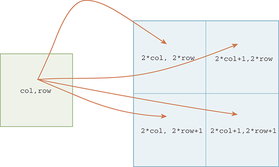
FIGURE 6.16 Mapping for a pixel at location (col, row).
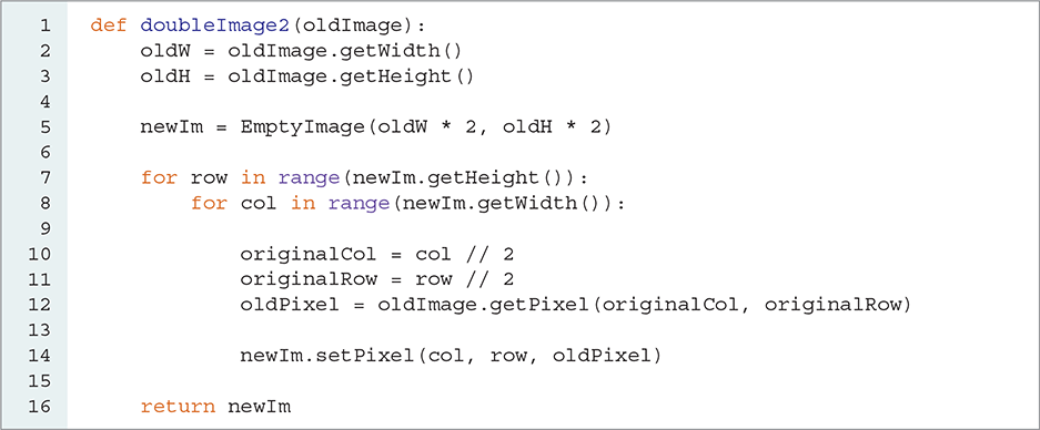
LISTING 6.8 shows the complete function for doubling the size of an image. Since the new image will be twice the size of the old image, it will be necessary to create an empty image with dimensions that are double those of the original (see lines 2–5).
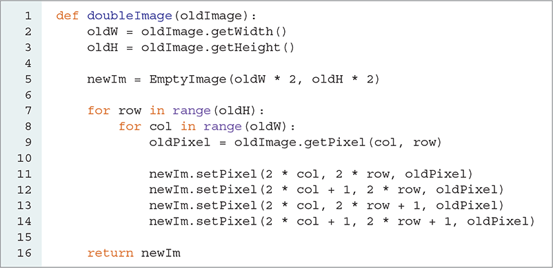
LISTING 6.8 Doubling the size of an image
Now we can use nested iteration to process each original pixel. As before, we use two for loops—one for the columns and one for the rows—to systematically process each pixel. Using the color components from each old pixel, we copy them to the new image. Lines 11–14 use the pattern discussed previously to assign each pixel in the new image. Note that each of the four pixels receives the same color tuple. In LISTING 6.9, we call the doubleImage function and place the newly sized image below the original image. FIGURE 6.17 shows the result.
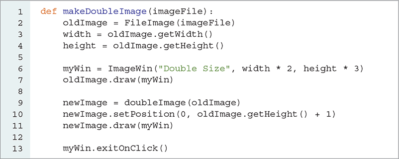
LISTING 6.9 Calling the doubleImage function
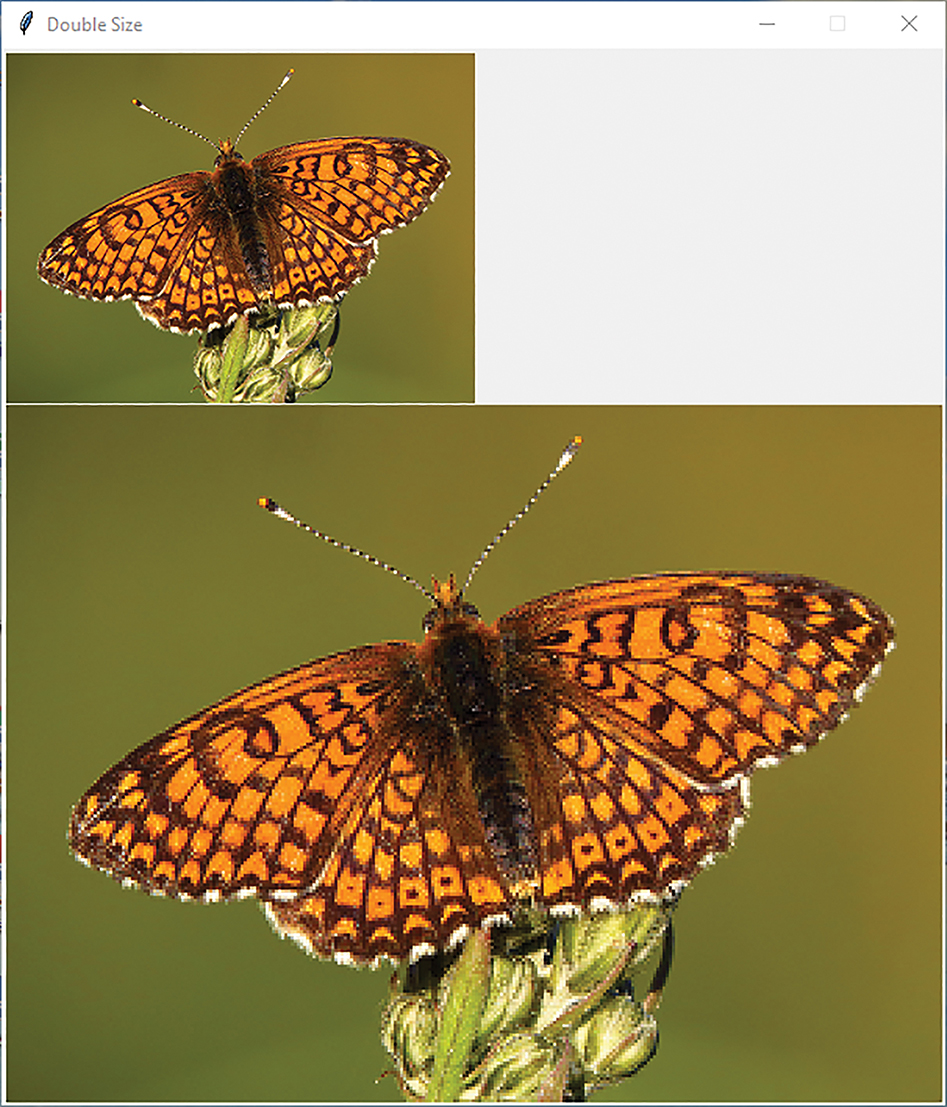
FIGURE 6.17 Enlarged image.
© 2001–2019 Python Software Foundation. All Rights Reserved. Images A and B © Luka Hercigonja/Shutterstock.
6.5.2 Stretching: A Different Perspective
The algorithm we just developed for enlarging an image requires us to map each pixel in the original image to 4 pixels in the new image. In this section, we consider an alternative solution: constructing a larger image by mapping pixels from the new image to the original image. Viewing problems from many different perspectives can often provide valuable insight. Our alternative solution takes advantage of this insight and leads to a simpler solution.
FIGURE 6.18 shows the same image, but with the pixel mapping drawn in the reverse direction. More specifically, instead of looking at the problem from the perspective of the original image, we now turn our focus to the pixels of the new image. As we process the pixels of the new image, we need to figure out which pixel in the original image should be used.
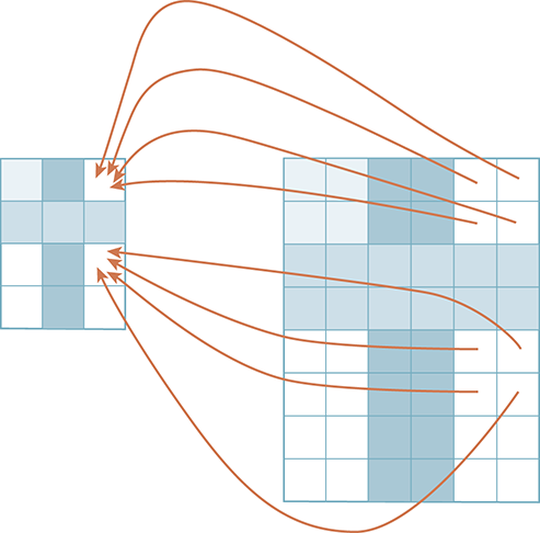
FIGURE 6.18 Mapping each of four new pixels back to one old pixel.
LISTING 6.10 shows the completed code for our new function, which will take an original image as a parameter and return the new, enlarged image. Again, we will need a new empty image that is twice the size of the original image. This time, we write our iteration to process each pixel in the new image. The nested iteration idea will still work, but the bounds will need to be defined in terms of the new image, as can be seen in lines 7–8.
LISTING 6.10 Doubling the size of an image: mapping new back to old
We now need to perform the pixel mapping. As we saw in the last section, the pixels at locations (4, 4), (5, 4), (4, 5), (5, 5) will all map back to pixel (2, 2) in the original. As another example (see Figure 6.18), pixels (4, 0), (5, 0), (4, 1), (5, 1) will all map back to pixel (2, 0). Our task is to find the mapping pattern that will allow us to locate the appropriate pixel in the general case.
Once again, it may appear that we have four cases because four pixels in the new image are associated with a single pixel in the original. However, upon further examination, we realize that is not true. Because we are considering the problem from the perspective of the new image, there is only one pixel that is of interest in the original. This suggests that we can use a single operation to map each of the new pixels back to the original. Looking at the example pixels, we can see that integer division will perform the operation that we need (see FIGURE 6.19).
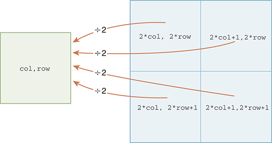
FIGURE 6.19 Mapping back using integer division.
In our example, we need an operation that can be done to both 4 and 5 and that will result in 2. Also, the same operation on 0 and 1 will need to yield 0. Recall that both 4//2 and 5//2 give a result of 2 because the // operator when working on integers gives an integer result, discarding the remainder. Likewise, 0//2 and 1//2 both give 0 as their result.
We can now use this operation to complete the function. Lines 10–11 extract the correct pixel from the original image by using the integer division operator to compute the corresponding column and row. Once the pixel has been chosen, we can assign it to the location in the new image. Of course, the result is the same as that seen in Figure 6.17.
As we stated earlier, enlarging an image provides no new detail. In some cases, the new image may look “grainy” or “blocky” because we are mapping one pixel to many locations in the new image. Although we cannot create any new detail to add to the image, it is possible to “smooth” out some of the hard edges by processing each pixel with respect to those around it.
6.5.3 Flipping an Image
We now consider manipulations that physically transform an image by moving pixels to new locations. In particular, we consider a process known as flipping. Creating a flip image requires that we decide where the flip will occur. We will assume that flipping happens with respect to a line called the flip axis. The basic idea is to place pixels that appear on one side of the flip axis in a new location on the opposite side of that axis, keeping the distance from the axis the same.
As an example, consider the simple image with 16 pixels in FIGURE 6.20 and a flip axis placed vertically at the center of the image. Because we are flipping on the vertical axis, each row will maintain its position relative to every other row. However, within each row, the pixels will move to the opposite side of the axis, as shown by the arrows. The first pixel will be last, and the last pixel will be first.
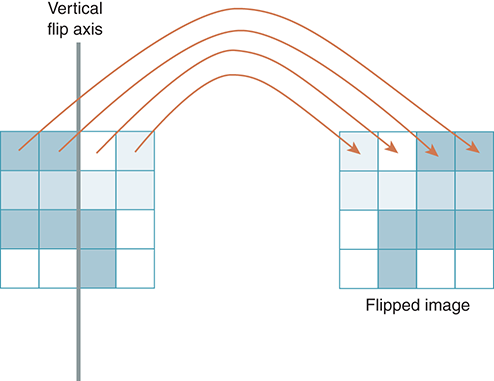
FIGURE 6.20 Flipping an image on the vertical axis.
The structure of this function is similar to that of the other functions we have written thus far. We build our nested iteration such that the outer iteration will process the rows and the inner iteration will process each pixel within the row. LISTING 6.11 shows the completed function. Because we are flipping the image rather than resizing it, the new image will have the same height and width as the original image.
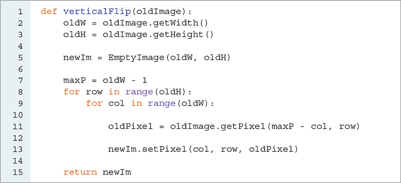
LISTING 6.11 Creating the vertical flip of an image
We need to discover a pattern to map each pixel from its original location into a new location with respect to the flip axis. Referring to Figure 6.20, we can see that the following associations are needed in an image that is four pixels wide: Column 0 will map to column 3, column 1 will map to column 2, column 2 will map to column 1, and column 3 will map to column 0. In general, small values map to large values and large values map to small.
The first thing we might try is to use the width and simply subtract the original column to get the new column. If we try this with column 0, we immediately see a problem: 4 − 0 = 4, which is outside the range of valid column values. This problem occurs because we start counting the columns (as well as the rows) with zero.
To fix this problem, we can base the subtraction on the actual maximum pixel position instead of the width. Since the pixels in this example are named with column 0 though column 3 (width of 4), we can use 3 as our base for the subtraction. In this case, the general mapping equation will be (width-1) - column. Note that width-1 is a constant, which means that we can perform this calculation just once, outside the loop as we do on line 7.
Since we are performing a flip using a vertical flip axis, the pixels stay in the same row. Line 11 uses the calculation we identified to extract the proper pixel from the original image, and line 13 places it in its new position in the new image. Note that row is used in both getPixel and setPixel. FIGURE 6.21 shows the resulting image.
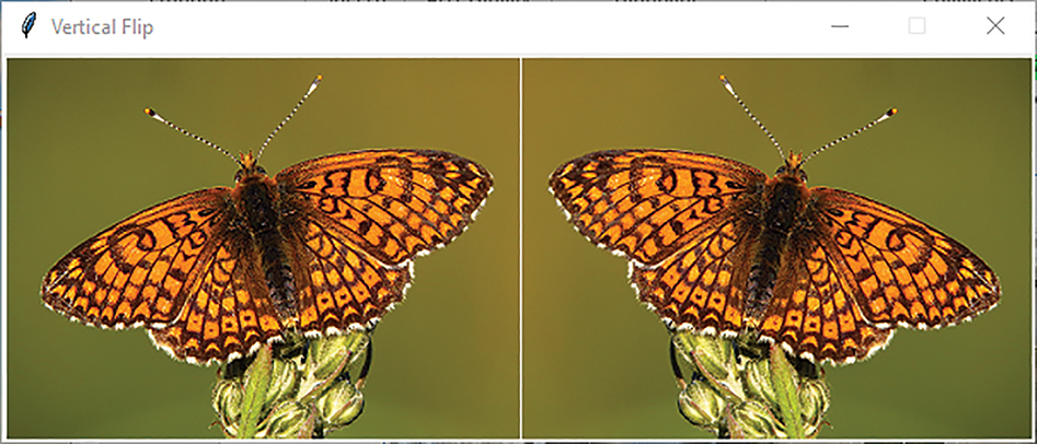
FIGURE 6.21 A flipped image.
© 2001–2019 Python Software Foundation. All Rights Reserved. Images A and B © Luka Hercigonja/Shutterstock.
6.5.4 Edge Detection
Our final image processing algorithm in this chapter is called edge detection. This image processing technique tries to extract feature information from an image by finding places in the image that have dramatic changes in color intensity values. For example, assume that we have an image containing two apples, one red and one green, that are placed next to each other. The border between a block of red pixels from the red apple and a block of green pixels from the green apple might constitute an edge representing the distinction between the two objects.
As another example, consider the black and white image shown in FIGURE 6.22. The left image contains three objects: a white square, a cloud, and a star. The right image shows the edges that exist in the image. Each black pixel in the edge image denotes a point where there is a distinct difference in the intensity of the original pixels. Finding these edges helps to differentiate between any features that may exist in the original image.
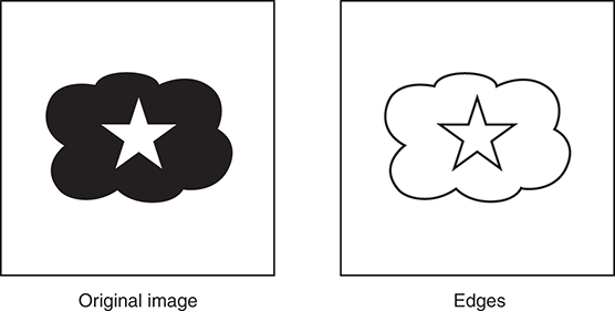
FIGURE 6.22 A simple edge detection.
Edge detection has been studied in great detail, and many different approaches have been developed to find edges within an image. In this section we describe one of the classic algorithms for producing the edges. The mathematics used to derive the algorithm are beyond the scope of this text, but we can easily develop the ideas and techniques necessary to implement the algorithm.
To find an edge, we need to evaluate each pixel in relation to the pixels around it. Since we are looking for places where the intensity on one side of the pixel is greatly different from the intensity on the other side, it will help us to simplify the pixel values. Our first step in discovering edges will be to convert the image to grayscale, so that we can think of the intensity of the pixel as the common color component intensity.
Recall that shades of gray are made from pixels with equal quantities of red, green, and blue. Each pixel can then be thought to have one of 256 intensity values.
As a means of looking for these intensity differences, we use the idea of a kernel, also known as a filter or a mask. Kernels can be used to weight the intensities of the surrounding pixels. For example, consider the 3-by-3 kernels shown in FIGURE 6.23. These “grids” of integer weights are known as Sobel operators, named after the scientist Irwin Sobel, who developed them for use in edge detection.
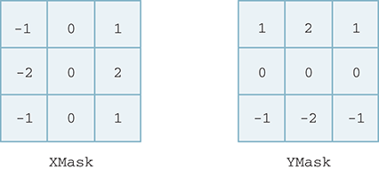
FIGURE 6.23 Kernel masks for convolving pixels.
We can use the left mask, labeled XMask, to look for intensity differences in the left-to-right direction of the image. You can see that the leftmost column of values is negative and the rightmost column is positive. Likewise, we can use the YMask to look for intensity differences in the up-and-down direction, as can be seen by the location of the positive and negative weights.
The kernels are used during convolution—a process in which pixels in the original image are mathematically combined with each mask. The result is then used to decide whether that pixel represents an edge.
Convolution requires both a mask and a specific pixel. The mask is “centered” on the pixel of interest, as shown in FIGURE 6.24. Each weight value in the mask then associates with one of the nine pixel intensities “under” the mask. The convolution process simply computes the sum of nine products, where each product is the weight multiplied by the intensity of the associated pixel. Thus, if you have a large intensity on the left side and a small intensity on the right (indicating an edge), you will get a weighted sum with a large negative value. If you have a small intensity on the left and a large intensity on the right, you will get a large positive weighted sum. Either way, a large absolute value of the weighted sum will indicate an edge. This same argument applies for the top-to-bottom split of the YMask.
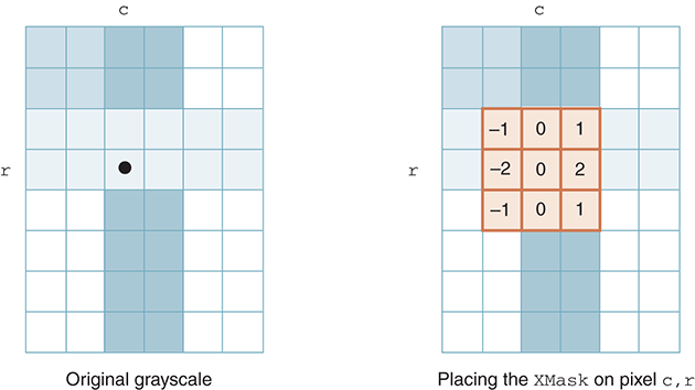
FIGURE 6.24 Using the XMask to convolve the pixel at c,r.
To implement convolution, we will first need to consider a way to store the kernels. Since kernels look very similar to images (that is, they are rows and columns of weights), it makes sense to take advantage of this structure. We will use a list of lists implementation for the kernel. For example, the XMask discussed earlier will be implemented as the list [ [-1,0,1],[-2,0,2], [-1,0,1] ]. The outer list contains three items, each of which represents a row in the kernel. Each row has three items, one for each column. Similarly, the YMask will be [ [1,2,1],[0,0,0],[-1,-2,-1] ].
Accessing a specific weight within a kernel will require two index values: one for the outer list and one for the inner list. Because we are implementing the outer list to be a list of three rows, the first index will be the row value. Once we select a row list, we can use the second index to get the specific column.
For example, XMask[1][2] will access the item in XMask indexed by 1, which is the middle row of the XMask. The 2 indexes the last item in the list, which corresponds to the last column. This access is for the weight stored in the middle row and last column of XMask.
We can now construct the convolve function. As noted earlier, the convolution process requires an image, a specific pixel within the image, and a kernel. The tricky part of this function is to align the kernel and the underlying image. An easy way to do this is to think about a mapping. The kernel row indices will run from 0 to 2, and likewise for the column indices. For a pixel in the image with index (column, row), the row indices for the underlying pixels will run from row - 1 to row + 1; for the columns, the indices will run from column - 1 to column + 1.
We will define the base index to be the starting index for the 3 × 3 grid of underlying image pixels. The base index for the columns will be column - 1 and the base index for the rows will be row - 1. As we process the pixels of the image, the difference between the current image row value and the base index for the rows will be equal to the row index needed to access the correct row in the kernel. We can do the same thing for the columns.
Once we have computed the index into the kernel, we can use that index to compute the product of the weight and the pixel intensity. We will first access the pixel and then extract the red component, which will be its grayscale intensity. Since we have already converted the image to grayscale, we can use any of the red, green, or blue components for the intensity. Finally, that product can be added to a running sum of products for all underlying pixels.
The complete convolve function is shown in LISTING 6.12. Note that the final step is to return the value of the sum.
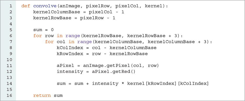
LISTING 6.12 Convolution for a specific pixel
Now that we can perform the convolution operation for a specific pixel with a kernel, we can complete the edge detection algorithm. The steps of the process are as follows:
Convert the original image to grayscale.
Create an empty image with the same dimensions as the original image.
Process each inner pixel of the original image by performing the following:
Convolve the pixel with the
XMask; call the resultgX.Convolve the pixel with the
YMask; call the resultgY.Compute the square root of the sum of squares of
gXandgY; call the resultg.Based on the value of
g, assign the corresponding pixel in the new image to be either black or white.
LISTING 6.13 shows the Python code that implements these steps. We begin by converting the original image to grayscale using the pixelMapper() function developed earlier in the chapter. This will allow for simple intensity levels within each pixel. We also need an empty image that is the same size as the original image. In addition, we will define a few data objects for use later. Because each pixel in the edge detection result will be either black or white, we create black and white tuples that can be assigned later in the process. Also, we need the list of lists implementation of the two kernels. These initializations are done on lines 3–8.
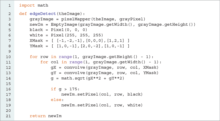
LISTING 6.13 The edge detection method
Now it is time to process the original pixels and look for an edge. As each pixel is required to have eight surrounding pixels for the convolution operation, we will not process the first and last pixel on each row and column. Thus, our nested iteration will start at one, not zero, and it will continue through height - 2 and width - 2, as shown on lines 10–11.
Each pixel will now participate in the convolution process using both kernels. The resulting sums will be squared and summed together, and in the final step we will take the square root (see lines 12–14).
The value of this square root, called g, represents a measure of how much difference exists between the pixel of interest and the pixels around it. The decision as to whether the pixel should be labeled as an edge is made by comparing g to a threshold value. It turns out that when using these kernels, 175 is a good threshold value for considering whether you have found an edge. Using simple selection, we will just check whether the value is greater than 175. If it is, we will color the pixel black; otherwise, we will make it white. FIGURE 6.25 shows the result of executing this function.
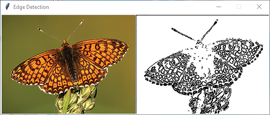
FIGURE 6.25 Running the edge detection algorithm.
© 2001–2019 Python Software Foundation. All Rights Reserved. Images A and B © Luka Hercigonja/Shutterstock.