
7.5 Implementing Cluster Analysis: Earthquakes
In the Bigger Data chapter, we worked with real data describing 501 earthquakes that occurred during a month in late 2018. Given the raw data, it might be difficult to see any type of pattern or similarity in this data set. However, if we extend our cluster analysis technique from the previous section, we might discover some interesting results.
7.5.1 File Processing
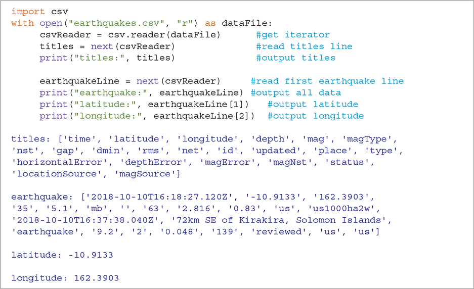
Our first problem will be to find a way to process and store the data contained in the data file so that we can use it in our clustering algorithm. Recall that in the earthquakes.csv file, the first line contains titles that identify each data item, like this:

Each succeeding line of the file describes one earthquake. The line for the first earthquake was the following:

This entry describes an earthquake of magnitude 5.1 that occurred at a depth of 35 kilometers in the general region of the Solomon Islands. The exact latitude (–10.9133) and longitude (162.3903) are also provided.
For this example we deploy our cluster analysis algorithm using the location data for each earthquake. In other words, we would like to see if some earthquakes are clustered in close proximity to one another. To do this, we need to understand how the location data is stored in the file and what it means.
Each earthquake is described by providing its exact location as a pair of values: longitude and latitude. The latitude values run north–south, with zero latitude being located at the equator. The north pole of the globe is +90, and the south pole is −90.
Likewise, the longitude values run west–east, with zero longitude being the prime meridian, an imaginary line that runs north–south through Greenwich, England. For latitudes in the far west, the measurement is −180; the far east measurement is +180, since the globe is assumed to be a full 360-degree circle on the equator.
Our data points now have two dimensions: a latitude and a longitude. Our previous description of the algorithm is still appropriate because, as you will recall, we went to the trouble of making the euclidD function work with multidimensional data points.
We can now work on extracting the necessary data from the file. Looking at the example line again shows us that for each earthquake, the data items are separated by a comma. We can easily extract the data values we want by using the csv module as shown in SESSION 7.3. Recall from Chapter 5 that the csv.reader method interprets the comma-separated values in the file, and that the next function returns the next line in the file.
SESSION 7.3 File processing for earthquake data
We can build the Python code using the framework from Session 7.3. After opening the file, we iterate through the lines and extract the latitude and longitude. LISTING 7.10 shows the readEarthquakeFile function, which creates a data dictionary of two-dimensional data points.
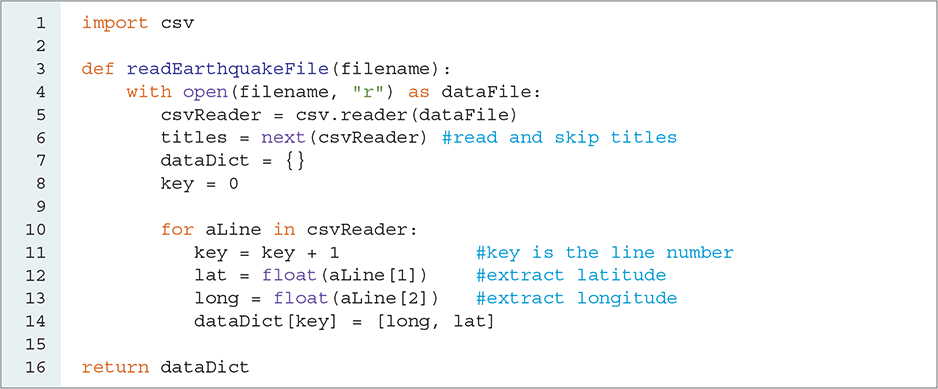
LISTING 7.10 Processing the earthquake data file
We continue to use the key as a way to refer to each unique line of the file. In this case, the dataDict dictionary associates the key with the longitude–latitude data point. Lines 12–13 extract the longitude and latitude data. Note that we need to convert these string values into floating-point numbers.
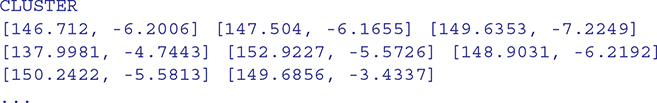
Once we have our data points, we can call our clusterAnalysis function. Remember that we need to make decisions about how many clusters we want to create and how many iterations should be used. Unfortunately, when we run our program, the output, a fragment of which is shown here, is difficult to understand. The reason for this lack of clarity is that our simple output mechanism displays the contents of each cluster by showing the data points.
7.5.2 Visualization
One more modification will make our results much more interesting. Instead of printing the longitudes and latitudes in long lists, we will use visualization to plot the positions of the earthquakes on a map of the world and show the clusters as points on that map. This process of “visualizing” the data can be quite useful, especially if we are looking for relationships that may not be readily apparent from long lists of data. It is common to look for some way to visualize the clusters.
As an example of this type of visualization, consider FIGURE 7.8, where the earthquake data has been processed using six clusters. Each earthquake is shown as a point on the map. In addition, the clusters are colored to distinguish one from the other. We can readily identify some relationships regarding where these earthquakes are taking place (although you likely knew this already).
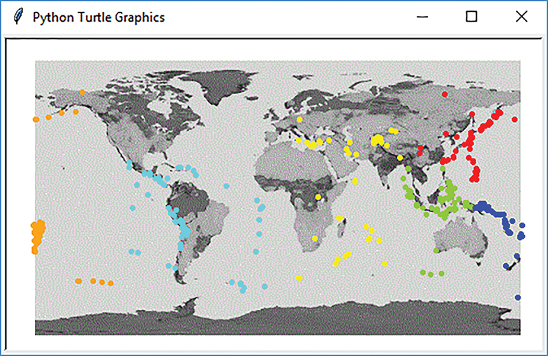
FIGURE 7.8 Plotting earthquakes to show clusters.
Map credit: NASA’s Goddard Space Flight Center. Image credit: Copyright © 2001–2019 Python Software Foundation. All Rights Reserved.
We can easily build this visualization by revisiting our old friend, the turtle module. The basic idea is to use the turtle to plot a colored “dot” at each earthquake location given by the longitude and latitude. The color will depend on the cluster to which the earthquake belongs. The challenging part is setting up the drawing window so that the map and the coordinates are consistent with our longitude and latitude values.
LISTING 7.11 shows a function to generate clusters and visualize them. First, we make use of the readEarthquakeFile, createCentroids, and createClusters functions. Once the clusters have been computed, we create a turtle called quakeT using the Turtle constructor. Looking again at Figure 7.8, you can see that the background of the turtle drawing window contains an image of the world. This image, stored in a file named worldmap.gif, is 448 pixels wide by 252 pixels high. By using the bgpic method (line 8), we can set this image as the background picture for the drawing window. Since we want the drawing window to include only the area of the map, we can then use the screensize method (line 9) to reset the width and height of the drawing window.
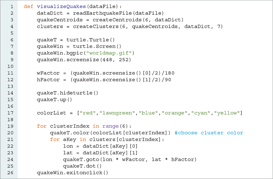
LISTING 7.11 Visualizing earthquake clusters
From our previous discussion of longitude and latitude, we know that the lower-left corner of the map should be location (−180, −90) and the upper-right corner should be (180, 90). We can “remap” our plotting by recognizing that the current lower-left corner is (−224, −126) and the upper-right corner is (224, 126). Thus, we simply compute multiplication factors for the width and the height (wFactor and hFactor in lines 11 and 12, respectively) and use them when we plot the longitude and latitude (line 24).
Lines 14–15 turn off the locational marker for the turtle and raise the turtle’s tail so that lines are not drawn as the turtle is moved from location to location. Finally, line 17 creates a list of colors that will be used to distinguish each cluster—red for the first cluster, lawngreen for the second, and so on.
We can now show the contents of each cluster by iterating through the clusters, processing each earthquake in the cluster. Line 20 sets the tail color by using clusterIndex as an index into the colorList. For each earthquake in the cluster, we extract the longitude and latitude data from the dataDict and use those two values as coordinates for the turtle. Once the turtle has been directed to the proper location, the dot method plots a point using the current tail color. Note that the number of colors in the colorList must be at least as large as the number of clusters being created so that each cluster gets a unique color.