6.3 Basic Image Processing
We now have all the tools necessary to do some simple image processing. Our first examples will perform color manipulations on an image. In other words, we want to take the existing pixels and modify them in some way to change the appearance of the original image. The basic idea will be to systematically process each pixel one at a time and perform the following operations:
Extract the color components.
Build a new pixel.
Place that pixel in a new image at the same location as in the original.
Once we see the general pattern, our options for image processing are endless. Note that all of the newly constructed images in this section will have the same dimensions as the original image.
6.3.1 Negative Images
When images are placed on film and then developed, a set of negatives is produced. A negative image is also known as a color-reversed image. In such an image, red becomes cyan, where cyan is the mixture of green and blue. Likewise, yellow becomes blue, and blue becomes yellow. Regions that are white turn black, black turns white, light turns dark, and dark turns light. This color reversal continues for all possible color combinations.
At the pixel level, the negative operation is just a matter of “reversing” the red, green, and blue components in that pixel. Thus, to create a negative pixel, we just subtract each of the red, green, and blue intensity values from 255. Since color intensity ranges from 0 to 255, a pixel with a large amount of a specific color—say, red—will have a small amount of that color in the negative. At the maximum, a pixel with a red intensity of 255 will have a red intensity of 0 in the negative. The color-reversed results can then be placed in a new pixel.
LISTING 6.1 shows a function that will take a Pixel as a parameter and return the negative pixel using the process just described. Note that the function expects to receive an entire Pixel; it then decomposes the color components, performs the subtractions, and builds and returns a new Pixel. We can easily test this function, as shown in SESSION 6.6.
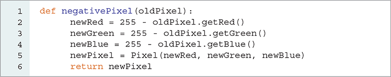
LISTING 6.1 Constructing a negative pixel
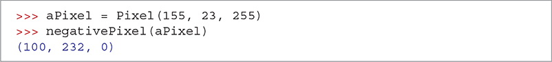
SESSION 6.6 Testing the negativePixel function
To create the negative image, we call the negativePixel function on each pixel. We then need to come up with a pattern that will allow us to process each pixel. To do so, we can think of the image as having a specific number of rows equal to the height of the image. Each row, in turn, has a number of columns equal to the width of the image. With this idea in mind, we can build an iteration that will systematically move through all of the rows and, within each row, will move through all of the columns. This gives rise to the notion of nested iteration—the placement of an iteration as the process inside of another iteration. In other words, for each pass of the “outer” iteration, the “inner” iteration will run to completion. The inner iteration will run from start to finish for each pass of the outer iteration.
As an example, consider the code fragment in SESSION 6.7 using for statements. The outer iteration moves over the list [0,1,2], which was produced by range(3). For each item in that list, the inner loop iterates over the characters 'c', 'a', 't'. As a consequence, the print function is called for each character in the string "cat" for each number in the list [0,1,2].
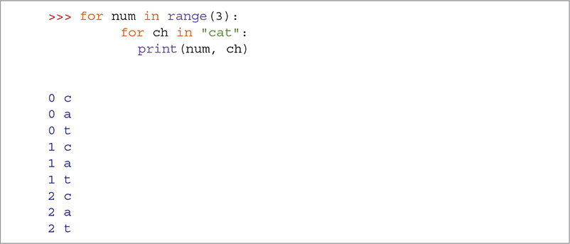
SESSION 6.7 Showing nested iteration with lists and strings
The resulting output shows nine lines. Each group of three represents one pass of the outer loop. Within each group, the value of num stays the same. For each value of num, the entire inner loop completes, and therefore each of the three characters of the string is output.
We can now apply this idea to the construction of a function to compute the negative of each pixel in an image (see LISTING 6.2). This function will take a single parameter that gives the name of a file containing an image. It will not return anything, but will simply display both the original image and the negative image side by side.
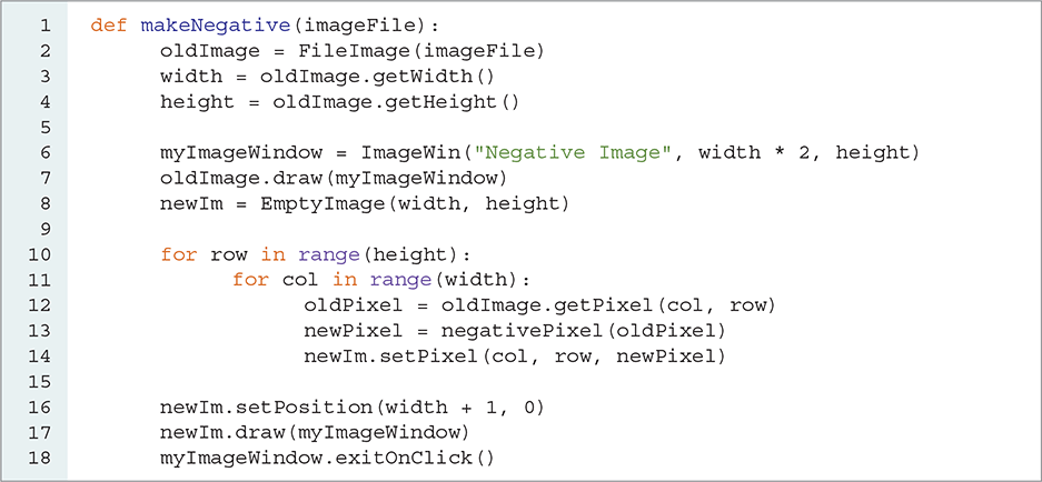
LISTING 6.2 Constructing a negative image
The first step (lines 2–8) is to get the width and height of the original image and create a window that has the same height but has twice the width as the original image, so that the negative image can be displayed next to the original. We then draw the original image in the window and create an empty image that has the same width and height as the original.
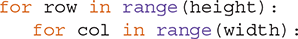
Using the idea of nested iteration (lines 10–14), we will first iterate over the rows, starting with row 0 and extending down to height-1. For each row, we will process all of the columns from 0 to width-1.
Each pixel is accessed by row and col. We can get the original color tuple at that location using the getPixel method (line 12). Once we have the original pixel, we can use the negativePixel function to transform it into the negative pixel. Finally, using the same row and col, we can place the new negative pixel in the new image (line 14) using the setPixel method. Once the iteration is complete for all pixels, the new image is drawn in the window. Note that we use the setPosition method to place the new image next to the original. FIGURE 6.4 shows the resulting images.
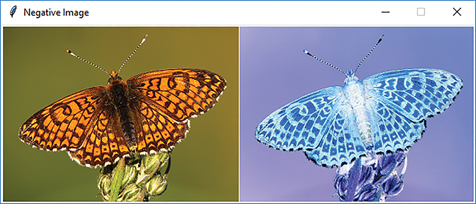
FIGURE 6.4 A negative image.
© 2001–2019 Python Software Foundation. All Rights Reserved. Images A and B © Luka Hercigonja/Shutterstock.
6.3.2 Grayscale
Another common color manipulation is to convert an image to grayscale, where each pixel will be a shade of gray, ranging from very dark (black) to very light (white). With grayscale, each of the red, green, and blue color components will take on the same value. In other words, there are 256 different grayscale color values ranging from darkest (0, 0, 0) to lightest (255, 255, 255). The standard color known as “gray” is typically coded as (128, 128, 128).
Our task, then, is to convert each color pixel into a gray pixel. The easiest way to do this is to consider that the intensity of each red, green, and blue component needs to play a part in the intensity of the gray image. If all the color intensities are close to zero, the resulting color will be very dark, which should in turn show as a dark shade of gray. In contrast, if all of the color intensities are closer to 255, the resulting color will be very light and the resulting gray should be light as well.
This analysis gives rise to a simple but accurate formula for converting a color image to grayscale: We will simply take the average intensity of the red, green, and blue components. This average can then be assigned to all three color components in a new pixel, resulting in a shade of gray. LISTING 6.3 shows a function, similar to the negativePixel function described previously, that takes a Pixel object and returns the grayscale equivalent. SESSION 6.8 shows the function in use.
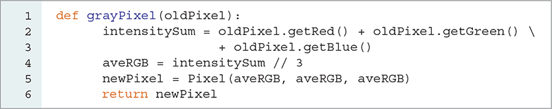
LISTING 6.3 Constructing a grayscale pixel
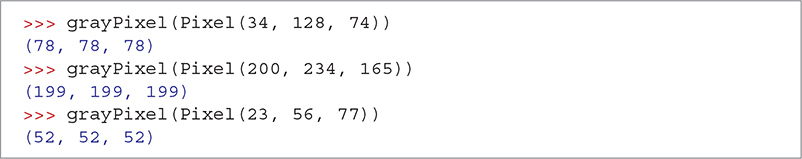
SESSION 6.8 Testing the grayPixel function
Now the process of creating a grayscale image can proceed in the same way as described for creating the negative image (see LISTING 6.4). After opening and drawing the original image, we create a new, empty image. Using nested iteration, we process each pixel, this time converting the pixel to the corresponding grayscale value (line 13). The final image is shown in FIGURE 6.5.
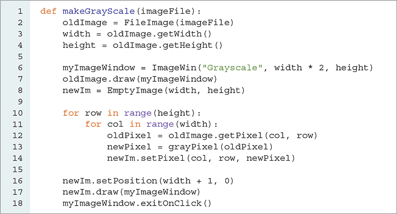
LISTING 6.4 Constructing a grayscale image
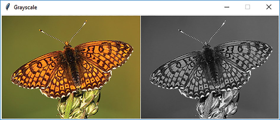
FIGURE 6.5 A grayscale image.
© 2001–2019 Python Software Foundation. All Rights Reserved. Images A and B © Luka Hercigonja/Shutterstock.
We developed the previous examples by continually building upon and extending a framework of simple ideas. We started with the pixel, then created a function to transform the color components of a pixel, and finally applied that function to all of the pixels in the image. This type of stepwise construction is a methodology that is widely used in writing computer programs. Building upon those functions that already work to create more complex functionality that can again be used as a foundation for additional functions allows programmers to be very efficient. We take this one step further in the next section.
6.3.3 A General Solution: The Pixel Mapper
If you compare the Python listings for the makeGrayScale and makeNegative functions, you will notice quite a bit of redundancy. In fact, the same steps were followed with only one exception—namely, the function that was called to map each original pixel into a new pixel. This similarity causes us to think that we could factor out the code that is the same and create a more general Python function. This is another example of using abstraction to solve problems.
FIGURE 6.6 shows how such a function might be constructed. We will create a function called pixelMapper that will take two parameters, an original image and an RGB function. The pixelMapper function will transform the original image into a new image using the RGB function. After applying the RGB function to every pixel, we will return the transformed image. In this way, we can create a single function that is capable of transforming an image given any function that manipulates the color intensities of a single pixel.
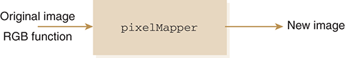
FIGURE 6.6 A general pixel mapping function.
To implement this general pixel mapper, we need to be able to pass a function as a parameter. Up to this point, all of our parameters have been data objects such as integers, floating-point numbers, lists, tuples, and images. The question we must consider here is whether there is any difference between a function and a typical data object.
The answer to this question is simple: There is no difference. To understand why, we will first look at a simple example. The function squareIt takes a number and returns the square.
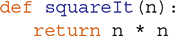
We can invoke the squareIt function with the usual syntax (see SESSION 6.9), placing the actual value to be squared as a parameter. However, if we evaluate the name of the function without invoking it (without the parameters in parentheses), we notice that the result is a function definition. The name of a Python function is a reference to a data object—in particular, a function definition (see FIGURE 6.7). Note that the strange-looking number, 0x0000022740D68E18, is actually the address where the function is stored in memory.
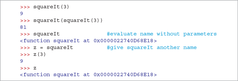
SESSION 6.9 Evaluating the squareIt function
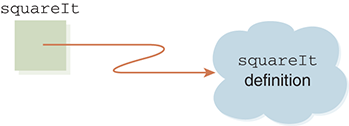
FIGURE 6.7 A function is a data object.
Since a function is simply another data type, you might wonder which kinds of operators you can use with it. In fact, you can use only two operators with a function. The parentheses are actually an operator that tells Python to apply the function to the supplied parameters. In addition, because a function is an object, you can use the assignment operator to give a function another name, as shown in Session 6.9. Note that now the variable z is a reference to the same data object as squareIt and can be used with the parentheses operator.
As any Python object can be passed as a parameter, it is certainly possible to pass the function definition object. We just need to be careful not to invoke the function prior to passing it. To illustrate this point (SESSION 6.10), we create a simple function called test that expects two parameters: a function object and a number. The body of test will invoke the function object using the number as a parameter and return the result.
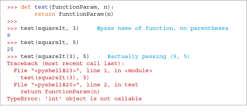
SESSION 6.10 Using a function passed as a parameter
We can then use our test function by passing the squareIt function definition. In addition, we will pass the integer 3. Remember, when we pass the function definition object, we do not include the parentheses pair. FIGURE 6.8 shows the references immediately after test has been called and the parameters have been received. A copy of the reference to the actual parameter squareIt is received by functionParam, and n contains a reference to the object 3.
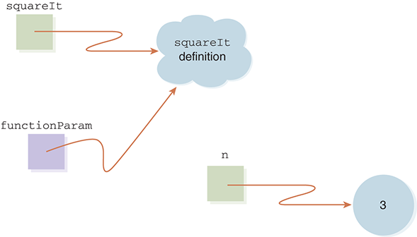
FIGURE 6.8 Passing the method and an integer.
The statement return functionParam(n) will cause the function referred to by functionParam to be invoked on the value of n. In this case, since functionParam is a reference to squareIt, the squareIt function will be invoked with the value of 3. The next example shows the result of passing 5 instead of 3. Note the error message that appears at the end of the session when we call the squareIt function instead of passing the definition.
With these mechanics in place, it is now possible to create an implementation for our general pixelMapper function (see LISTING 6.5). Recall that this function takes two parameters: a FileImage and an RGB function. Lines 3–5 construct a new empty image that is the same size as the original image. Line 10, which is inside our nested iteration, does most of the work. The rgbFunction parameter is applied to each pixel from the original image and the resulting pixel is placed in the new image. Once the nested iteration is complete, we return the new image.
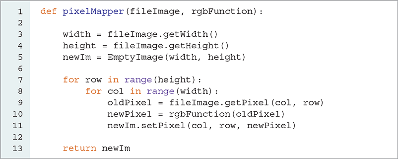
LISTING 6.5 A general pixel mapping method
We can complete our example by calling the pixelMapper function using one of our RGB functions from the previous sections. LISTING 6.6 shows the main function, generalTransform, that sets up the image window and loads the original image. Line 9 invokes pixelMapper using the grayPixel function. The result is identical to that shown in Figure 6.5.
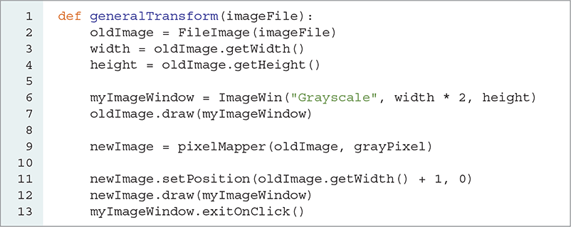
LISTING 6.6 Calling the general pixel mapping function