1.5 Python Overview
In this text, the language you will use to write your computer programs is called Python. Why did we choose Python instead of a language like C++ or Java? The answer is simple: We want you to focus on learning the problem-solving strategies and techniques that a computer scientist uses. Programming languages are tools, and Python is a good beginning tool. Languages like Java and C++ are fine tools as well, but they require you to keep track of many more details than Python does.
The best way to learn Python is to try it out—so let’s get started. Python is free to download and install. You will find detailed instructions on installing Python on various operating systems at www.python.org. In fact, python.org is a good resource for learning more about Python and its many libraries, which are prewritten Python code we can incorporate into our programs.
After installing Python, the first thing you do is start the Python interpreter. Depending on your operating system, there are any number of ways to do this. For example, you might start a program called IDLE—named after Eric Idle of Monty Python fame. Or you might just type Python at the command prompt. No matter how you start it, you will know you are successful when you see a window such as the one shown in FIGURE 1.3. In this case, we have started the Python interpreter on a Windows 10 computer.
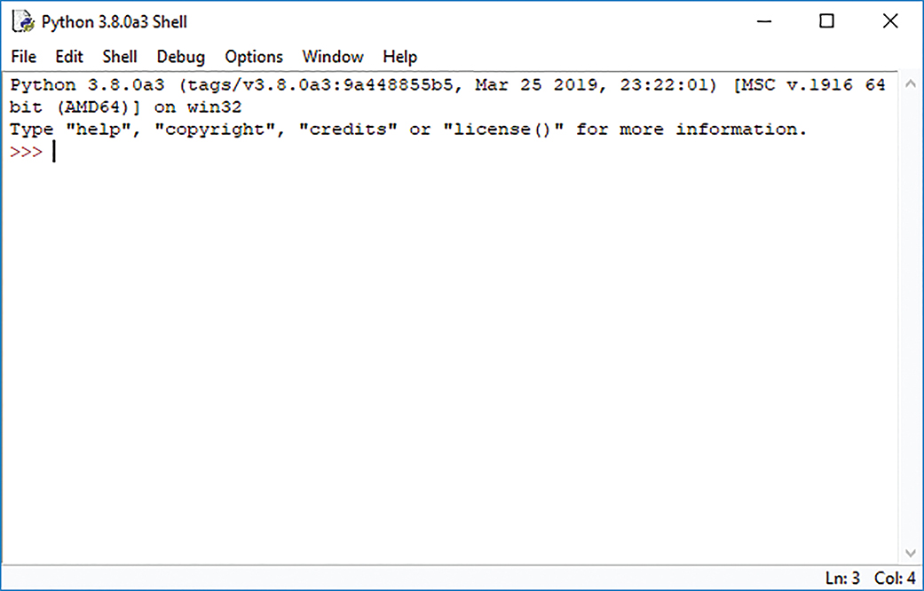
FIGURE 1.3 The Python IDLE interpreter.
As you progress through this chapter, you will see that example programs appear in boxes called listings, and commands that you can type interactively at the Python shell appear in boxes called sessions. Whenever you see a session box, we strongly encourage you to try the session for yourself. Also, once you have typed in the example shown in the session, feel free to try some variations to find out for yourself what works and what does not.
As we begin to explore Python, we will answer three important questions you should ask about any programming language:
▶ What are the primitive elements?
▶ How can we combine the primitive elements?
▶ How can we create our own abstractions?
1.5.1 Primitive Elements
At the deepest level, the one primitive element in Python is the object. Like you, Python thinks of the things in its world as objects. If you look around your world, you will see many objects: pencils, pens, your chair, a computer. Python even considers numbers to be objects—an idea that may be a bit confusing to you, because you probably don’t think of numbers as objects. But Python does, and we’ll see why this is important shortly.
Python classifies the different kinds of objects in its world into types. Some of the easiest types to work with are numbers. Python knows about several different types of numbers:
▶ Integer numbers
▶ Floating-point numbers
▶ Complex numbers
Integer Numbers
Integers are the whole numbers that you learned about in math class. We can do a lot with Python just using integers. For starters, we can use the Python interpreter we started a few moments ago as a calculator. Notice that Python displays >>>. These three characters, which are called the Python prompt, indicate that the Python interpreter is ready for you to type an expression. Let’s try a few mathematical expressions. Type in the following examples using the Python interpreter. After you have typed in an expression, press the enter or return key to see the result.
The examples in SESSION 1.1 illustrate some very important Python concepts that you should become familiar with as soon as possible. The first concept is Python’s read–eval–print loop.
SESSION 1.1 Simple integer math
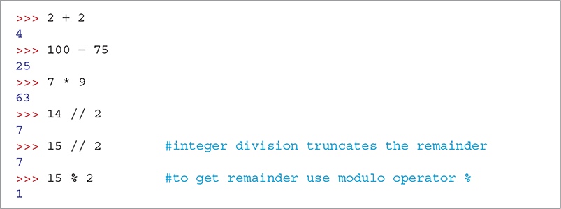
At a high level, the Python interpreter is really very simple. It does three things over and over again: (1) read, (2) evaluate, and (3) print. These are illustrated in FIGURE 1.4.
FIGURE 1.4 The read–eval–print loop in Python.
First, Python reads one line of input. In the first example, Python reads 2 + 2, then it evaluates the expression 2 + 2 and determines that the answer is 4. Finally, Python prints the resulting value of 4. After displaying the result, Python prints the characters >>> to show you that it is waiting to read another expression.
In general, a Python expression is a combination of operators and operands. TABLE 1.1 shows Python’s arithmetic operators.
TABLE 1.1 Python’s Arithmetic Operators |
|
|---|---|
| Operator | Operation |
| + | Addition |
| − | Subtraction |
| * | Multiplication |
| // | Integer division |
| / | Floating-point division |
% |
Modulo (remainder after division) |
| ** | Exponentiation |
When we evaluate an expression, we get a result. In the examples in our Python session, some of the operators are familiar mathematical operators: ‘+’ and ‘−’. Although you may be more used to × and ÷ for multiplication and division, you will not find those symbols on a standard keyboard, so Python, like almost all programming languages, uses “*” for multiplication and “/” or “//” for division.
One thing that may surprise you in the example is the result of the expression 15 // 2. Of course, we all know that 15 divided by 2 is really 7.5. However, because both operands are integer objects and // is the integer division operator, Python produces an integer object as a result. Integer division works like the division you learned when you were young: 15 divided by 2 equals 7, remainder 1. You can find the remainder part of the result by using the modulo operator (%). For example, 15 % 2 evaluates to the remainder value of 1.
Let’s try some more calculations. Type the expressions in SESSION 1.2 into the Python interpreter.
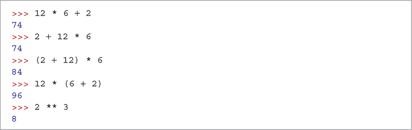
SESSION 1.2 More numeric calculations
Here we are mixing multiplication and addition. As shown in the first two calculations, the order in which we type the expressions does not make a difference in the result. The reason for this is that Python performs all multiplications and divisions before performing any additions and subtractions. We can override those rules by putting parentheses around any calculation we want to perform first, as shown in the third and fourth expressions.
Finally, we introduce the exponentiation operator (**) for raising a number to a power. In this case, we raise 2 to the third power, yielding 8.
TABLE 1.2 summarizes the order in which Python performs calculations. Operators are evaluated in order from top to bottom; operators at the same level are evaluated from left to right as they occur in the expression, except for exponentiation, which is evaluated from right to left.
TABLE 1.2 Python’s Order of Operations |
||
|---|---|---|
| Operators | Operations | Evaluation Order |
| ( ) | Parentheses | Left to right |
| ** | Exponentiation | Right to left |
| * // / | Multiplication and division | Left to right |
| + = | Addition and subtraction | Left to right |
Floating-Point Numbers
Integer division is useful in some cases, but it can also trip you up. What if you want to divide 15 by 2 and get 7.5 as the answer? To get the result as a floating-point number, you must use the floating-point division operator ‘/’.
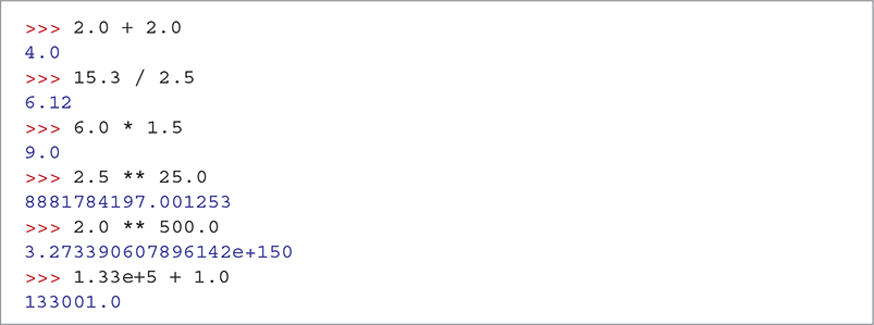
In Python, you can tell the difference between a floating-point number and an integer because a floating-point number has a decimal point. Floating-point numbers are Python’s approximation of what you called real numbers in math class. We say that floating-point numbers are an approximation because, unlike real numbers, floating-point numbers cannot have an infinite number of digits following the decimal point. This is because of the way floating-point numbers are stored in the computer’s memory. SESSION 1.3 presents some examples of calculations using floating-point numbers.
SESSION 1.3 Floating-point math
Notice that when the operands are floating-point numbers, the result is a floating-point number including the remainder as a fractional part. You should also notice that when the result of a floating-point operation gets really big, Python uses scientific notation to express the results. Finally, notice that you can use scientific notation for a floating-point number in a Python expression.
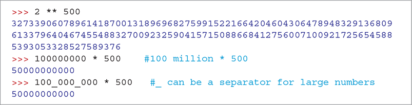
Although 3.273e + 150 is a good approximation, we know that there are not really 147 zeros in the result. One of the disadvantages of using scientific notation is that you lose some precision in your result. If you want to get very exact results, integers allow us to perform calculations to virtually unlimited precision. SESSION 1.4 shows the real value of 2**500 using integers.
SESSION 1.4 The use of integers to obtain very precise answers for large numbers
When typing large integers, you might be tempted to insert commas between groups of 3 numbers—for example, 100,000,000. Unfortunately, Python does not allow commas to be inserted into integers. Session 1.4 shows that Python does allow an underscore (_) to act as a visual separator for typing large numbers. The underscore is not considered part of the integer, but simply acts as an aid in typing large numbers.
Complex Numbers
The final primitive numeric type in Python is the complex number. As you may remember, complex numbers have two parts to them: a real part and an imaginary part. In Python, a complex number is displayed as real + imaginary j. For example, 5.0 + 3j has a real part of 5.0 and an imaginary part of 3. Although we mention complex numbers here to give you a complete list of the numeric primitives, we will not go into any additional details at this point.
Mixing Numeric Types
What happens when we mix numbers of different types in one calculation? Let’s look at the examples shown in SESSION 1.5 to find out.
SESSION 1.5 Mixing integers and floating-point numbers
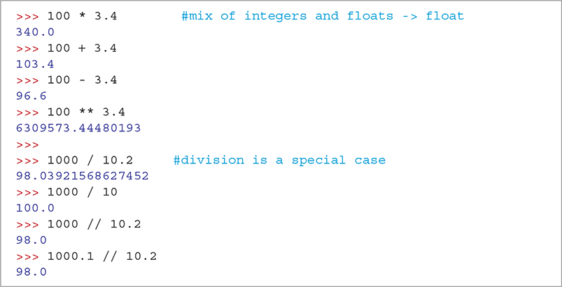
As you can see from Session 1.5, when you mix floating-point numbers with integers with the arithmetic operators other than division, the result will be a floating-point number.
For division, however, the result depends on which division operator you use. When you use the floating-point division operator (/), regardless whether the operands are integers or floating-point numbers, the result will be a floating-point number. When you use one or more floating-point numbers with the integer division operator (//), the result is also a floating-point number, but with the fractional part truncated.
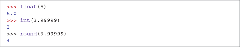
As shown in SESSION 1.6, you can also tell Python to explicitly convert a number to either an integer or a floating-point number by using the int or float functions. These functions are built-in Python code that operate on a value you put into parentheses after the function name. For example, float(5) will convert the integer 5 to the floating-point number 5.0. Conversely, int(3.99999) will convert the floating-point number 3.99999 to the integer 3. When converting floating-point numbers to integers, Python always truncates the fractional part of the number. If you want to convert a floating-point number to the nearest integer, you can use the built-in round function. For example, round(3.99999) will round the floating-point number 3.9999 to 4.
SESSION 1.6 Converting between integers and floating-point numbers
These numeric type conversion functions are summarized in TABLE 1.3.
TABLE 1.3 Python’s Functions for Converting Between Numeric Types |
|
|---|---|
| Function | Description |
float(i) |
Converts the integer i to a floating-point number. |
int(f) |
Converts the floating-point number f to an integer. Any fractional part is truncated. |
round(f) |
Converts the floating-point number f to the closest integer. |
In summary, we have seen that Python supports several types of primitive objects in the number family: integers, for ordinary simple math, when precision is required, or when dealing with very large numbers; and floating-point numbers, for working with scientific applications or accounting applications where we need to keep track of dollars and cents. At this point, however, Python is nothing more than a calculator. In the next section, we add some Python primitives that will give us a lot more power.
1.5.2 Naming Objects
Very often we have an object that we would like to remember. Python allows us to name objects so that we can refer to them later. For example, we might want to use the name pi rather than the value 3.14159 in a mathematical expression. We might also want to give a name to a value that we will use multiple times rather than recalculate it each time.
In Python, we can name objects using an assignment statement. A statement is like an expression except that it does not produce a value for the read–eval–print loop to print. An assignment statement has three parts: (1) the left-hand side, (2) the right-hand side, and (3) the assignment operator (=). The right-hand side can be any Python expression, and the left-hand side is the name to which we want to assign the result of evaluating the expression.

When the Python interpreter evaluates an assignment statement, it first evaluates the expression that it finds on the right-hand side of the equals sign. Once the right-hand side expression has been evaluated, the resulting object is referred to using the name found on the left side of the equals sign. In computer science, we call these names variables. More formally, we define a variable to be a named reference to a data object. In other words, a variable is simply a name that allows us to locate a Python object.
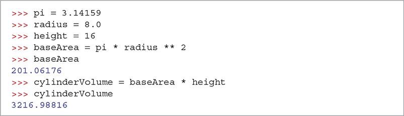
Suppose we want to calculate the volume of a cylinder for which the radius of the base is 8 cm and the height is 16 cm. We will use the formula volume = area of base * height. Rather than calculate everything in one big expression, we will divide the work into several assignment statements. First, we will name the numeric objects “pi,” “radius,” and “height.” Next, we will use the named objects to calculate the area of the base and finally the volume of the cylinder. SESSION 1.7 shows how we use this sequence of assignment statements and Python arithmetic to solve our problem.
SESSION 1.7 Calculating the volume of a cylinder with assignment statements
After studying Session 1.7, you may have some questions:
▶ How is the use of the equals sign in Python different from what you learned in math class?
▶ If you change the value for
baseArea, willcylinderVolumeautomatically change?▶ Why doesn’t Python print out the value of
piafter the first assignment statement?▶ Which names are legal in Python?
Let’s look at these questions one at a time. The equals sign in Python is very different from the symbol that you learned in math class. In fact, you should think of it not in terms of equality, but rather as the assignment operator, which has the job of associating a name with an object. FIGURE 1.5 illustrates how names are associated with objects in Python. All the names and objects in this figure come from Session 1.7. The relationships between names and the objects they reference are indicated by the arrows between them.
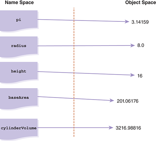
FIGURE 1.5 A reference diagram illustrating simple assignment in Python.
Another way of thinking about assignment is to imagine that an assignment statement is like taking a sticky label with a name written on it and attaching it to an object. You know that you can put more than one sticky label on an object in the real world, and the analogy holds true in the Python world as well: A Python object can have more than one name. For example, suppose you made the following additional assignment: x = 8.0. After executing that statement, you could add another label called x with another arrow pointing at the object 8.0, as shown in FIGURE 1.6.
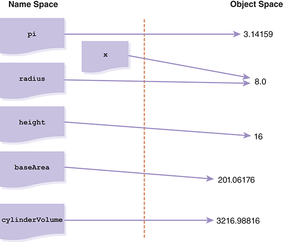
FIGURE 1.6 Reference diagram after x = 8.0.
Variables can take the place of the actual object in a Python expression. When Python evaluates the expression pi * radius ** 2, it first looks up pi and radius to see which objects they refer to; it then substitutes their values into the expression. The expression thus becomes 3.14159 * 8.0 ** 2. Next, Python evaluates 8.0 ** 2 to get an intermediate result of 64.0. Python then evaluates 3.14159 * 64.0 to get the value 201.06176. After the right-hand side of the expression is evaluated, Python assigns the name baseArea to 201.06176. Similarly, Python evaluates the expression baseArea * height by substituting the value 201.06176 for baseArea and multiplying by 16. Then Python assigns the name cylinderVolume to the value 3216.98816.
Let’s look at one more example using assignment. Consider the Python statements in SESSION 1.8.
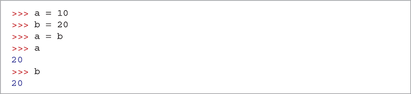
SESSION 1.8 Python evaluates assignment statements in sequence
After these three assignment statements, what object does a refer to? To answer this question, it is important to recognize that Python evaluates the statements from top to bottom, one after another. Let’s rephrase what is going on in the order that Python performs its work.
Assign the name
ato the integer object10.Assign the name
bto the integer object20.Find the object named
b, then assign the nameato that object.
The answer to our question is that a now refers to the object 20. This is shown in FIGURE 1.7. In addition, because we have not changed what b refers to since the original assignment, b continues to refer to the object 20. If you are confused by this example, try to draw the reference diagram yourself one step at a time.
FIGURE 1.7 Result of assignment a = b.
Now that you understand more about the assignment operator, you will appreciate that attaching the name baseArea to a different object will have no impact on the name cylinderVolume. If you want the new value for baseArea to affect the value of cylinderVolume, you will need to ask Python to re-execute the statement cylinderVolume = baseArea * height with the new value for baseArea.
Since assignment is a statement rather than an expression, it does not return a value. In consequence, there is nothing for the read–eval–print loop to print out. That is why you do not see any output following the assignment statements in Sessions 1.7 and 1.8.
A name on a line all by itself is a very simple Python expression. Notice that just typing a name causes Python to find the value for the object and return it as the result of the expression. You can see this in Session 1.7 when we type baseArea and cylinderVolume, and at the end of Session 1.8 when we type a and b. Python responds by printing their values.
There are several important rules to remember about naming things in Python. Names can include any letter, number, or an _ (underscore). Names must start with either a letter or an _. Python is case-sensitive, which means that the names baseArea, basearea, and BaseArea are all different.
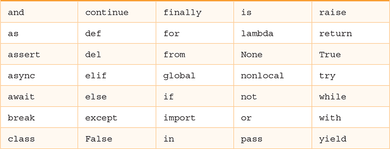
Some names are reserved by Python for its own use. These keywords correspond to important Python capabilities that you will learn about. TABLE 1.4 lists all of Python’s reserved keywords. Again, these reserved words are case-sensitive. For example, True is a reserved word, but true is not. To avoid confusion, it is a good programming practice not to choose names that are identical to the reserved words, except for case.
TABLE 1.4 Python’s Reserved Keywords |
|---|
|
1.5.3 Abstraction
Abstraction is defined as a concept or idea not associated with any specific instance. For example, you can think of mathematical functions on your calculator such as square root, sine, and cosine as abstractions. These functions can calculate a value for any number, but the method of calculating a square root is independent of the particular number. From that perspective, we can think of a function that calculates a square root as being the general idea. The square root function works equally well for all numbers because it is a general function. We do not have a special square root function for each possible number, just one function that works for all numbers.
One way of thinking about functions is as a “black box.” You send information into the black box on one side and new information comes out on the other side. You don’t know exactly what goes on inside the box, but you do know the behavior that the box should exhibit. FIGURE 1.8 illustrates this concept for the square root function.
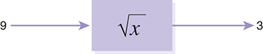
FIGURE 1.8 A black box view of the square root function.
The Python language contains many such abstractions. Many of the new things we will see in Python are, in fact, abstractions built using the Python primitives we have already talked about or will talk about later. In other words, much of Python is written in Python.
The turtle Module
Many of the additional parts of Python functionality are found in modules—prewritten Python code that implements an abstraction designed to make programming easier. To apply the power of a module, you have to tell Python to load the module you want. The statement you need to use to load a module is import modulename.
When you import a module, an object is created inside Python. That object has the type module and has a name attached to it that matches the name you used on the import line. Every object in Python has three important characteristics: (1) an identity, (2) a type, and (3) a value. In addition, some Python objects have special values called attributes, and some Python objects also have methods, which are bits of Python code that allow us to ask the object to do something interesting. Let’s look at a simple example before we go any further.
The example we will use is the turtle module, which provides us with a simple graphics programming tool known as a turtle. Very simply, a turtle is an object that we can control. A turtle can move forward or backward, and it can turn in any direction. When a turtle moves, it draws a line if its tail is down. A turtle is a Python object that has both attributes and methods. Some of the attributes of a turtle are shown in TABLE 1.5.
TABLE 1.5 Turtle Attributes |
|
|---|---|
| Position | The coordinates of the turtle on the screen |
| Heading | The direction the turtle is facing |
| Color | The color of the turtle |
| Tail position | The turtle’s tail can be up or down |
The methods of the turtle are summarized in TABLE 1.6. The second column is titled “Parameter(s).” Functions and methods are abstractions of generalized behaviors. Just as mathematical functions like cos(20) or ![]() take parameters, Python functions and methods may also accept parameters. Parameters are the way we tell the function specifically what it should do. If you see the Python keyword
take parameters, Python functions and methods may also accept parameters. Parameters are the way we tell the function specifically what it should do. If you see the Python keyword None in the Parameter column, that means that the method does not need any parameters to do its job.
TABLE 1.6 Summary of Simple Turtle Methods |
||
|---|---|---|
| Name | Parameter(s) | Description |
Turtle |
None | Creates and returns a new turtle object |
forward |
Distance | Moves the turtle forward |
backward |
Distance | Moves the turtle backward |
right |
Angle | Turns the turtle clockwise |
left |
Angle | Turns the turtle counterclockwise |
up |
None | Picks up the turtle’s tail |
down |
None | Puts down the turtle’s tail |
pencolor |
Color name | Changes the color of the turtle’s tail |
fillcolor |
Color name | Changes the color that the turtle will use to fill a polygon |
color |
Color name | Changes the color of the turtle’s tail and the color the turtle will use to fill a polygon |
heading |
None | Returns the current heading |
position |
None | Returns the current position |
goto |
x, y |
Moves the turtle to position x, y |
begin_fill |
None | Remembers the starting point for a filled polygon |
end_fill |
None | Closes the polygon and fills it with the current fill color |
dot |
None | Leaves a dot at the current position |
To start, we will just concern ourselves with a few of the turtle methods. For example, we can tell the turtle to go forward, go backward, turn left, turn right, or tell us its position. The turtle has a tail that can be up or down. When the tail is down and the turtle moves, it draws a line. If the tail is up and the turtle moves, nothing is drawn. SESSION 1.9 shows a Python session in which we create a turtle object and try out some of the turtle’s capabilities.
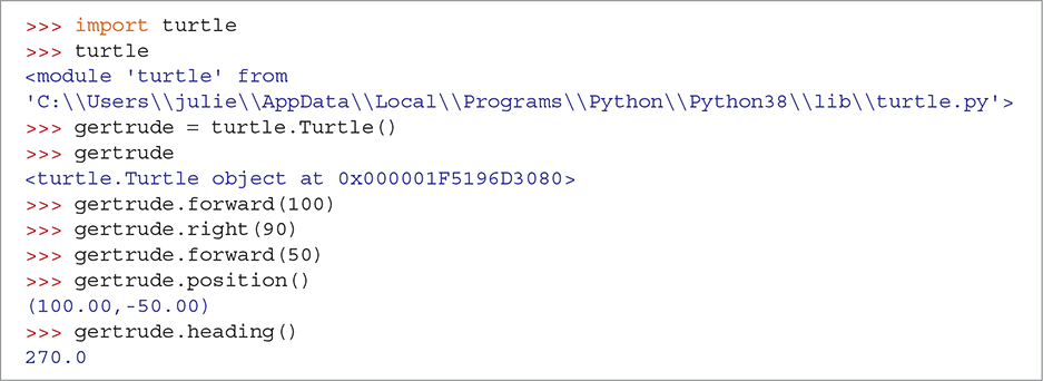
SESSION 1.9 Using the turtle module
Let’s look at this example line by line. In line 1, we use an import statement to load the turtle module. In line 2, we ask Python to evaluate the name turtle. Python rewards us by telling us the identity of the object to which turtle is assigned. That identity indicates the location of the Python code for the module. This location will vary according to the kind of computer you are using and where you installed Python. If we were really adventurous, we could go there and look at the turtle methods that are stored in the turtle.py file.
Once we have the turtle module loaded, we can start to use the methods in the module to do something interesting. In the fifth line we have an assignment statement, through which we make a new Turtle object and give it the name gertrude.
If you are typing this session interactively as you are reading, you will see that when a turtle is created, a new window, shown in FIGURE 1.9a, appears on the screen. The arrow in the middle of the screen represents the turtle. When a turtle is first created, it is at position (0.0, 0.0) in the middle of the window. The turtle’s initial heading is 0.0 degrees, or straight to the right. The color attribute for the new turtle is black, and the tail is down. As you move the turtle around, it remembers its latest position, the direction in which it is facing, and the status of its tail (up or down).
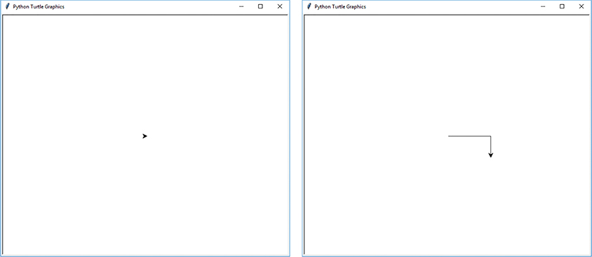
FIGURE 1.9 Using turtle graphics. (a) The turtle when it is first created. (b) The turtle after some movements.
© 2001–2019 Python Software Foundation; All Rights Reserved.
Before we go any further with this example, we need to explain the fifth line in more detail. Notice that the expression turtle.Turtle() contains a new operator—the dot (.). The dot operator tells Python to look up the name right in front of the dot and return the object it names, a process referred to as dereferencing. In this case, the dereferencing operation allows Python to find the turtle module. Once we have the module, Python looks within the module for the name to the right of the dot. In this case, Python looks for the Turtle method. A good way to think of this is that Turtle is Python code “inside” the turtle module. So the dot operator gets us to the turtle module, and then inside the turtle module we find the object named Turtle.
As we can see, turtle.Turtle() is a method that creates a new object. Note that the Turtle method does not take any parameters; nevertheless, we need to include the parentheses when calling a method, even if they are empty. The type of the new object created is Turtle. A method that creates a new object is called a constructor. New turtle objects that we construct are called instances of the type Turtle.
The next two lines simply demonstrate that when you evaluate a name that corresponds to a more complicated object, Python returns its representation of that object. Unlike for a number, where the representation is self-evident, a turtle’s representation gives you a unique identification for the object. In this case, we see that gertrude is <turtle.Turtle object at 0x000001F5196D3080>. To be even more specific, the result tells us that the type of gertrude is turtle.Turtle. Furthermore, our turtle can be found at location 0x000001F5196D3080 in the computer’s memory.
Now that we have our new turtle object named gertrude, the next three lines instruct gertrude to do some drawing. As you might guess, the line gertrude.forward(100) causes the turtle to move forward 100 units. Once again, the dot notation is very important to understanding how Python interprets the statement. First, the dot tells Python to dereference the name gertrude. When Python finds the object, it evaluates the method forward that is “inside” the turtle. The forward method knows that it needs to move forward 100 units because we pass it a parameter of 100. In this case, we want gertrude to move forward 100 units; then turn right 90 degrees; and then move forward again, but this time by only 50 units. If you run this example on your own, your window should look like FIGURE 1.9b.
The last four lines of Session 1.9 show that we can also use methods to ask the turtle for information about itself. First, we ask gertrude to tell us its location with the method call gertrude.position(). gertrude replies that the turtle is at (100.0, −50.0). What is actually happening is that the position() method returns the value (100.0, −50.0), and the print part of the read–eval–print loop prints out that value. All functions can return values, and those values can then be included in Python expressions. The fact that the position method returns a value is no different than the cosine function returning a value. Similarly, the heading() method tells us that gertrude is currently facing 270.0 degrees.
In the world of our turtle, the coordinates (0.0, 0.0) are in the center of the window. The x coordinate grows in a positive direction as the turtle moves toward the right. If the turtle moves toward the left side of the window, the x coordinate gets smaller and becomes negative to the left of the middle of the window. Similarly, the y coordinate grows as the turtle moves toward the top of the window, but gets smaller as the turtle moves toward the bottom and becomes negative below the middle of the window. One pixel on your computer screen corresponds to 1 unit of turtle movement. The turtle’s heading varies from 0 to 359, moving counterclockwise around the window. If the turtle’s heading is 0.0 degrees, it is facing to the right; 90.0 degrees is up, 180.0 degrees is to the left, and 270.0 degrees is down.
The turtle module has many other methods. Table 1.6 shows just a few of them. We’ll introduce additional methods as we have need for them in future examples.
Writing Your Own Functions
We are not limited to the functions that the authors of Python have given us. We, too, can write our own functions to add our own abstractions to the Python language. In fact, functions are just another kind of Python object with several special capabilities. We define a function in Python using the def statement. Here, we show a general template for using the def statement to define a function.
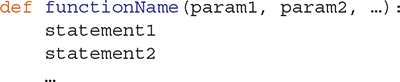
The def statement begins by giving the function a name. Next, we specify any parameters we want our function to accept. In Python, we can have zero or more parameters for any function we write. All the parameters must be listed inside the parentheses that follow the function name. Next, we have a colon character, which tells the Python interpreter that the sequence of indented statements that follow is part of the function. Python knows to stop reading lines for the def statement when it encounters a line that is not indented. A group of Python statements that are indented at the same level are called a block.
Now let’s try to write a real function. Suppose that we are working on a graphics program that requires us to draw a lot of squares. Telling the turtle how to draw a square each time we need one is tiresome and repetitious. In fact, a square is an example of an abstraction. We know that a square is a geometric shape that has four sides of equal length, and four 90-degree corners. What we don’t know is how long the sides are for any particular square.
Our goal is to write a function that can use any turtle to draw a square of any size. To solve this problem, then, we need two pieces of information—namely, the turtle that will draw the square and the size of the square. These pieces of information will become the parameters to our function.
The next step is to use the parameters along with the built-in methods of a turtle. We can draw a square by moving the turtle forward and turning right by 90 degrees four times in a row. LISTING 1.1 shows a complete Python function for drawing a square with a turtle.
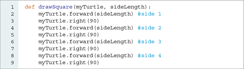
LISTING 1.1 A function to draw a square using a turtle
Notice that the statements in the function are the same turtle commands that we typed in interactively when we first started using the turtle. Placing the commands inside the function groups them together so that we can have the whole set of commands run as if we had typed them one after another. This is one of the great powers of writing a function. It is also important to remember that Python will execute the commands in exactly the order they are typed in the function.
One new element to note in Listing 1.1 is the hash character (#) that appears on lines 2, 4, 6, and 8. This hash character starts a comment. The Python interpreter ignores any text following the hash character until the end of the line. Thus, comments allow the programmer to place descriptive documentation into Python code that will not impact the execution of the program. You will see comments in many of our sessions.
Type the drawSquare function into a text file using Notepad or TextEdit exactly as shown in Listing 1.1, including the indentation of the function block. After you type in the function, save it to a file called ds.py. To make it easy to find this file, set IDLE’s “Start in” property to the folder where you saved the file. You have just created your first module! In the same way that turtle is a module created by other Python programmers, you have created a module called ds.
We can now use the drawSquare function, as shown in SESSION 1.10. After running the commands in this session, you should have an image that looks like FIGURE 1.10.
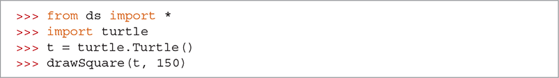
SESSION 1.10 A Python session that demonstrates calling a function
FIGURE 1.10 The result of the statements in Session 1.10.
© 2001–2019 Python Software Foundation; All Rights Reserved.
There is a lot going on in this simple example, but there are only a few new things that you have not seen before. First, we import the turtle and ds modules. When we execute the statement import turtle, any functions inside the turtle module are “hidden” from us unless we use the turtle prefix. However, if we use the statement from ds import *, all the functions defined in the file ds.py are visible to us without the ds prefix.
We then make a new turtle object named t, and next we call drawSquare. Python knows that it should treat the object drawSquare like a function call because of the parentheses that follow its name. You can even prove to yourself that drawSquare is a plain old object by typing drawSquare without the parentheses after the name. If you do so, Python will tell you something like <function drawSquare at 0x000001C3863E01E0>.
When we call the function drawSquare, we pass it two objects, t and 150. When a function is called, the objects are matched up with the parameter names they were given when we defined the function. The first parameter in the list names the first object, the second parameter in the list names the second object, and so on. In this case, t goes by the name myTurtle inside the drawSquare function. The turtle object now has two names. Similarly, inside the drawSquare function, 150 now has the name sideLength.
The reference diagram in FIGURE 1.11 indicates how all the names and objects are matched up. This diagram is simplified somewhat, but we will add more details to such diagrams in later chapters. The important thing to notice is the relationship between the names of the parameters of a function and the objects that are passed to the function when it is called.
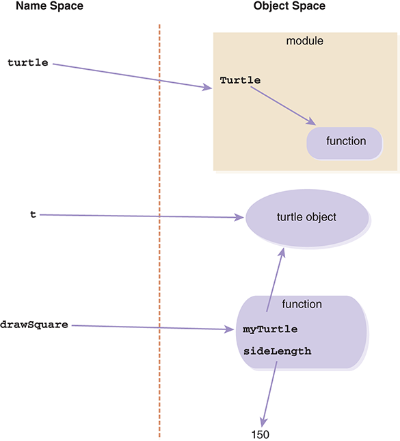
FIGURE 1.11 A reference diagram for the function drawSquare.
Figure 1.11 shows three names: (1) turtle, which references the turtle module we imported previously; (2) t, which references the turtle object we created with the call to the turtle constructor (turtle.Turtle()), shown inside the turtle module; and (3) drawSquare, which references the function object we defined for drawing squares. In the function object named drawSquare, you can see two additional names: (1) myTurtle, which references the turtle object named t, and (2) sideLength, which references the integer object 150 that has no other name.
1.5.4 Repetition
Although the drawSquare function we discussed earlier worked correctly, our solution is unsatisfying in one respect: We had to duplicate the move forward and turn to the right statements four times. We can eliminate this duplication by using a statement that Python provides for repeating a block of code multiple times—a for loop. The for loop is an example of using repetition in our program.
Before we rewrite our drawSquare function, let’s look at the structure of a for loop to get a better idea of how this statement works:
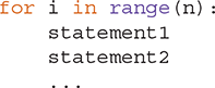
Notice that the for loop template has some similarity to the def template. There is a beginning line ending with a colon, followed by an indented block of code. All you need to know about a for loop at this point is that each statement in the indented block will be evaluated n times, where n is the parameter to the range function. If the first line was for i in range(10):, then each statement would be evaluated 10 times. We will talk more about the range function as well as the i and in parts of the statement shortly.
Now let’s see how we can use this idea of simple repetition to make our drawSquare function more elegant. In fact, all we need to do is wrap the two lines that tell the turtle to move forward and turn right inside a loop that will be evaluated four times. You can see the new and improved drawSquare function in LISTING 1.2.
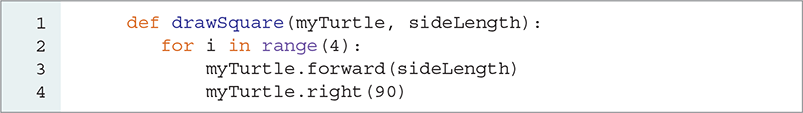
LISTING 1.2 A better version of the drawSquare function
Drawing a Spiral
Our goal for this section is to understand how we can use the for loop to have the turtle create a more complicated square spiral pattern. To create a spiral pattern, the sides of our square need to grow each time the turtle moves forward. We can make that happen easily when we understand the two components of the for statement that we ignored a moment ago.
First, let’s look at the range function. If you ask Python to evaluate the expression range(5), you will get back a sequence object representing the numbers [0, 1, 2, 3, 4].
The range function is very versatile: It can create all kinds of sequences depending on the parameters that we supply. We can call range in three ways:
▶
range(stop): Creates a sequence of numbers beginning at0and going up tostop-1, incrementing by1.▶
range(start, stop): Creates a sequence of numbers beginning atstartand going up tostop-1, incrementing by1.▶
range(start, stop, step): Creates a sequence of numbers beginning atstartand going up tostop-1, incrementing bystep.
Now that you have a better understanding of the range function, let’s look at the loop variable—the variable that always follows the keyword for. In LISTING 1.3, the loop variable is named sideLength. In Python, this loop variable starts with the name for the first item in the sequence produced by the range function the first time through the loop. The second time through the loop, the loop variable is the name for the second item in the sequence, and so on until there are no more items in the sequence. We can use any valid Python name for the loop variable.
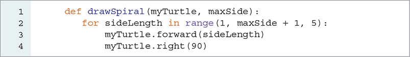
LISTING 1.3 A Python function to draw a spiral
FIGURE 1.12 shows the sequence produced by the call to range and the item in the list named by item during the fourth repetition of the loop. Note that 55 is the last item in the sequence because the upper bound, 60, is not included in the result of the range function.
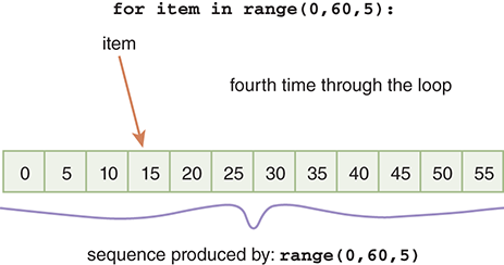
FIGURE 1.12 A loop variable naming each item in a sequence.
Loop variables can be used in expressions and function calls like any other Python names. To solve the spiral problem, Listing 1.3 uses a loop variable in a function named drawSpiral that draws a spiral. The parameters to this function are the turtle and a bound for the longest side on the spiral. We start with the first side having length 1; each time through the loop, we increase the length of the next side of the spiral by 5.
FIGURE 1.13 illustrates the first four iterations of the for loop in Listing 1.3. In the first iteration, the turtle draws a line that is 1 unit long because sideLength refers to the first item in the sequence produced by range(1, maxSide + 1, 5), which is 1. In the second iteration, sideLength refers to the number 6, so the turtle draws a line that is 6 units long. In the third iteration, sideLength refers to 11; in the fourth iteration, sideLength refers to the fourth number in the sequence, which is 16.
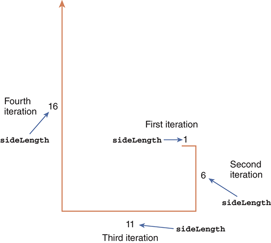
FIGURE 1.13 The first four iterations of the loop in drawSpiral(t, 150).
Drawing a Circle
Our final problem for this chapter is to write a function that uses a turtle to draw a circle of a given radius. Although this may seem like a daunting task, we will help ourselves by solving a simpler problem first and then using what we learn to solve the more general problem. The first challenge is that the turtle’s functionality allows us to draw only straight lines. But by drawing many short straight lines, we can approximate a curved line.
Suppose that our problem was to draw a triangle rather than a circle. Starting from the drawSquare function, it is not too hard to imagine how we would modify drawSquare to write drawTriangle. We would change the call to range(4) to be range(3), as we now need only three sides. We would also change the number of degrees we pass as the parameter for our right turn function.
How many degrees do we need to turn each time to draw an equilateral triangle? When the triangle is complete, we want our turtle to be pointed in the same direction it was when we started. So, as we draw the three sides of our triangle, the turtle will turn through 360 degrees. That matches our drawSquare function, where we made four 90-degree turns (4 × 90 = 360). So, to draw a triangle, we will use 360 ÷ 3 = 120 for our turning angle. LISTING 1.4 shows the small changes made to the drawSquare function to create the drawTriangle function.
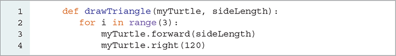
LISTING 1.4 A Python function to draw a triangle
We now have two simple examples of polygons—the equilateral triangle and the square. It is relatively easy to imagine how we would write a function to draw a pentagon or an octagon by following the pattern we have established with the triangle and square. In fact, TABLE 1.7 illustrates the values we would supply to the range and right functions for several different polygons.
TABLE 1.7 Number of Sides and Turning Angle for Several Polygons |
|---|
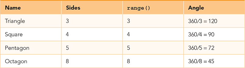
|
Table 1.7 suggests that we can write a function that is more abstract than drawSquare, drawTriangle, or even drawOctagon. The abstraction we are using in this case is a regular polygon. Creating one function that can replace many simpler functions at a higher level of abstraction is a common and important problem-solving technique in computer science.
For example, we can write a function that draws any regular polygon if we pass the function a third parameter. The third parameter tells the function how many sides we want. Once we know how many sides are required, we can easily calculate the turning angle by using the formula turnAngle = 360 / numSides. You can see the new drawPolygon function in LISTING 1.5.
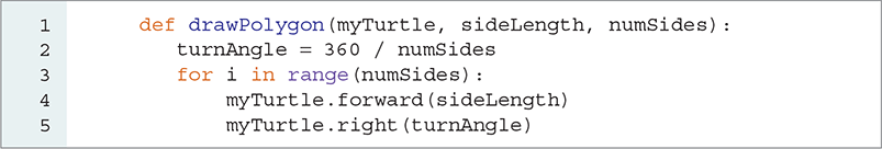
LISTING 1.5 A Python function to draw a regular polygon of any size
SESSION 1.11 and FIGURE 1.14 illustrate several calls to the drawPolygon function, assuming we have saved the code into a file named dp.py. Before we call the drawPolygon function, however, we want to move the turtle to the left and make it face upward. To do so, we lift the turtle’s tail so that the turtle will not leave a path when it moves: We move the turtle backward 200 pixels, turn the turtle 90 degrees to the left, and then put the tail down.
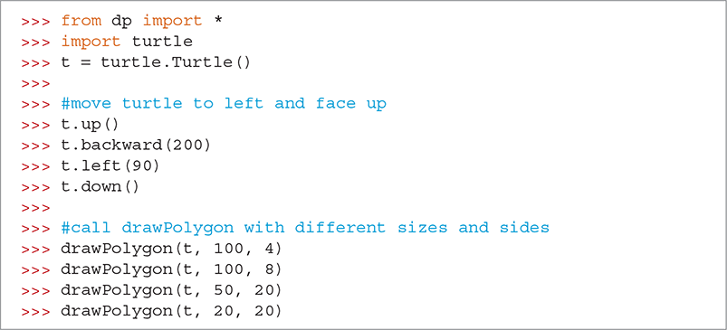
SESSION 1.11 Testing the drawPolygon function
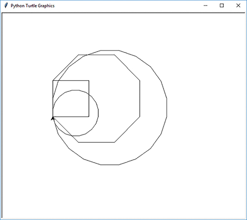
FIGURE 1.14 Several polygons drawn by the drawPolygon function.
© 2001–2019 Python Software Foundation; All Rights Reserved.
Note that the call drawPolygon(t,20,20) makes a pretty good approximation of a circle.
So far, we have worked our way through the problem of drawing a circle by using a large-degree polygon as an approximation. Now let’s return to the original problem statement, which asks us to draw a circle of a given radius. Our last trick is to figure out how to use the radius to compute the number of sides and the side length.
Suppose that to get the smoothest circle possible, even when we are drawing a very large circle, we choose to always have 360 sides to our polygon. With this specification, the turtle will always turn 1 degree and should give us a smooth circle even for a large radius.
Only one question remains: How do we decide what side length to use for a given radius? One good approximation is to use the relationship of the radius of a circle to the circumference. If we are doing a good job of approximating a circle, then the circumference of the circle should be very close to the sum of the individual sides of the polygon. Recall that the circumference of a circle can be calculated from the radius using the formula circumference = 2 × π × radius. Once we have the circumference, we can calculate an individual side length by dividing the circumference by the number of sides, which we have decided will be 360. LISTING 1.6 shows the drawCircle function, which makes use of our drawPolygon function to draw a circle with a given radius.
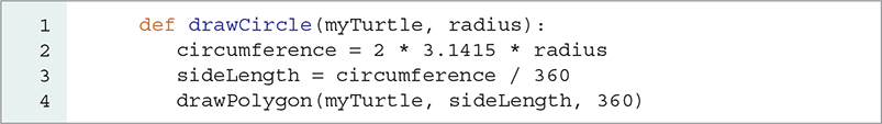
LISTING 1.6 A Python function to draw a circle
The drawCircle function is extremely simple because we have reduced the problem of drawing a circle to that of drawing a polygon with a particular number of sides and side lengths. First, we calculate the circumference; then, we calculate the side length given the circumference and number of sides. Because we already know how to draw a polygon, we do not have to redo that work. We can build on what we have already accomplished and use the drawPolygon function to perform this tedious work. SESSION 1.12 and FIGURE 1.15 illustrate the use of the drawCircle function to draw both a large circle and a small circle. We assume that you have added the drawCircle function to the file dp.py.
SESSION 1.12 Drawing a circle
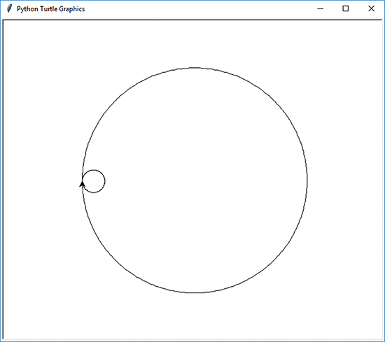
FIGURE 1.15 Drawing a circle for a given radius.
© 2001–2019 Python Software Foundation; All Rights Reserved.