9.4 Snowflakes, Lindenmayer, and Grammars
It is said that no two snowflakes are exactly alike. Snowflakes are another item in nature that can be reproduced by using fractal techniques. The photo in FIGURE 9.7 shows a snowflake. The snowflake in FIGURE 9.8 was produced using the Koch curve, a fractal algorithm developed by Helge von Koch in 1904.
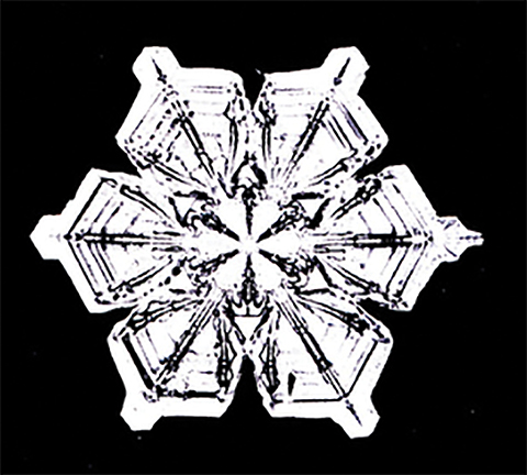
FIGURE 9.7 Photo of a snowflake.
Wilson Bentley. Courtesy of National Oceanic and Atmospheric Administration/Department of Commerce.
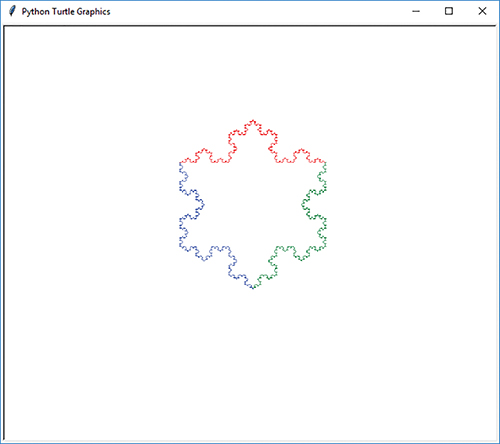
FIGURE 9.8 A snowflake produced using a fractal algorithm developed by Helge von Koch.
© 2001-2019 Python Software Foundation. All Rights Reserved.
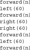
A Koch snowflake is constructed from several Koch curves. Let’s look at Koch’s algorithm for drawing a curve in more detail. The simplest possible curve is actually a straight line of length n, the base case. The next easiest curve can be described in terms of the following set of turtle instructions:
If you think recursively about the curve, you can imagine that each straight line can be replaced by a set of shorter lines following this set of instructions. FIGURE 9.9 illustrates the Koch curve at several levels of detail.
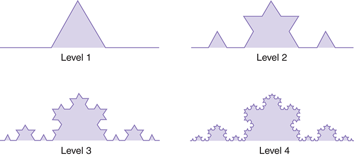
FIGURE 9.9 Four levels of a Koch curve.
At this point you could write a simple recursive function to plot a Koch curve. (In fact, Try It Out exercise 9.23 asks you to do so.) But let’s think a bit differently about fractals and recursion.
9.4.1 L-Systems
The biologist Astrid Lindenmayer invented the L-system in 1968. The L-system is a formal mathematical theory designed to model the growth of biological systems. This construct can be used to specify the rules for all kinds of fractals.
As it turns out, L-systems are based on a formal idea from computer science called a grammar, which may be used for many purposes, including the specification of programming languages. A grammar consists of a set of symbols and one or more production rules. These rules specify how one symbol can be replaced by one or more other symbols. A production rule has two parts:
the left side, which specifies a symbol, and
the right side, which specifies the symbols that can replace the symbol on the left.
Let’s look at a simple example of a grammar:
| Axiom | A |
| Rules (1) | A → B |
| (2) | B → AB |
We can interpret this grammar as follows, beginning with the axiom, the starting point. Axiom A is the simplest string you can produce in the grammar. You may also think of the axiom in terms of a base case for the grammar. The rules tell us how we can construct more complicated strings that are part of the grammar. For example, rule 1 tells us that we can substitute the string B for the string A, and rule 2 tells us that we can change the string B into the string AB.
When you apply the rules to a string, you must work from left to right, applying the rule where the left side matches the current symbol. If a rule matches, then you must apply the rule. Let’s look at an example:
| A | Axiom |
| B | (apply rule 1 to A) |
| AB | (apply rule 2 to B) |
| BAB | (apply rule 1 to A, then apply rule 2 to B) |
| ABBAB | (apply rule 2 to B, then rule 1 to A, then rule 2 to B) |
| BABABBAB | (rules applied: 1, 2, 2, 1, 2) |
Try to apply the rules and produce a few more lines on your own. If you are applying the rules correctly, you will notice that the length of each string follows the Fibonacci sequence of numbers: 1, 1, 2, 3, 5, 8, 13, 21, . . . .
To make the transition from these simple L-systems to an L-system that a turtle can use to draw pictures, consider the interpretation of the symbols used to define the L-system. Suppose that rather than using the symbols A and B, we used the symbols F, B, +, and −.
▶ F indicates that the turtle should move forward and draw a line.
▶ B indicates the turtle should move backward while drawing a line.
▶ The “+” symbol indicates that the turtle should turn right.
▶ The “−” symbol indicates that the turtle should turn left.
Let’s return to the Koch curve and consider the set of steps we outlined to draw a simple curve. We can specify the following set of actions as an L-system:
| Axiom | F |
| Rule | F → F − F + + F − F |
Notice that the axiom gives us a straight line, which is the simplest Koch curve. But if we apply the production rule one time, we get the string F−F++F−F. This gives us the next simplest Koch curve.
Applying the production rule to the string F−F++F−F gives us the following string:

Given a string of instructions, it is straightforward to write a Python function that could interpret the string and make the appropriate calls to turtle methods. To successfully draw a Koch curve, we would need to know the distance to have the turtle go forward, along with the angle for the turtle’s turn.
LISTING 9.6 shows the code for the function drawLS. This function simply iterates over each character in the instruction string. When it encounters an “F” or “B”, the turtle is instructed to move forward or backward distance units. When a “+” or “--” is encountered, the turtle is instructed to turn right or left by angle degrees. If any other character is encountered, the function prints an error message.
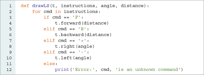
LISTING 9.6 A simple function to follow an L-system string
9.4.2 Automatically Expanding Production Rules
Applying the production rules in an L-system can be tedious, so let’s write a function to automate the process. We first need to determine “how production rules can be represented in Python.” In fact, this problem is similar to the translation problem described in the Introducing the Python Collections chapter. The solution is to use a Python dictionary.
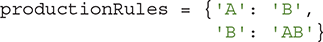
A dictionary can represent any number of production rules, where the left side of the rule is the key and the right side of the rule is the value. For example, the following set of production rules generates the Fibonacci numbers:
| Axiom | A |
| Rules | A → B |
| B → AB |
The Python dictionary that corresponds to these rules can be stored as follows:
Now let’s write a Python function to take an initial string and apply a set of production rules a specified number of times. LISTING 9.7 shows the Python function applyProduction.
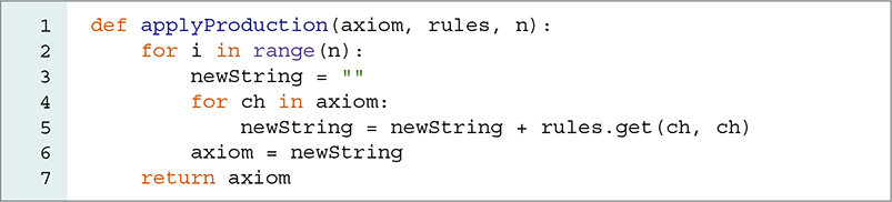
LISTING 9.7 Automatically applying production rules
Everything in the applyProduction function should look familiar. The outer loop allows us to apply the production rules to the string n times. The inner loop is a simple accumulator pattern that allows us to construct a new string by applying the production rules one character at a time. Notice the statement rules.get(ch,ch) shown on line 5. This statement elegantly handles the case in which we encounter a character but do not have a production rule for expanding the character further. Recall that the get method allows us to specify a default value for the case that a key is not found in the dictionary. In this instance, when character ch has no production rule, we simply leave the character in place.
SESSION 9.3 shows the applyProduction function in action using the Fibonacci production rules.
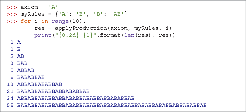
SESSION 9.3 Using the production rule expander
9.4.3 More Advanced L-Systems
To use L-systems to model plant growth, we need to add one more features to our grammar: the characters "[" and "]". The left square bracket and right square bracket characters represent operations to save and restore the state of the turtle. Whenever the function encounters a "[" in the string, the position and heading of the turtle are saved. When it encounters a "]", the position and heading from the last save are restored.
Using these new characters, we can now use an L-system to specify the tree we drew using Listing 9.4. The grammar for this new L-system is as follows:
| Axiom | X |
| Rules | X → F[−X]+X |
| F → FF |
Starting with the axiom X and applying the production rules twice gives us the following string:

Suppose that we use an angle of 60 degrees and a distance of 20 units. This string instructs the turtle to take the following actions:
Go forward a total of 40 units.
Save the position and heading; call this state W.
Turn left 60 degrees.
Go forward 20 units.
Save the position and heading; call this state Z.
Turn left 60 degrees.
Do nothing. X is not a recognized turtle command.
Restore the turtle position from the saved state called Z.
Turn right 60 degrees.
Do nothing.
Restore the position and heading from the saved state called W.
Turn right 60 degrees.
Go forward 20 units.
At this point, we have succeeded in drawing a Y. But notice the difference between this approach and the code in Listing 9.4: We no longer need to have the turtle back up. By using the save and restore operations, we can simply jump the turtle back to any previous position.
Let’s modify the drawLS function to support the save and restore operations. LISTING 9.8 shows the new function. In this version, we have removed the final else statement with the corresponding error message: This allows the function to silently ignore any commands it does not recognize. The stateSaver list allows us to append new states that we want to save to the end of the list. Using the pop method, we can restore the most recently saved state.
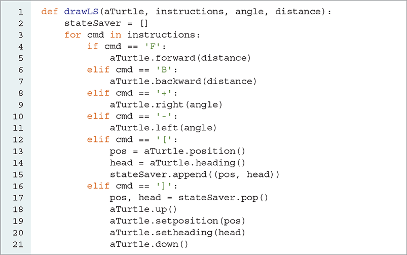
LISTING 9.8 An improved L-system drawing function
Finally, let’s write a simple function that combines all our work into a single function that applies the production rules and draws the resulting L-system. The lSystem function takes seven parameters:
axiom |
The initial axiom |
rules |
A dictionary specifying the production rules |
depth |
The number of times to expand the production rules |
initialPosition |
The initial position for the turtle |
heading |
The initial heading for the turtle |
angle |
The angle to turn for the “+” and “−” operations |
length |
The distance to move forward or backward for an “F” or “B,” respectively |
The code for the lSystem function is shown in LISTING 9.9. In SESSION 9.4, we use this function to draw a simple tree.
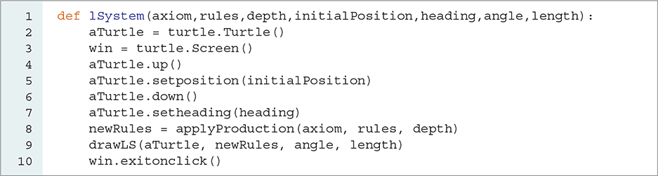
LISTING 9.9 A function to expand and draw an L-system
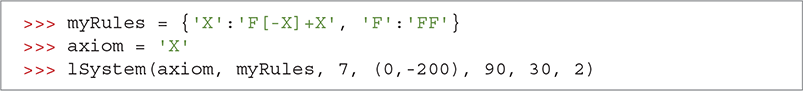
SESSION 9.4 Drawing a tree using an L-system
Here are the rules for drawing something that looks like a sprig of rosemary:
| Axiom | H |
| Rules | H → HFX[+H][ − H] |
| X → X[ − FFF][+FFF]FX |
Using a level of 5, an angle of 25.7 degrees, and a length of 8, we get the image shown in FIGURE 9.10. We also modified lSystem to set the color. In this case, we used 'darkgreen'.
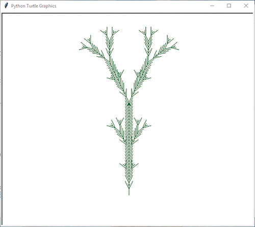
FIGURE 9.10 A sprig of rosemary drawn by a turtle.
© 2001–2019 Python Software Foundation. All Rights Reserved.
From here on, you are on your own to explore the world of L-systems. The following exercises have some examples to get you started, but you can find many more by doing some research.