9.3 Recursive Programs
Before we look at the program used to draw the tree, we must first learn a little more about recursion. In computer science and mathematics, a recursive function is a function that calls itself. A very simple, but erroneous, illustration of a recursive function is shown in LISTING 9.1.

LISTING 9.1 An erroneous recursive function
The hello function prints the message "Hello World" and then calls itself again. If you ran this function in Python, the program would continue to call itself and print "Hello World" until Python simply crashed. Clearly, there’s more to a successful recursive function than simply calling itself.
A more useful way of thinking about recursive functions is as follows:
Are we done yet? Have we found a problem that is small enough to solve trivially? If so, solve it without any further work and return the answer.
If not, simplify the problem, and solve the simpler problem. Combine the result of solving the simplified problem with what you know to solve the original. Return the combined result.
The first step is called the base case. Every recursive program must have a base case so that it knows when to stop. Checking for the base case is what’s missing from the program in Listing 9.1.
The second step is often called the recursive step. The recursive step involves simplifying the problem in a way that moves it closer to the base case. Sometimes you will need to combine the result returned by the recursive call with some data you saved when you simplified the problem. In other cases, the problem is solved just by making the simplifying step.
9.3.1 Recursive Squares
Let’s look at a problem of drawing the nested boxes shown in FIGURE 9.2.
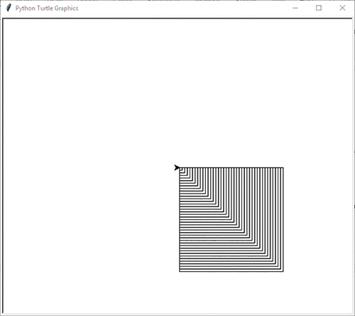
FIGURE 9.2 Nested boxes.
© 2001–2019 Python Software Foundation. All Rights Reserved.
In this case, we need to draw a series of squares. We know how to draw a single square, but how do we draw the entire picture? Let’s start by identifying the base case. Since drawing a square that has a side length of 1 unit is the smallest possible square, we will identify the base case as the side length being less than 1. The simplification step is to recursively draw smaller and smaller squares as long as the side length is greater than or equal to 1.
LISTING 9.2 shows the code for the nested boxes. The drawSquare function should look familiar to you: It simply draws a square of a specified size. The nestedBox function is a recursive process that follows the two important steps outlined previously. First, line 7 checks for the base case. The expression side >= 1 will evaluate to False as soon as the side parameter is less than 1. Because there is no else clause, notice that as soon as the base case is reached (side is less than 1), the nestedBox simply returns without doing anything.
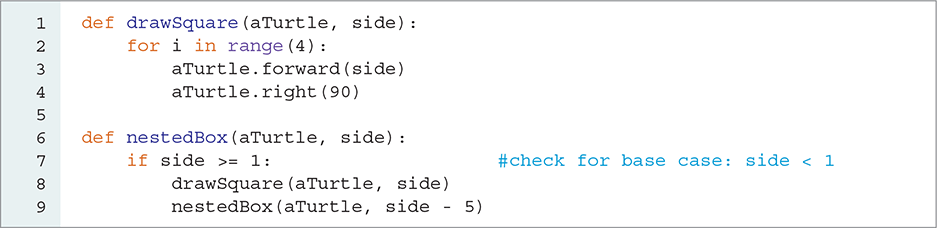
LISTING 9.2 Recursively drawing boxes
If the value of side is greater than or equal to 1, we draw a square that has a length of side. After the square is drawn, the next step is to call nestedBox recursively, reducing the side length by 5. By reducing the value of side by 5, we are moving toward the base case.
9.3.2 Classic Recursive Functions
It is also often possible to use recursion to express mathematical functions in an elegant way. The following exercises allow you to explore simple recursion by writing some nongraphical functions. The key to handling lists recursively is to process one item from the list and then call the method again with that item removed from the list, continuing this pattern until the parameter list is empty or contains only one item, depending on the problem. The approach for strings is similar.
For example, LISTING 9.3 shows a recursive function that counts the number of items in a list. The base case occurs when the list is empty. If the list is not empty, then we count the first item (add 1), and recursively call the method with the remaining items in the list.
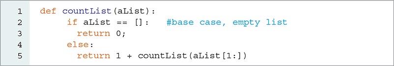
LISTING 9.3 Recursively counting items
9.3.3 Drawing a Recursive Tree
Let’s return to the problem of drawing the tree in Figure 9.1. Recall the instructions for drawing the tree:
Draw a trunk that is n units long.
Turn to the right 30 degrees, and draw another tree with a trunk that is n − 15 units long.
Turn to the left 60 degrees, and draw another tree with a trunk that is n − 15 units long.
Now let’s apply the rules for recursion to implement a program that follows the tree-drawing instructions.
First, we must identify the base case. When drawing a tree, the base case is a tree where the trunk length is less than some predefined value. We could say that a trunk length of 1 is the smallest possible tree we could draw, but in fact we can pick any number to use as the smallest trunk length. If the trunk length is less than or equal to our predefined minimum, we simply stop drawing new trees and return.
We have already seen the recursive step in drawing the tree—actually, there are two recursive steps. Steps 2 and 3 both specify that we need to “draw another tree.” Notice that not only are we drawing another tree (recursively), but we are also making progress toward the base case by drawing a trunk that is smaller than the current trunk length. LISTING 9.4 shows our recursive Python function that takes a turtle and a starting trunk length.
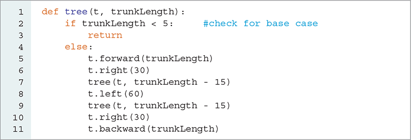
LISTING 9.4 A recursive tree function
The amazing thing about the tree function is its length—only 11 lines. Recursion often offers us the capability of elegantly capturing a complex process. Let’s look at the code in Listing 9.4 carefully and see how it compares with the rules we defined. First, notice that we check for the base case on line 2. We have written the program to be slightly longer than is strictly necessary to make it clear that we are checking for the base case. We could remove the explicit return and the else clause if we changed the conditional to trunkLength >= 5.
If we have not reached the base case, the turtle moves forward and turns to the right 30 degrees. On line 7, we make the first recursive call to draw a smaller tree on the right side of the trunk. When this side of the trunk is done, then the function returns and turns 60 degrees to the left, and the left side of the trunk is drawn. Run this program and carefully watch the order in which the branches are drawn.
SESSION 9.1 shows the preparation and function call. Notice that the turtle needs to be moved to the lower part of the window and turned 90 degrees to the left before making the initial call to the function because we want the tree to grow up. After the tree has been drawn, we hide the turtle.
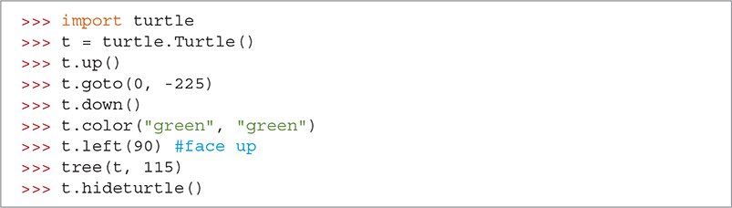
SESSION 9.1 Calling the recursive tree function
9.3.4 The Sierpinski Triangle
Let’s look at another simple fractal called the Sierpinski triangle. Imagine that you have three triangles that are all the same size. If you take the first two triangles, put them side by side, and then balance the third triangle on the peaks of the first two triangles, you will get a new, larger triangle composed of those three triangles. Further suppose that you constructed each of the three original triangles from three smaller triangles, and each of the three smaller triangles with three smaller triangles still. FIGURE 9.3 gives you an idea about what is involved. The idea of self-similarity at increasingly smaller scales is key to the concept of a fractal, and it is key to understanding recursion.
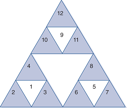
FIGURE 9.3 The Sierpinski triangle.
Writing a program to draw the Sierpinski triangle is more complex than writing a program to draw a fractal tree, but it is still surprisingly simple. We will use the depth, which represents the number of times we subdivide the original triangle, as the movement toward the base case. When we reach a sufficient depth, we will then draw a triangle of the appropriate size for that depth. In fact, we start the depth with a positive number, and each time we recursively divide a triangle, we subtract 1 from the depth. When we reach a depth of zero, we finally draw a very small triangle.
The Sierpinski triangle shown in Figure 9.3 has a depth of 2. Notice that there are nine shaded triangles, which represent the triangles drawn by the base case. The triangles numbered 1, 5, and 9 were not drawn but are artifacts of the three surrounding triangles. FIGURE 9.4 shows a Sierpinski triangle of depth 5.
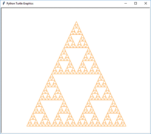
FIGURE 9.4 A Sierpinski triangle of depth 5.
© 2001–2019 Python Software Foundation. All Rights Reserved.
The sierpinski function will accept three points as parameters; these points define the three corners of the triangle. To subdivide a large triangle into three smaller triangles, we use the following rule:
For each corner of the large triangle, create a small triangle using the given corner and the points that are halfway between the given corner and the other two corners.
For example, consider triangle ABC in FIGURE 9.5. The three new triangles we can construct are triangles A-1-3, B-2-1, and C-3-2.
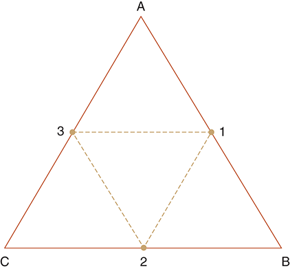
FIGURE 9.5 Splitting a triangle equally.
To calculate points 1, 2, and 3, we find the midpoints of the line segments AB, BC, and CA, respectively. Recall that we can calculate the midpoint of a line segment (mx, m y) by using the equations
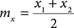
and
Drawing the smaller triangles is the recursive step in our function. It will involve three recursive calls to the sierpinski function using the vertices calculated by the method just described.
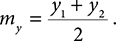
The function we will write requires two simple helper functions: a function to draw a triangle and a function to calculate the coordinates of a point halfway between two other points. The drawTriangle function takes a turtle and three points as parameters. The goto method is used to connect the three points. The midPoint function encodes the equation for the midpoint of the segment and returns a tuple giving the x and y coordinates of the midpoint.
The sierpinski function and the two helper functions are shown in LISTING 9.5. Note that the final version of the function has a parameter for the turtle as well as a parameter for the depth. The first line of sierpinski checks whether the depth is greater than zero. If that is the case, we make three recursive calls to sierpinski. Each recursive call represents one of the three subtriangles. When we make the recursive call, we subtract 1 from the depth to move toward the base case. When the function reaches a depth of zero, no more recursion is required. At this point, a triangle is drawn and the function simply returns. The larger the depth specified originally, the smaller this triangle will be.
LISTING 9.5 Drawing a Sierpinski triangle
SESSION 9.2 shows the code used to create the Sierpinski triangle in Figure 9.4. As noted earlier, the depth of that triangle is 5.
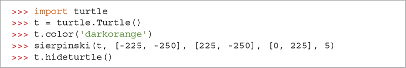
SESSION 9.2 Creating the Sierpinski triangle
9.3.5 Call Tree for a Sierpinski Triangle
By now, you have probably tried to run the sierpinski function on your own a few times, and it should now be clear that the triangle is drawn in thirds. After one-third of the larger triangle has been completed, then the next third is drawn, and finally the last third is drawn. Within each smaller third, the same behavior holds true.
We can graph this behavior using a call tree, which enables us to order the recursive calls to the sierpinski function to explain why the triangle is drawn using this sequence. The call tree for a Sierpinski triangle of depth 2 is shown in FIGURE 9.6. Notice that the labels on the arrows on the call tree match the triangle numbers shown in Figure 9.3.
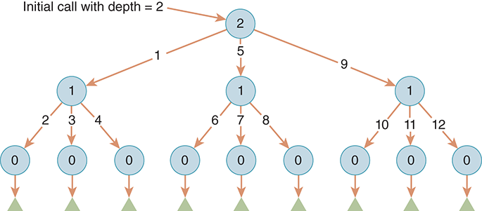
FIGURE 9.6 The call tree for a Sierpinski triangle of depth 2.