
Origin of renewable energy flows
Abstract
The basic physical processes responsible for availability of renewable energy sources on Earth are described, from formation of and properties of solar radiation, over processes taking place near the surface of the Earth (in atmosphere, hydrosphere, and lithosphere) to comprehensive models attempting to capture enough of the determinants for circulation and climate to be able to understand present and future climates.
Keywords
Solar radiation; Energy production in stars; Disposition of radiation at the surface of the Earth; Energy and matter cycles of the Earth; Meteorological models; Climate models; Scales of atmospheric motion
In this chapter, renewable energy is followed from the sources where it is created—notably the Sun—to the Earth, where it is converted into different forms, e.g., solar radiation to wind or wave energy, and distributed over the Earth–atmosphere system through a number of complex processes. Essential for these processes are the mechanisms for general circulation in the atmosphere and the oceans. The same mechanisms play a role in distributing pollutants released to the environment, whether from energy-related activities like burning fossil fuels or from other human activities. Because the assessment of environmental impacts plays an essential part in motivating societies to introduce renewable energy, the human interference with climate is also dealt with in this chapter, where it fits naturally.
2.1 Solar radiation
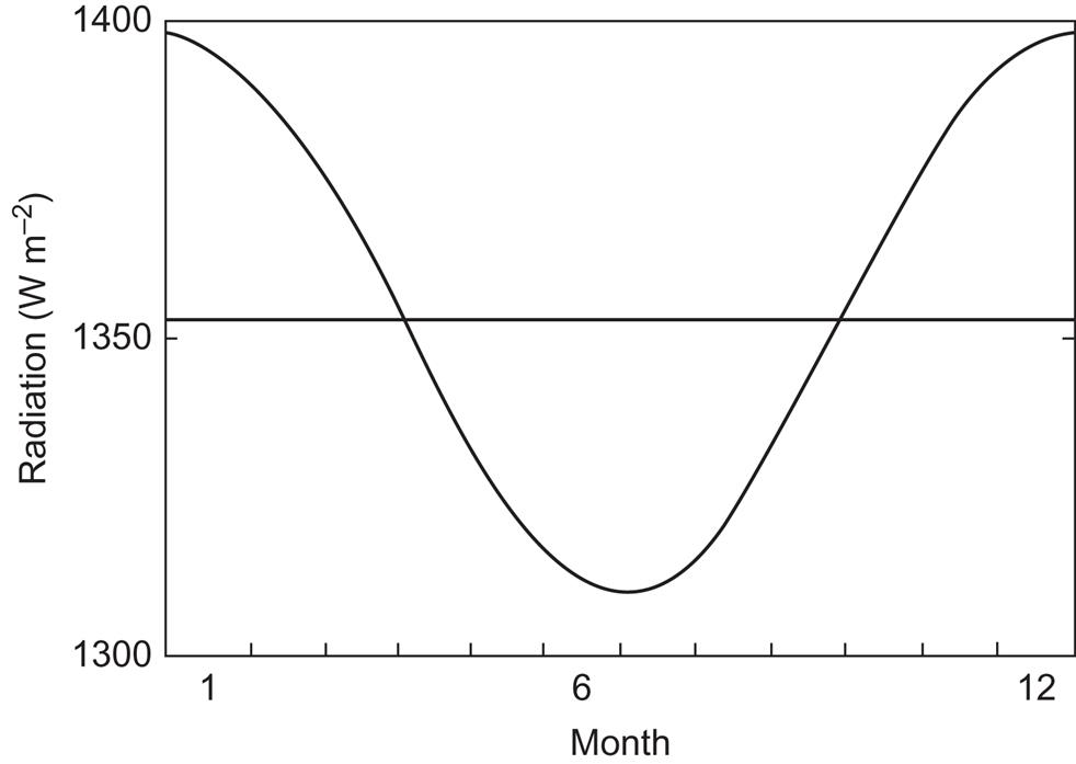
At present the Sun radiates energy at the rate of 3.9×1026 W. At the top of the Earth’s atmosphere an average power of 1353 W m−2 is passing through a plane perpendicular to the direction of the Sun. As shown in Fig. 2.1, regular oscillations around this figure are produced by the changes in the Earth–Sun distance, as the Earth progresses in its elliptical orbit around the Sun. The average distance is 1.5×10¹¹ m and the variation is ±1.7%. Further variation in the amount of solar radiation received at the top of the atmosphere is caused by slight irregularities in the solar surface, in combination with the Sun’s rotation (about one revolution per month), and by possible time variations in the surface luminosity of the Sun.
2.1.1 Energy production in main-sequence stars like the Sun
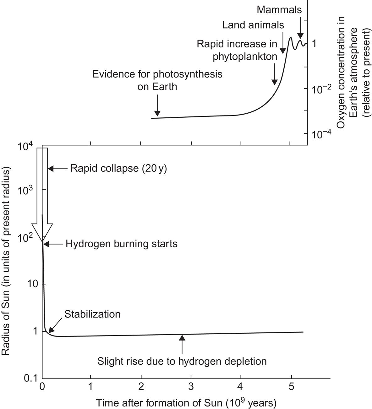
The energy produced by nuclear reactions in the interior of the Sun must equal the amount of energy radiated from the surface, since otherwise the Sun could not have been structurally stable over long periods of time. Evidence for the stability of the Sun comes from several sources. Stability over a period of nearly 3×10⁹ years is implied by the relative stability of the temperature at the Earth’s surface (oxidized sediments and fossil remains indicate that water in its fluid phase has been present throughout such periods). Stability over an even longer time is implicit in our understanding of the evolution of the Sun and other similar stars. As an indication of this stability, Fig. 2.2 shows the variations in the radius of the Sun believed to have taken place since its assumed formation from clouds of dust and gas.
The conversion of energy contained in the atomic constituents of main-sequence stars like the Sun, from heat of nuclear reactions (which transform hydrogen into helium) to radiation escaping from the surface, is largely understood. The basis for regarding such radiation as a renewable source is that it may continue essentially unaltered for billions of years. Yet there is also a possibility of tiny variations in solar energy production that may have profound implications for life on the planets encircling the Sun.
2.1.1.1 The birth and main-sequence stage of a star
Stars are believed to have been created from particulate matter present in a forming galaxy. Contraction of matter is achieved by gravitational processes involving clouds of dust and gas, but counteracted by the increasing pressure of the gases as they are heated during contraction (cf. the equilibrium equations given below). However, once the temperature is high enough to break up molecules and ionize atoms, the gravitational contraction can go on without increase of pressure, and the star experiences a “free fall” gravitational collapse. If this is considered to be the birth of the star, the development in the following period consists of establishing a temperature gradient between the center and the surface of the star.
While the temperature is still relatively low, transport of energy between the interior and the surface presumably takes place mainly through convection of hot gases (Hayashi, 1966). This leads to a fairly constant surface temperature, while the temperature in the interior rises as the star further contracts, until a temperature of about 107 K is reached. At this point the nuclear fusion processes start, based on a thermonuclear reaction in which the net result is an energy generation of about 25 MeV (1 MeV=1.6×10⁻¹³ J) for each four hydrogen nuclei (protons) undergoing the chain of transformations resulting in the formation of a helium nucleus, two positrons and two neutrinos,
After a while, the temperature and pressure gradients have built up in such a way that the gravitational forces are balanced at every point and the gravitational contraction has stopped. The time needed to reach equilibrium depends on the total mass. For the Sun it is believed to have been about 5×10⁷ years (Herbig, 1967). Since then, the equilibrium has been practically stable, exhibiting smooth changes due to hydrogen burning, such as the one shown in Fig. 2.2 for the radius.
2.1.1.2 Nuclear reactions in the Sun
Most of the nuclear reactions responsible for energy production in the Sun involve two colliding particles and two, possibly three, “ejectiles” (outgoing particles). For example, one may write
where Q is the energy release measured in the center-of-mass co-ordinate system (called the “Q-value” of the reaction). Energy carried by neutrinos will not be included in Q. The main processes in the solar energy cycle are
It is highly probable (estimated at 91% for the present Sun) that the next step in the hydrogen-burning process is
Branch 1:
This process requires the two initial ones given above to have taken place twice. The average total energy liberated is 26.2 MeV. In an estimated 9% of cases (Bahcall, 1969), the last step is replaced by processes involving 4He already present or formed by the processes of branch 1,
The following steps may be either
Branch 2:
or, with an estimated frequency among all the hydrogen-burning processes of 0.1%,
Branch 3:
followed by the decay processes
The average Q-values for processes involving neutrino emission are quoted from Reeves (1965). The initial pp-reaction (![]() = hydrogen nucleus = p = proton) receives competition from the three-body reaction
= hydrogen nucleus = p = proton) receives competition from the three-body reaction
However, under solar conditions, only 1 in 400 reactions of the pp-type proceeds in this way (Bahcall, 1969).
In order to calculate the rates of energy production in the Sun, the cross-sections of each of the reactions involved must be known. The cross-section is the probability for the reaction to occur under given initial conditions, such as a specification of the velocities or momenta.
Among the above-mentioned reactions, those that do not involve electrons or positrons are governed by the characteristics of collisions between atomic nuclei. These characteristics are the action of a Coulomb repulsion of long range, as the nuclei approach each other, and a more complicated nuclear interaction of short range, if the nuclei succeed in penetrating their mutual Coulomb barrier. The effective height of the Coulomb barrier increases if the angular momentum of the relative motion is not zero, according to the quantum mechanical description. The height of the Coulomb barrier for zero relative (orbital) angular momentum may be estimated as
where the radius of one of the nuclei has been inserted in the denominator (Ai is the mass of the nucleus in units of the nucleon mass; Zi is the nuclear charge in units of the elementary charge e, and e2/4πε0 = 1.44×10⁻¹⁵ MeV m). Thus, the thermal energy even in the center of the Sun, T(0)=1.5×10⁷ K,
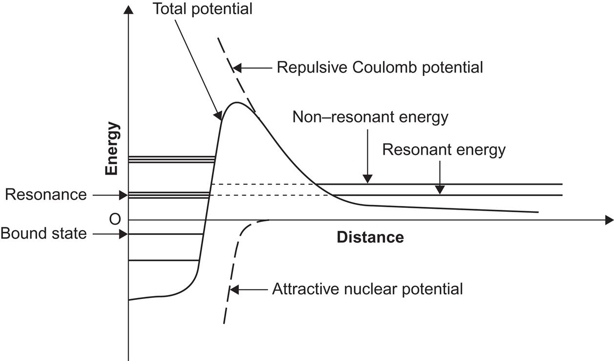
is far below the height of the Coulomb barrier (1 MeV=1.6×10⁻¹³ J), and the nuclear reaction rate will depend strongly on the barrier penetration, i.e., the quantum tunneling through the barrier. If the energy of the approaching particle does not correspond to a nuclear resonance (see Fig. 2.3), then the part of the cross-section due to barrier penetration (and this will contain most of the energy dependence) can be estimated by a simple quantum approximation, called the WKB method (Merzbacker, 1970). In the absence of relative angular momentum, the nuclear reaction cross-section may then be written, as a function of energy,
where S(E) is a slowly varying function of E, depending on the nuclear interactions, while the exponential function expresses the barrier penetration factor in terms of the Coulomb parameter
with the reduced mass being
The reactions involving electrons are governed not by nuclear (so-called “strong”) interactions, but by the “weak” interaction type, which is available to all kinds of particles. The smallness of such interactions permits the use of a perturbational treatment, for which the cross-section may be written (Merzbacker, 1970)
Here vσ is the transition probability, i.e., the probability that a reaction will occur, per unit time and volume. If the formation of the positron–neutrino, electron–antineutrino or generally lepton–antilepton pair is not the result of a decay but of a collision process, then the transition probability may be split into a reaction cross-section σ times the relative velocity, v, of the colliding particles [for example, the two protons in the 1H(1H, e+v)2H reaction]. ρ (final) is the density of final states, defined as the integral over the distribution of momenta of the outgoing particles. When there are three particles in the final state, this will constitute a function of an undetermined energy, e.g., the neutrino energy. Finally, <H> is a matrix element, i.e., an integral over the quantum wavefunctions of all the particles in the initial and final states, with the interaction operator in the middle and usually approximated by a constant for weak interaction processes.
The reaction rate for a reaction involving two particles in the initial state is the product of the numbers n1 and n2 of particles 1 and 2, respectively, each per unit volume, times the probability that two such particles will interact to form the specified final products. This last factor is just the product of the relative velocity and the reaction cross-section. Since the relative velocity of particles somewhere in the Sun is given by the statistical distribution corresponding to the temperature, the local reaction probability may be obtained by averaging over the velocity distribution. For a non-relativistic gas, the relative kinetic energy is related to the velocity by E=1/2μv2, and the velocity distribution may be replaced by the Maxwell–Boltzmann distribution law for kinetic energies (which further assumes that the gas is non-degenerate, i.e., that kT is not small compared with the thermodynamic chemical potential, a condition that is fulfilled for the electrons and nuclei present in the Sun),
The reaction rate (number of reactions per unit time and unit volume) becomes
where δ12 (=1 if the suffixes 1 and 2 are identical, otherwise 0) prevents double counting in case projectile and “target” particles are identical.
The number densities n (number per unit volume) may be re-expressed in terms of the local density ρ(r) and the mass fraction of the ith component, X (e.g., the hydrogen fraction X considered earlier),
The central part of the reaction rate, <σv>, is shown in Fig. 2.4 for the branch 1 reactions of the pp-cycle, as well as for the 3He+4He reaction opening the alternative branches. The basic cross-sections S(0) used in the calculations are quoted in the work of Barnes (1971). The barrier penetration effects are calculated in a modified form, taking account of the partial screening of the nuclear Coulomb field by the presence of electrons. Such penetration factors are included for the weak interaction processes as well as for the reactions caused by nuclear forces.
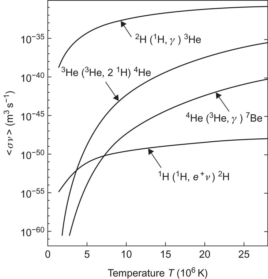
One notes the smallness of the initial, weak interaction reaction rate, the temperature dependence of which determines the overall reaction rate above T=3×10⁶ K. The four to five orders of magnitude difference in the rates of the 4He+3He and the 3He+3He processes account for the observed ratio of branch 2 (and 3) to branch 1, when the oppositely acting ratio of the 4He to 3He number densities is also included.
The rate of energy production to be entered in equation (2.7) below for thermal equilibrium is obtained from the reaction rate by multiplying with the energy release, i.e., the Q-value. Since the energy production rate appearing in (2.7) is per unit mass and not volume, a further division by ρ is necessary,
(2.1)
The sum over j extends over all the different branches; Q(j) is the energy released in branch j; and the indices 1 and 2, for which n1 and n2 are taken and <σv> evaluated, may be any isolated reaction in the chain, since the equilibrium assumption implies that the number densities have adjusted themselves to the differences in reaction cross-section. For decay processes, the reaction rate has to be replaced by the decay probability, in the manner described above.
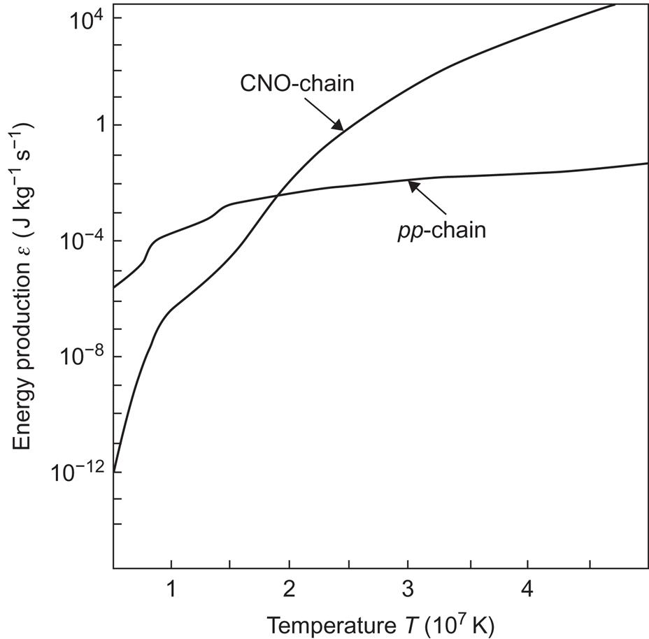
Figure 2.5 shows the temperature dependence of the energy production rate for the pp-chain described above, as well as for the competing CNO-chain, which may come into play at temperatures slightly higher than those prevailing in the Sun’s interior. The curves should be regarded as typical for stars of composition similar to that of the Sun, but as (2.1) indicates, the energy production depends on the density as well as on the abundance of the reacting substances. Hence a change in composition or in central density will change the rate of energy production. For the pp-chain, Fig. 2.5 assumes a hydrogen fraction X=0.5 and a density of 105 kg m−3, believed to be reasonable for the center of the Sun. For the CNO-chain, additional assumptions have been made that the carbon, nitrogen, and oxygen abundances are XC=0.003, XN=0.001, and XO=0.012 (Iben, 1972). These figures apply to stellar populations similar to, but more advanced than, the Sun, whereas much smaller CNO-abundances and production rates are found for the so-called population-II stars. It should also be mentioned that, owing to the decrease in density and change in composition as one goes away from the center of the star, the average energy production for the energy-producing region will be lower than the value deduced from the conditions near the center.
2.1.1.3 Equilibrium processes in the Sun
The present near-equilibrium state of the Sun may be described by a number of physical conditions. The first one is the condition of hydrostatic equilibrium, which states that the pressure gradient at every place must exactly balance the gravitational force. Assuming the Sun to be spherically symmetric, the condition may be written
(2.2)
where M(r) is the integrated mass within a sphere of radius r, ρ(r) is the local density, and G=6.67×10⁻¹¹ m3 kg−1 s−2 is the constant of gravitation.
The pressure P(r) may be related to the local temperature T(r) by an equation of state. The conditions everywhere in the Sun are close to those of an ideal gas, implying
where n(r) is the number of free particles per unit volume and k=1.38×10⁻²³ J K−1 is the Boltzmann constant. Alternatively, one may express n in terms of the gas constant, ![]() = 8.315 J K−1 mol−1, the density, and μ, the mean molecular weight (i.e., the mass per mole of free particles),
= 8.315 J K−1 mol−1, the density, and μ, the mean molecular weight (i.e., the mass per mole of free particles),
For stars other than the Sun the ideal gas law may not be valid, as a result of electrostatic interactions among the charges (depending on the degree of ionization, i.e., the number of free electrons and other “unsaturated” charges) and radiation pressure.
Cox and Giuli (1968) estimate the maximum pressure corrections to be 1.5% from the electrostatic interactions and 0.3% from the radiation pressure, calculated from the blackbody radiation in the Sun’s center. The mean molecular weight may be obtained from assuming the Sun to consist of hydrogen and helium in mass fractions X and (1−X). If all hydrogen and helium is fully ionized, the number of free particles is 2X+3(1−X)/4 and the mass per mole of free particles is
where NA=6×10²³ is Avogadro’s number (the number of particles per mole) and 1.67×10⁻²⁷ kg is the proton mass. The Sun’s hydrogen fraction X is about 0.7.
The potential energy of a unit volume at the distance r from the Sun’s center, under influence of the gravitational forces, is
while the kinetic energy of the motion in such a unit volume, according to statistical mechanics, is
Since εpot is a homologous function of order –1, the virial theorem of classical mechanics (see, for example, Landau and Lifshitz, 1960) states that for the system as a whole,
The bars refer to time averages, and it is assumed that the motion takes place in a finite region of space. Inserting the expressions found above, using R=kNA and integrating over the entire Sun and approximating ∫(M(r)/r)dM(r) by M/R (M and R being the total mass and radius), one finds an expression for the average temperature,
An estimate for the average temperature of the Sun may be obtained by inserting the solar radius R=7×10⁸ m and the solar mass M=2×1030 kg, leading to
The rigorousness of the hydrostatic equilibrium may be demonstrated by assuming a 1% deviation from equilibrium, implying an inward acceleration
The time needed for a 10% contraction (Δr/R=−0.1) under the influence of this acceleration is
at the solar surface R=7×10⁸ m. The observed stability of the solar radius (see Fig. 2.2) demands a very strict fulfillment of the hydrostatic equilibrium condition throughout the Sun.
2.1.1.4 The energy transport equations
In order to derive the radial variation of the density and the temperature, energy transport processes have to be considered. Energy is generated by the nuclear processes in the interior. The part of the energy from nuclear processes that is carried by neutrinos would escape from a star of the Sun’s assumed composition. One may express this in terms of the mean free path of neutrinos in solar matter (the mean free path being large compared with the Sun’s radius) or in terms of the mass absorption coefficient,
with this quantity being very small for neutrinos in the Sun. I denotes the energy flux per unit solid angle in the direction ds, and s denotes the path length in the matter. The alternative way of writing the mass absorption coefficient involves the cross-sections σi per volume of matter of all the absorption or other processes that may attenuate the energy flux.
The energy not produced in association with neutrinos is in the form of electromagnetic radiation (γ-rays) or kinetic energy of the particles involved in the nuclear reactions. Most of the kinetic energy is carried by electrons or positrons. The positrons annihilate with electrons and release the energy as electromagnetic radiation, and also part of the electron kinetic energy is gradually transformed into radiation by a number of processes. However, the electromagnetic radiation also reacts with the matter, notably the electrons, and thereby converts part of the energy to kinetic energy again. If the distribution of particle velocities locally corresponds to that predicted by statistical mechanics (e.g., the Maxwell–Boltzmann distribution), one says that the system is in local thermodynamic or statistical equilibrium.
Assuming that thermodynamic equilibrium exists locally, at least when averaged over suitable time intervals, the temperature is well-defined, and the radiation field must satisfy Planck’s law,
(2.3)
Here F is the power radiated per unit area and into a unit of solid angle, ν is the frequency of radiation, h=6.6×10⁻³⁴ J s is Planck’s constant, and c=3×10⁸ m s−1 is the velocity of electromagnetic radiation (light) in vacuum.
The appropriateness of the assumption of local thermodynamic equilibrium throughout the Sun’s interior is ensured by the shortness of the mean free path of photons present in the Sun, as compared to the Sun’s radius (numerically the ratio is about 10−13, somewhat depending on the frequency of the photons). The mean free path, l, is related to the mass absorption coefficient by
This relation as well as the relation between l and the cross-sections of individual processes may be taken to apply to a specific frequency ν. κ is sometimes referred to as the opacity of the solar matter.
The radiative transfer process may now be described by an equation of transfer, stating that the change in energy flux along an infinitesimal path in the direction of the radiation equals the difference between emission and absorption of radiation along that path,
Integrated over frequencies and solid angles, this difference equals, in conditions of energy balance, the net rate of local energy production per unit mass. In complete thermodynamic equilibrium one would have Kirchhoff’s law, e(ν)=κ(ν)I(ν) (see, for example, Cox and Giuli, 1968), but under local thermodynamic equilibrium, e(ν) contains both true emission and also radiation scattered into the region considered. According to Cox and Giuli (1968), neglecting refraction in the medium,
Here κt and κs are the true absorption and scattering parts of the mass absorption coefficient, and Iav is I averaged over solid angles. Cox and Giuli solve the equation of transfer by expressing I(ν) as a Taylor series expansion of e(ν) around a given optical depth (a parameter related to κ and to the distance r from the Sun’s center or a suitable path length s). Retaining only the first terms, one obtains, in regions of the Sun where all energy transport is radiative,
θ is the angle between the direction of the energy flux I(ν) and ds. The first term dominates in the central region of the Sun, but gives no net energy transport through a unit area. If the path s is taken as the radial distance from the center, the net outward flux obtained by integrating I(ν) cosθ over all solid angles becomes
The luminosity L(r) of a shell of radius r is defined as the net rate of energy flow outward through a sphere of radius r, i.e., 4πr2 times the net outward flux. Introducing at the same time the temperature gradient, one obtains
for the spectral luminosity and
(2.4)
for the total luminosity.
Here σ=5.7×10⁻⁸ W m−2 K−4 is Stefan’s constant in Stefan–Boltzmann’s law for the total power radiated into the half-sphere, per unit area,
(2.5)
From (2.4) it may be expected that dT/dr will be large in the central regions of the Sun, as well as near the surface, where the opacity κ is large. If dT/dr becomes sufficiently large, the energy cannot be transported away by radiation alone, and convective processes can be expected to play a role. A proper description of turbulent convection will require following all the eddies formed according to the general hydrodynamic equations. In a simple, approximate treatment, convective transport is described in a form analogous to the first-order [in terms of l(photons)=(κρ)−1] solution (2.4) to the equation of radiative transfer. The role of the mean free path for photons is played by a mixing length l(mix) (the mean distance that a “hot bubble” travels before it has given off its surplus heat and has come into thermal equilibrium with its local surroundings). The notion of “hot bubbles” is thus introduced as the mechanism for convective energy (heat) transfer, and the “excess heat” is to be understood as the amount of heat that cannot be transferred by adiabatic processes. The excess energy per unit volume that is given away by a “hot bubble” traversing one mixing length is
where cP is the specific heat at constant pressure. The energy flux is obtained by multiplying by an average bubble speed vconv (see, for example, Iben, 1972):
In this expression also the derivatives of the temperature are to be understood as average values. The similarity with expression (2.4) for the radiative energy flux Frad=L(r)/(4πr2) is borne out if (2.4) is rewritten slightly,
where the radiation pressure Prad equals one-third the energy density of blackbody radiation,
and where use has been made of the relation 4σ=ac between Stefan’s constant σ and the radiation constant a to introduce the photon velocity c (velocity of light) as an analogy to the average speed of convective motion, vconv.
The radial bubble speed vconv may be estimated from the kinetic energy associated with the buoyant motion of the bubble. The average density deficiency is of the order
and the average kinetic energy is of the order
(taken as half the maximum force, since the force decreases from its maximum value to zero, times the distance traveled). When p is inserted from the equation of state, one obtains the estimate for the bubble speed,
The convective energy flux can now be written
(2.6)
For an ideal gas, the adiabatic temperature gradient is
where cV is the specific heat at fixed volume. For a monatomic gas (complete ionization), (cP−cV)/cP=2/5.
The final equilibrium condition to be considered is that of energy balance, at thermal equilibrium,
(2.7)
stating that the radiative energy loss must be made up for by an energy source term, ε, which describes the energy production as function of density, temperature, composition (e.g., hydrogen abundance X), etc. Since the energy production processes in the Sun are associated with nuclear reactions, notably the thermonuclear fusion of hydrogen nuclei into helium, then the evaluation of ε requires a detailed knowledge of cross-sections for the relevant nuclear reactions.
Before touching on the nuclear reaction rates, it should be mentioned that the condition of thermal equilibrium is not nearly as critical as that of hydrostatic equilibrium. Should the nuclear processes suddenly cease in the Sun’s interior, the luminosity would, for some time, remain unchanged at the value implied by the temperature gradient (2.4). The stores of thermal and gravitational energy would ensure an apparent stability during part of the time (called the “Kelvin time”) needed for gravitational collapse. This time may be estimated from the virial theorem, since the energy available for radiation (when there is no new energy generation) is the difference between the total gravitational energy and the kinetic energy bound in the thermal motion (i.e., the temperature increase associated with contraction),
On the other hand, this time span is short enough to prove that energy production takes place in the Sun’s interior.
2.1.1.5 A model of the solar processes
In order to determine the radial distribution of energy production, mass, and temperature, the equilibrium equations must be integrated. Using the equation of state to eliminate ρ(r) [expressing it as a function of P(r) and T(r)], the basic equations may be taken as (2.2), (2.4) in regions of radiative transport, (2.6) in regions of convective transport, and (2.7), plus the equation defining the mass inside a shell,
(2.8)
In addition to the equation of state, two other auxiliary equations are needed, namely, (2.1) in order to specify the energy source term and a corresponding equation expressing the opacity as a function of the state and composition of the gas. The solution to the coupled set of differential equations is usually obtained by smooth matching of two solutions, one obtained by integrating outward with the boundary conditions M(0)=L(0)=0 and the other one obtained by inward integration and adopting a suitable boundary condition at r=R. At each step of the integration, the temperature gradient must be compared to the adiabatic gradient in order to decide which of the equations, (2.6) or (2.7), to use.
Figure 2.6 shows the results of a classical calculation of this type (Schwarzschild, 1958). The top curve shows the prediction at a convective region 0.85 R<r<R. The temperature gradient also rises near the center, but not sufficiently to make the energy transport in the core convective. This may happen for slight changes in parameters, such as the initial abundances, without impinging on the observable quantities, such as luminosity and apparent surface temperature. It is believed that the Sun does have a small, convective region near the center (Iben, 1972). The bottom curves in Fig. 2.6 show that the energy production takes place in the core region, out to a radius of about 0.25 R, and that roughly half the mass is confined in the energy-producing region. Outside this region the luminosity is constant, indicating that energy is only being transported, not generated.

One significant feature of the time-dependent models of solar evolution is the presence of a substantial amount of helium (in the neighborhood of 25%) before the onset of the hydrogen-burning process. At present, about half the mass near the center is in the form of helium (cf. Fig. 2.6). The initial abundance of helium, about 25%, is in agreement with observations for other stars believed to have just entered the hydrogen-burning stage. There is reasonable evidence to suggest that in other galaxies, too, in fact everywhere in the Universe, the helium content is above 25%, with the exception of a few very old stars, which perhaps expelled matter before reaching their peculiar composition.
2.1.2 Spectral composition of solar radiation
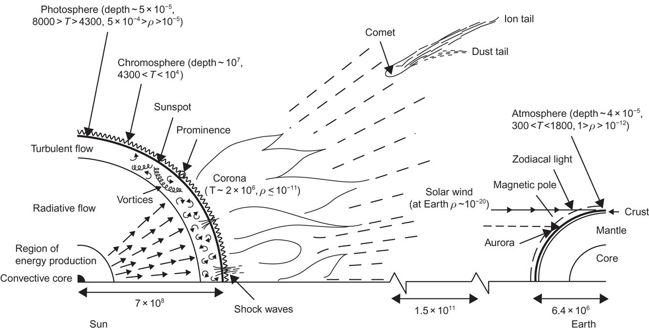
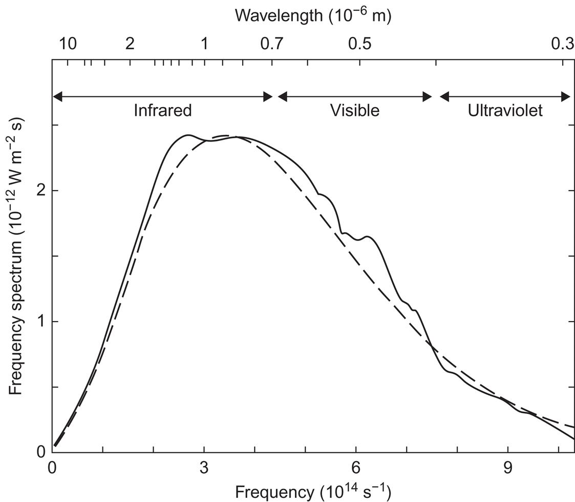
Practically all of the radiation from the Sun received at the Earth originates in the photosphere, a thin layer surrounding the convective mantle of high opacity. The depth to which a terrestrial observer can see the Sun lies in the photosphere. Owing to the longer path length in the absorptive region, the apparent brightness of the Sun decreases toward the edges. The photosphere consists of atoms of varying degree of ionization, plus free electrons. A large number of scattering processes take place, leading to a spectrum similar to the Planck radiation (2.3) for a blackbody in equilibrium with a temperature T≈6000 K. However, this is not quite so, partly because of sharp absorption lines corresponding to the transitions between different electron configurations in the atoms present (absorption lines of over 60 elements have been identified in the solar spectrum), and partly because of the temperature variation through the photosphere, from around 8000 K near the convective zone to a minimum of 4300 K at the transition to the chromosphere (see Fig. 2.7). Yet the overall picture, shown in Fig. 2.8, is in fair agreement with the Planck law for an assumed effective temperature Teff≈5762 K, disregarding in this figure the narrow absorption lines in the spectrum.
2.1.2.1 The structure of the solar surface
The turbulent motion of the convective layer underneath the Sun’s surface manifests itself in the solar disc as a granular structure interpreted as columns of hot, vertical updrafts and cooler, downward motions between the grain-like structures (supported by observations of Doppler shifts). Other irregularities of solar luminosity include bright flares of short duration, as well as sunspots, regions near the bottom of the photosphere with lower temperature, appearing and disappearing in a matter of days or weeks in an irregular manner, but statistically periodic (with an 11-year period). Sunspots first appear at latitudes at or slightly above 30°, reach maximum activity near 15° latitude, and end the cycle near 8° latitude. The “spot” is characterized by churning motion and a strong magnetic flux density (0.01–0.4 Wb m−2), suggesting its origin from vorticity waves traveling within the convective layer, and the observation of reversed magnetic polarity for each subsequent 11-year period suggests a true period of 22 years.
Above the photosphere is a less dense gas with temperature increasing outward from the minimum of about 4300 K. During eclipses, the glow of this chromosphere is visible as red light. This is because of the intense Hα line in the chromospheric system, consisting primarily of emission lines.
After the chromosphere comes the corona, still less dense (on the order of 10−11 kg m−3 even close to the Sun), but of very high temperature (2×10⁶ K, cf. Fig. 2.7). The mechanism of heat transfer to the chromosphere and to the corona is believed to be shock waves originating in the turbulent layer (Pasachoff, 1973). The composition of the corona (and chromosphere) is believed to be similar to that of the photosphere, but owing to the high temperature in the corona, the degree of ionization is much higher, and, for example, the emission line of Fe13+ is among the strongest observed from the corona (during eclipses). A continuous spectrum (K-corona) and Fraunhofer absorption lines (F-corona) are also associated with the corona, although the total intensity is only 10−6 of that of the photosphere, even close to the Sun (thus the corona cannot be seen from the Earth’s surface except during eclipses, owing to the atmospheric scattering of photospheric light). Because of its low density, no continuous radiation is produced in the corona itself, and the K-corona spectrum is due to scattered light from the photosphere, where the absorption lines have been washed out by random Doppler shifts (as a result of the high kinetic energy).
The corona extends into a dilute, expanding flow of protons (ionized hydrogen atoms) and electrons known as solar wind. The increasing radial speed at increasing distances is a consequence of the hydrodynamic equations for the systems (the gravitational forces are unable to balance the pressure gradient; Parker, 1964). Solar wind continues for as long as the momentum flow is large enough not to be deflected appreciably by the magnetic fields of interstellar material. Presumably, solar wind penetrates the entire solar system.
2.1.2.2 Radiation received at the Earth
At the top of the Earth’s atmosphere, solar wind has a density of about 10−20 kg m−3, corresponding to roughly 107 hydrogen atoms per m3. The ions are sucked into the Earth’s magnetic field at the poles, giving rise to such phenomena as the aurorae borealis and to magnetic storms. Variations in solar activity affect the solar wind, which in turn affects the flux of cosmic rays reaching the Earth (many solar wind hydrogen ions imply larger absorption of cosmic rays).
Cosmic ray particles in the energy range 103–1012 MeV cross interstellar space in all directions. They are mainly protons, but produce showers containing a wide range of elementary particles when they hit an atmosphere.
Figure 2.9 summarizes a number of radiation sources contributing to the conditions at the Earth. Clearly, radiation from the Sun dominates the spectral distribution as well as the integrated flux. The next contributions, some six orders of magnitude down in the visible region, even integrated over the hemisphere, are also of solar origin, such as moonlight, airglow, and zodiacal light (originating in the Sun’s corona, being particularly visible at the horizon just before sunrise and just after sunset). Further down, in the visible regions of the spectrum, are starlight, light from our own galaxy, and, finally, extragalactic light.
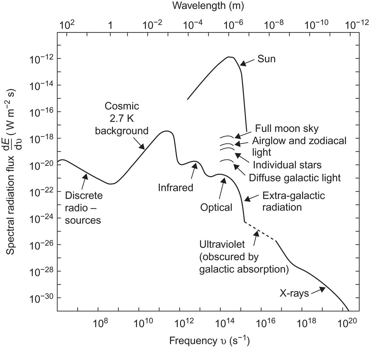
The peak in the spectral distribution of the extragalactic radiation is in the microwave region. This is the universal background radiation approximately following a Planck shape for 2.7 K, that is, the radiation predicted by, for example, the Big Bang theory of the expanding Universe.
The main part of solar radiation can be regarded as unpolarized at the top of the Earth’s atmosphere, but certain minor radiation sources, such as the light scattered by electrons in the solar corona, do have a substantial degree of polarization.
2.2 Disposition of radiation on the Earth
Solar radiation, which approximately corresponds to the radiation from a blackbody of temperature 6000 K, meets the Earth–atmosphere system and interacts with it, producing temperatures at the Earth’s surface that typically vary in the range of 220–320 K. The average (over time and geographical location) temperature of the Earth’s surface is presently 288 K.
As a first approach to understanding the processes involved, one may look at the radiation flux passing through unit horizontal areas placed either at the top of the atmosphere or at the Earth’s surface. The net flux is the sum (with proper signs) of the fluxes passing the area from above and from below. The flux direction toward the center of the Earth will be taken as positive, consistent with reckoning the fluxes at the Sun as positive, if they transport energy away from the solar center.
Since the spectral distributions of blackbody radiation (2.3) at 6000 and 300 K, respectively, do not substantially overlap, most of the radiation fluxes involved can be adequately discussed in terms of two broad categories, called short-wavelength (sw) and long-wavelength (lw) or thermal radiation.
2.2.1 Radiation at the top of the atmosphere
The flux of solar radiation incident on a surface placed at the top of the atmosphere depends on time (t) and geographical location (latitude φ and longitude λ) and on the orientation of the surface,
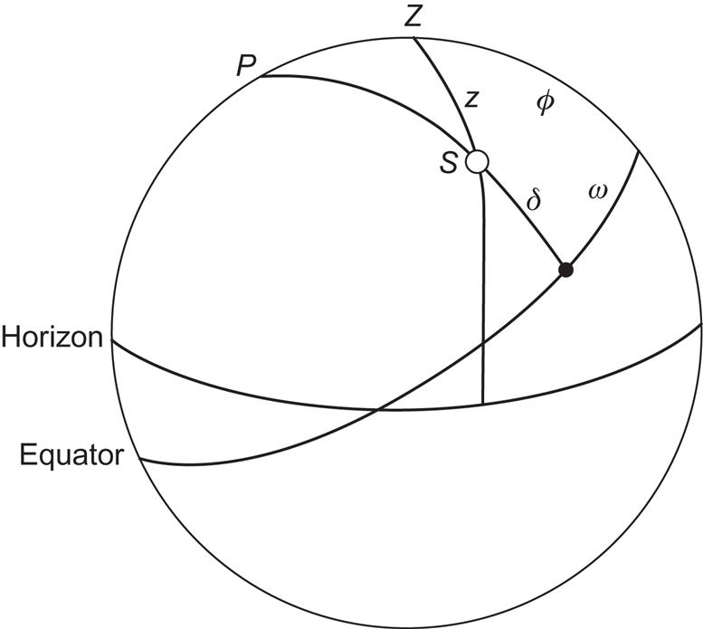
Here S(t) is the “solar constant” at the distance of the Earth (being a function of time, due to changes in the Sun–Earth distance and due to changes in solar luminosity) and θ is the angle between the incident solar flux and the normal to the surface considered. The subscript “0” on the short-wavelength flux Esw through the surface indicates that the surface is situated at the top of the atmosphere, and “+” indicates that only the positive flux (in the “inward” direction) is considered. For a horizontal surface, θ is the zenith angle z, obtained by
where δ is the declination of the Sun and ω is the hour angle of the Sun (see Fig. 2.10). The declination is given approximately by (Cooper, 1969)
(2.9)
where day is the actual day’s number in the year. The hour angle (taken as positive in the mornings) is related to the local time tzone (in hours) by
(2.10)
Here λzone is the longitude of the meridian defining the local time zone (longitudes are taken positive toward east; latitudes and declinations are positive toward north; all angles are in radians). The correction TEQ (equation of time) accounts for the variations in solar time caused by changes in the rotational and orbital motion of the Earth, e.g., due to speed variations in the elliptical orbit and to the finite angle (obliquity) between the axis of rotation and the normal to the plane or orbital motion. The main part of TEQ remains unaltered at the same time in subsequent years and may be expressed as a function of the day of the year (see Duffie and Beckman, 1974),
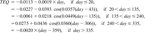
The resulting daily average flux on a horizontal surface,
which is independent of λ, is shown in Fig. 2.11. The maximum daily flux is about 40% of the flux on a surface fixed perpendicular to the direction of the Sun. It is obtained near the poles during midsummer, with light close to 24 hours of each day but a zenith angle of π/2−max(|δ|)≈67° (cf. Fig. 2.10, |δ| being the absolute value of δ). Daily fluxes close to 30% of the solar constant are found throughout the year at the Equator. Here the minimum zenith angle comes close to zero, but day and night are about equally long.
 + (W m−2), incident at the top of the Earth’s atmosphere, as a function of time of the year and latitude (independent of longitude). Latitude is (in this and the following figures) taken as positive toward north. Based on NCEP-NCAR (1998).
2.2.1.1 The disposition of incoming radiation
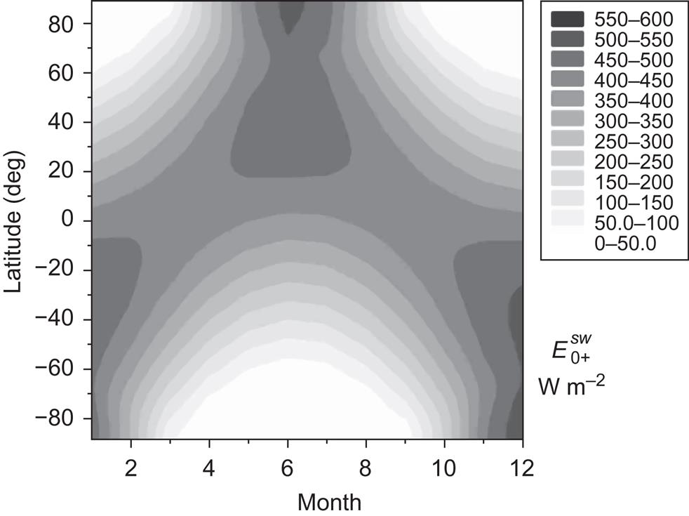
A fraction of the incoming solar radiation is reflected back into space. This fraction is called the albedo a0 of the Earth–atmosphere system. The year and latitude–longitude average of a0 is about 0.35. This is composed of about 0.2 from reflection on clouds, 0.1 from reflection on cloudless atmosphere (particles, gases), and 0.05 from reflection on the Earth’s surface. Figure 2.12 gives the a0 distribution for 2 months of 1997, derived from ongoing satellite measurements (cf. Wilson and Matthews, 1971; Raschke et al., 1973; NCEP-NCAR, 1998).
The radiation absorbed by the Earth–atmosphere system is
Since no gross change in the Earth’s temperature is taking place from year to year, it is expected that the Earth–atmosphere system is in radiation equilibrium, i.e., that it can be ascribed an effective temperature T0, such that the blackbody radiation at this temperature is equal to −A0,

Here S is the solar constant and σ=5.7×10⁻⁸ W m−2 K−4 is Stefan’s constant [cf. (2.4)]. The factor 1/4 is needed because the incoming radiation on the side of the Earth facing the Sun is the integral of S cosθ over the hemisphere, while the outgoing radiation is uniform over the entire sphere (by definition when it is used to define an average effective temperature). The net flux of radiation at the top of the atmosphere can be written
(2.11)
where ![]() on average equals −σT04 (recall that fluxes away from the Earth are taken as negative) and E0 on average (over the year and the geographical position) equals zero.
on average equals −σT04 (recall that fluxes away from the Earth are taken as negative) and E0 on average (over the year and the geographical position) equals zero.
The fact that T0 is 34 K lower than the actual average temperature at the Earth’s surface indicates that heat is accumulated near the Earth’s surface, due to re-radiation from clouds and atmosphere. This is called the greenhouse effect, and it is further illustrated below, in the discussion of the radiation fluxes at the ground.
The net radiation flux at the top of the atmosphere, E0, is a function of time as well as of geographical position. The longitudinal variations are small. Figure 2.13 gives the latitude distribution of ![]() ,
, ![]() , and
, and ![]() , where the reflected flux is
, where the reflected flux is
as well as ![]() :
:

 and outgoing long-wavelength
  radiation at the top of the atmosphere, the amount of radiation absorbed (A0) and reflected (R0) by the Earth–atmosphere system, and the net radiation flux E0 at the top of the atmosphere, in W m−2. Based on Sellers (1965); Budyko (1974).
Although ![]() is fairly independent of φ, the albedo
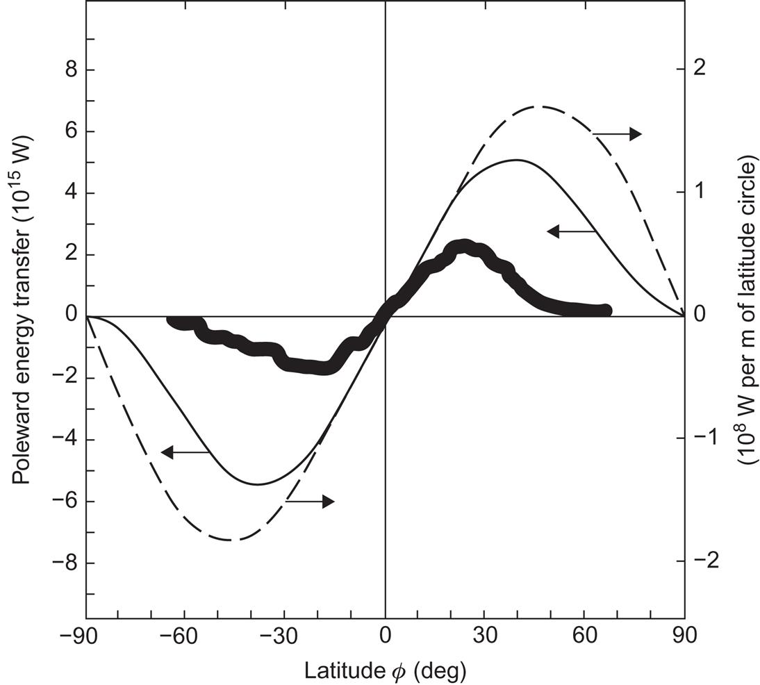
is fairly independent of φ, the albedo ![]() increases when going toward the poles. Most radiation is absorbed at low latitudes, and the net flux exhibits a surplus at latitudes below 40° and a deficit at higher absolute latitudes. Since no progressive increase in equatorial average temperatures, nor any similar decrease in polar temperatures, is taking place, there must be a transport of energy from low latitudes in the directions of both poles. The mechanisms for producing this flow are ocean currents and winds. The necessary amount of poleward energy transport, which is immediately given by the latitude variation of the net radiation flux (since radiation is the only mode of energy transfer at the top of the atmosphere), is given in Fig. 2.14, which also indicates the measured share of ocean transport. The total amount of energy transported is largest around |φ|=40°, but since the total circumference of the latitude circles diminishes as latitude increases, the maximum energy transport across a unit length of latitude circle is found at |φ|≈50°.
increases when going toward the poles. Most radiation is absorbed at low latitudes, and the net flux exhibits a surplus at latitudes below 40° and a deficit at higher absolute latitudes. Since no progressive increase in equatorial average temperatures, nor any similar decrease in polar temperatures, is taking place, there must be a transport of energy from low latitudes in the directions of both poles. The mechanisms for producing this flow are ocean currents and winds. The necessary amount of poleward energy transport, which is immediately given by the latitude variation of the net radiation flux (since radiation is the only mode of energy transfer at the top of the atmosphere), is given in Fig. 2.14, which also indicates the measured share of ocean transport. The total amount of energy transported is largest around |φ|=40°, but since the total circumference of the latitude circles diminishes as latitude increases, the maximum energy transport across a unit length of latitude circle is found at |φ|≈50°.
Figures 2.15 and 2.16 give the time and latitude dependence at longitude zero of the long-wavelength re-radiation, ![]() (since the flux is only in the negative direction), and net flux, E0, of the Earth–atmosphere system, as obtained from satellite measurements within the year 1997 (Kalnay et al., 1996; NCEP-NCAR, 1998). A0 may be obtained as the difference between
(since the flux is only in the negative direction), and net flux, E0, of the Earth–atmosphere system, as obtained from satellite measurements within the year 1997 (Kalnay et al., 1996; NCEP-NCAR, 1998). A0 may be obtained as the difference between ![]() : The latter equals the albedo (Fig. 2.12) times the former, given in Fig. 2.11.
: The latter equals the albedo (Fig. 2.12) times the former, given in Fig. 2.11.


2.2.2 Radiation at the Earth’s surface
The radiation received at the Earth’s surface consists of direct and scattered (plus reflected) short-wavelength radiation plus long-wavelength radiation from sky and clouds, originating as thermal emission or by reflection of thermal radiation from the ground.
2.2.2.1 Direct and scattered radiation
Direct radiation is defined as radiation that has not experienced scattering in the atmosphere, so that it is directionally fixed, coming from the disc of the Sun.
Scattered radiation is, then, the radiation having experienced scattering processes in the atmosphere. In practice, it is often convenient to treat radiation that has experienced only forward scattering processes together with unscattered radiation, and thus define direct and scattered radiation as radiation coming from, or not coming from, the direction of the Sun. The area of the disc around the Sun used to define direct radiation is often selected in a way depending on the application in mind (e.g., the solid angle of acceptance for an optical device constructed for direct radiation measurement). In any case, “direct radiation” defined in this way will contain scattered radiation with sufficiently small angles of deflection, due to the finite solid angle of the Sun’s disc.
The individual scattering and absorption processes are discussed further below, but in order to introduce the modifications in the spectral distribution due to passage through the atmosphere, Fig. 2.17 shows the amount of radiation surviving at sea level for a clear day with the Sun in zenith. A large number of absorption lines and absorption bands can be seen in the low-frequency part of the spectrum (corresponding to wavelengths above 0.7×10⁻⁶ m). They are due to H2O, CO2, O2, N2O, CH4, and other, minor constituents of the atmosphere. At higher frequencies, the continuous absorption bands dominate, in particular those of O3. Around 0.5×10⁻⁶ m, partial absorption by O3 produces a dip in the spectrum, and below a wavelength of 0.3×10⁻⁶ m (the ultraviolet part of the spectrum) or a frequency above 9.8×10¹⁴ s−1, the absorption by ozone is practically complete.
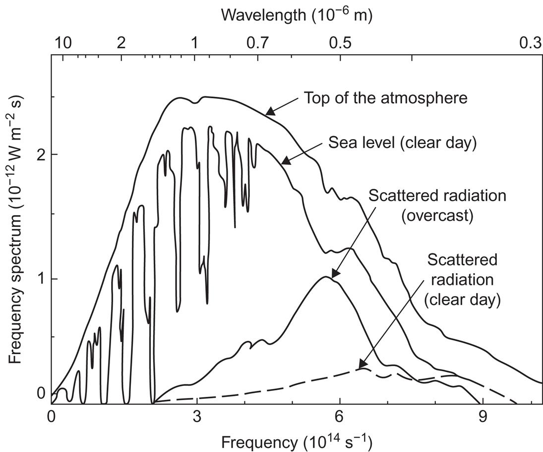
Figure 2.17 also shows the scattered part of the radiation on a clear day (dashed line). The scattered radiation is mainly composed of the most energetic (high-frequency) radiation, corresponding to the blue part of the visible spectrum. The sky on a clear day is therefore blue. The scattered light is also polarized. The radiation from clouds, i.e., from a completely overcast sky, is also shown in Fig. 2.17. It has a broad frequency distribution in the visible spectrum, so that the cloud light appears white.
2.2.2.2 Disposition of radiation at the Earth’s surface
On average, roughly half of the short-wavelength radiation that reaches the Earth’s surface has been scattered. Denoting the direct and scattered radiation at the Earth’s surface as D and d, respectively, and using the subscript s to distinguish the surface level (as the subscript “0” was used for the top of the atmosphere), the total incoming short-wavelength radiation at the Earth’s surface may be written
for a horizontal plane. The amount of radiation reflected at the surface is
where the surface albedo, as, consists of a part describing specular reflection (i.e., reflection preserving the angle between beam and normal to the rejecting surface) and a part describing diffuse reflection. Here diffuse reflection is taken to mean any reflection into angles different from the one characterizing beam reflection. An extreme case of diffuse reflection (sometimes denoted “completely diffuse” as distinguished from “partially diffuse”) is one in which the angular distribution of reflected radiation is independent from the incident angle.
The total net radiation flux at the Earth’s surface is
(2.12)
where the long-wavelength net radiation flux is
in terms of the inward and (negative) outward long-wavelength fluxes.
Figure 2.18 gives the latitude distribution of the incoming short-wavelength flux ![]() and its division into a direct, D, and a scattered part, d. The fluxes are year and longitude averages (adapted from Sellers, 1965). Similarly, Fig. 2.19 gives the total annual and longitude average of the net radiation flux at the Earth’s surface, and its components, as a function of latitude. The components are, from (2.12), the absorbed short-wavelength radiation,
and its division into a direct, D, and a scattered part, d. The fluxes are year and longitude averages (adapted from Sellers, 1965). Similarly, Fig. 2.19 gives the total annual and longitude average of the net radiation flux at the Earth’s surface, and its components, as a function of latitude. The components are, from (2.12), the absorbed short-wavelength radiation,
and the net long-wavelength thermal flux ![]() (Fig. 2.19 shows
(Fig. 2.19 shows ![]() ). The figures show that the direct and scattered radiation are of comparable magnitude for most latitudes and that the total net radiation flux at the Earth’s surface is positive except near the poles. The variations in the long-wavelength difference between incoming (from sky and clouds) and outgoing radiation indicate that the temperature difference between low and high latitudes is not nearly large enough to compensate for the strong variation in absorbed short-wavelength radiation.
). The figures show that the direct and scattered radiation are of comparable magnitude for most latitudes and that the total net radiation flux at the Earth’s surface is positive except near the poles. The variations in the long-wavelength difference between incoming (from sky and clouds) and outgoing radiation indicate that the temperature difference between low and high latitudes is not nearly large enough to compensate for the strong variation in absorbed short-wavelength radiation.

 , as functions of latitude. Adapted from Sellers (1965).
 and the net emission of long-wavelength radiation
  . Adapted from Sellers (1965).
The conclusion is the same as the one drawn from the investigation of the Earth–atmosphere net radiation flux. A poleward transport of heat is required, either through the Earth’s surface (e.g., ocean currents) or through the atmosphere (winds in combination with energy transfer processes between surface and atmosphere by means other than radiation).
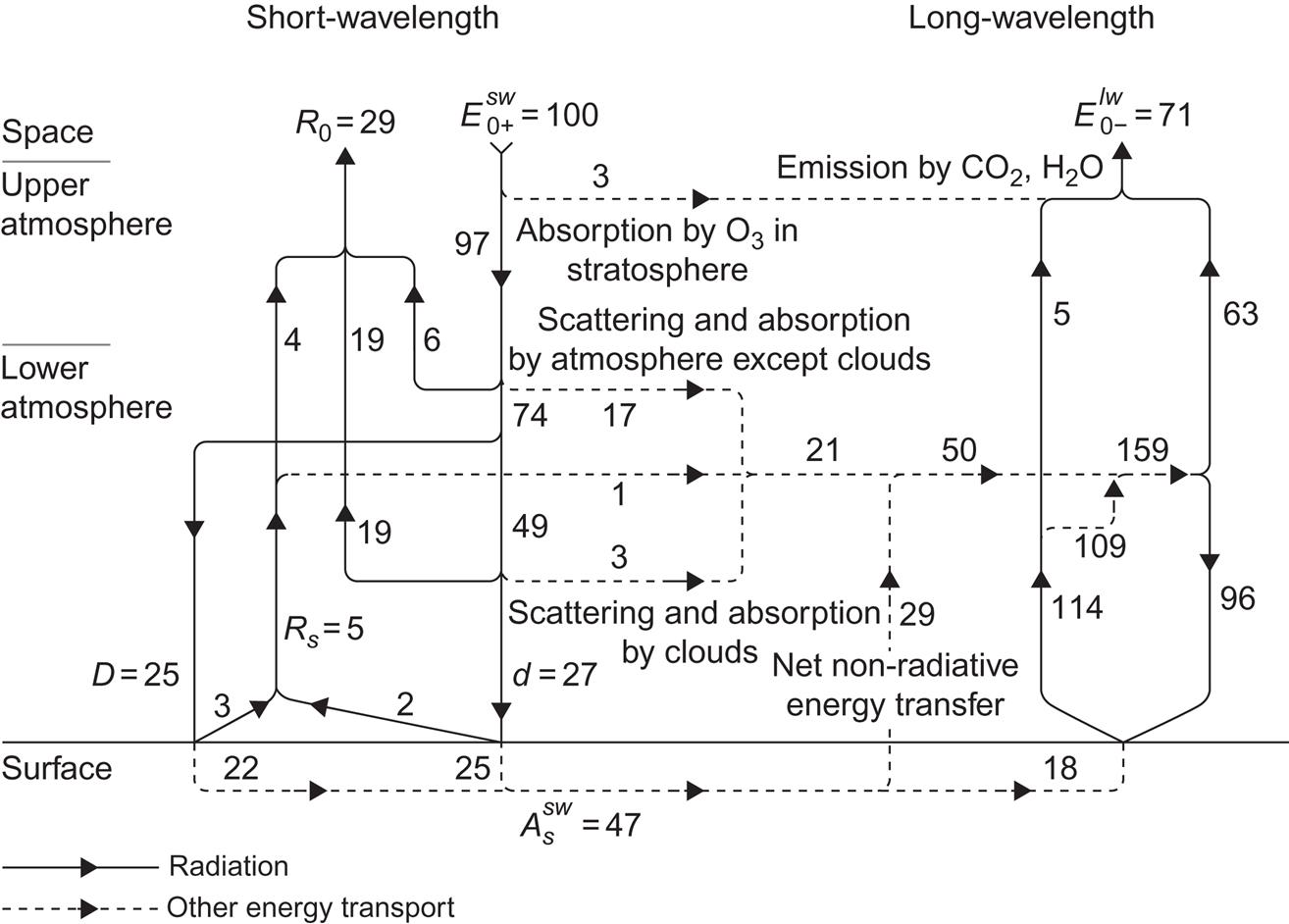
Figure 2.20 summarizes in a crude form the transfer processes believed to take place in the disposition of the incoming solar radiation. In the stratosphere, the absorption of short-wavelength radiation (predominantly by ozone) approximately balances the emission of long-wavelength radiation (from CO2, H2O, etc.). In the lower part of the atmosphere, the presence of clouds largely governs the reflection of short-wavelength radiation. On the other hand, particles and gaseous constituents of the cloudless atmosphere are most effective in absorbing solar radiation. All figures are averaged over time and geographical location.
 , put equal to 100 units) in the Earth–atmosphere system, averaged over time and geographical location. Symbols and details of the diagram are discussed in the text. The data are adapted from Sellers (1965); Budyko (1974); Schneider and Dennett (1975); Raschke et al. (1973).
Slightly over half the short-wavelength radiation that reaches the Earth’s surface has been scattered on the way. Of the 27% of the solar radiation at the top of the atmosphere that is indicated as scattered, about 16% has been scattered by clouds and 11% by the cloudless part of the sky.
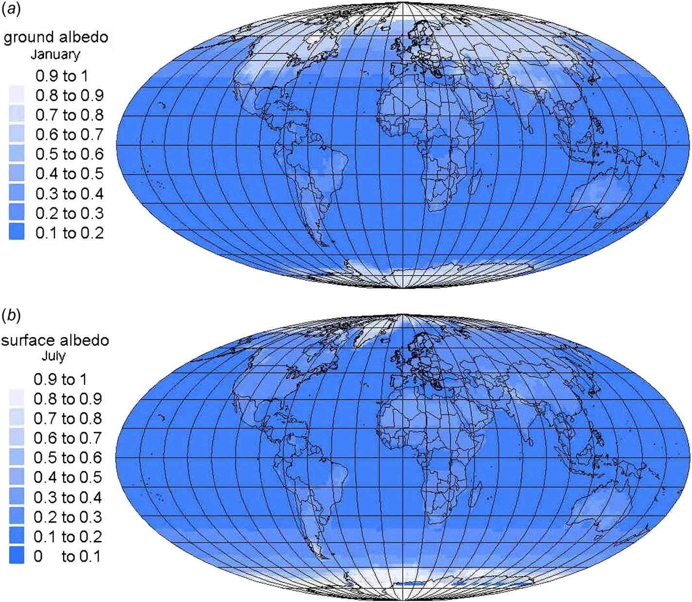
The albedo at the Earth’s surface is shown in Fig. 2.21 for 2 months of 1997, based on a re-analysis of measured data, using climate modeling to ensure consistency. The model has not been able to achieve full consistency of fluxes, probably because of too high albedo values over ocean surfaces (Kalnay et al., 1996). In Fig. 2.20 the average albedo is indicated as the smaller value as≈0.12. The albedo of a particular surface is usually a strongly varying function of the incident angle of the radiation. For seawater, the average albedo is about as=0.07, rising to about 0.3 in case of ice cover. For various land surfaces, as varies within the range 0.05–0.45, with typical mean values 0.15–0.20. In case of snow cover, as lies in the range 0.4–0.95, with the smaller values for snow that has had time to accumulate dirt on its surface.
As an illustration of the difficulties in estimating mean albedos, Fig. 2.22 shows the albedo of a water surface for direct sunlight, as a function of the zenith angle of the Sun. For a plane water surface and perpendicular incidence, the albedo implied by the air-to-water refraction index is 0.024. However, for ocean water, the surface cannot be regarded as a plane, and typical mean albedos (over the year) are of the order of 0.06, except at high latitudes, where the value may be greater. This estimate includes direct as well as scattered incident light, with the latter “seeing” a much more constant albedo of the water, of about 0.09 (Budyko, 1974).

The total amount of direct and scattered light, which in Fig. 2.20 is given as reflected from the ground, is a net value representing the net reflected part after both the initial reflection by the ground and the subsequent back-reflection (some 20%) from the clouds above, and so on.
2.2.2.3 Disposition of radiation in the atmosphere
On average, only a very small fraction of the long-wavelength radiation emitted by the Earth passes unhindered to the top of the atmosphere. Most is absorbed in the atmosphere or by clouds, from which the re-radiation back toward the surface is nearly as large as the amount received from the surface.
The net radiation flux of the atmosphere,
equals on average −29% of ![]() . The short-wavelength radiation absorbed is
. The short-wavelength radiation absorbed is ![]() , whereas the long-wavelength radiation absorbed and emitted in the lower atmosphere is
, whereas the long-wavelength radiation absorbed and emitted in the lower atmosphere is ![]() and
and ![]() , respectively. Thus, the net long-wavelength radiation is
, respectively. Thus, the net long-wavelength radiation is ![]() .
.
The net radiation flux of the atmosphere is on average equal to, but (due to the sign convention adopted) of opposite sign to, the net radiation flux at the Earth’s surface. This means that energy must be transferred from the surface to the atmosphere by means other than radiation, such as by conduction and convection of heat, by evaporation and precipitation of water and snow, etc. These processes produce energy flows in both directions, between surface and atmosphere, with a complex dynamic pattern laid out by river run-off, ocean currents, and air motion of the general circulation. The average deviation from zero of the net radiation flux at the surface level gives a measure of the net amount of energy displaced vertically in this manner, namely, 29% of ![]() or 98 W m−2. As indicated in Fig. 2.18, the horizontal energy transport across a 1-m wide line (times the height of the atmosphere) may be a million times larger. The physical processes involved in the transport of energy are discussed further in section 2.3.
or 98 W m−2. As indicated in Fig. 2.18, the horizontal energy transport across a 1-m wide line (times the height of the atmosphere) may be a million times larger. The physical processes involved in the transport of energy are discussed further in section 2.3.
2.2.2.4 Annual, seasonal, and diurnal variations in the radiation fluxes at the Earth’s surface
In discussing the various terms in the radiation fluxes, it has tacitly been assumed that averages over the year or over longitudes or latitudes have a well-defined meaning. However, as is well known, the climate is not completely periodic with a 1-year cycle, even if solar energy input is to a very large degree. The short-term fluctuations in climate seem to be very important, and the development over a time scale of a year depends to a large extent on the detailed initial conditions. Since, owing to the irregular short-term fluctuations, initial conditions at the beginning of subsequent years are not exactly the same, the development of the general circulation and of the climate as a whole does not repeat itself with a 1-year period. Although the gross seasonal characteristics are preserved as a result of the outside forcing of the system (the solar radiation), the year-average values of such quantities as mean temperature or mean cloudiness for a given region or for the Earth as a whole are not the same from one year to the next.
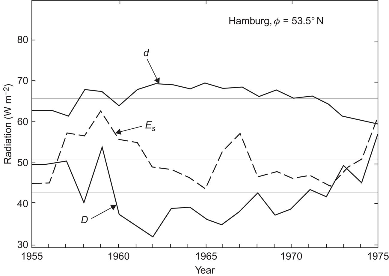
This implies that the components of the net radiation flux do not have the same annual average values from year to year. In particular, the disposition of incoming radiation as rejected, scattered, direct, and absorbed radiation is very sensitive to variations in cloud cover, and, therefore, exhibits substantial changes from year to year. Figure 2.23 shows the variations of yearly means of direct and scattered radiation measured at Hamburg (Kasten, 1977) over a 20-year period. Also shown is the variation of the net radiation flux at the ground. The largest deviation in direct radiation, from the 20-year average, is over 30%, whereas the largest deviation in scattered radiation is 10%. The maximum deviation of the net radiation flux exceeds 20%.
Figures 2.24 and 2.25 give, for different seasons in 1997, the total short-wavelength radiation (D+d) and the long-wavelength radiation fluxes ![]() at the Earth’s surface, as a function of latitude and longitude.
at the Earth’s surface, as a function of latitude and longitude.
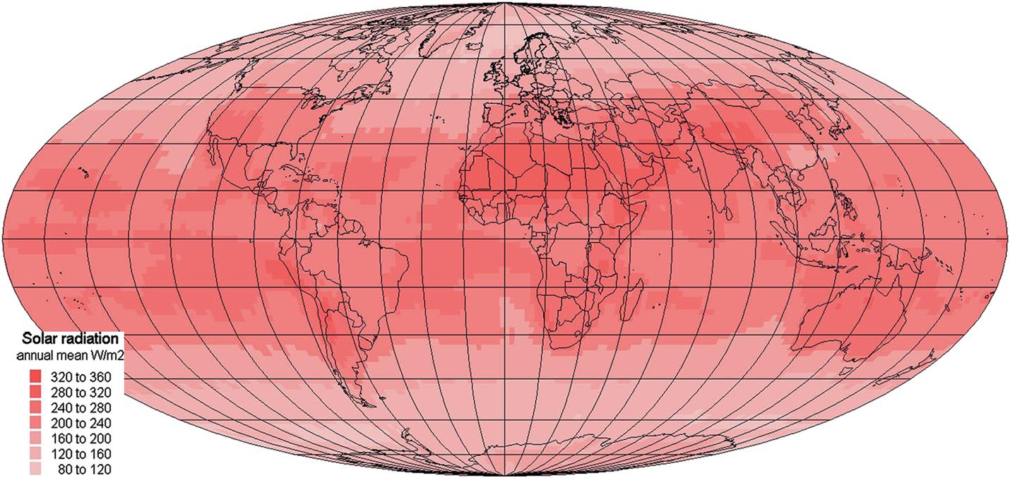
 on a horizontal surface at the Earth’s surface, as a function of geographical position (W m−2). (Based on NCEP-NCAR, 1998) Seasonal variations are shown in Chapter 3, Fig. 3.1.a–d.
 in January (a) and July (b), at the Earth’s surface, as a function of geographical position (W/m2). Based on NCEP-NCAR (1998).
Figure 2.26 gives the results of measurements at a specific location, Hamburg, averaged over 19 years of observation (Kasten, 1977). Ground-based observations at meteorological stations usually include the separation of short-wavelength radiation into direct and scattered parts, quantities that are difficult to deduce from satellite-based data. Owing to their importance for solar energy utilization, they are discussed further in Chapter 3. The ratio of scattered to direct radiation for Hamburg is slightly higher than the average for the latitude of 53.5° (see Fig. 2.18), and the total amount of incident short-wavelength radiation is smaller than average. This may be due to the climate modifications caused by a high degree of urbanization and industrialization (increased particle emission, increased cloud cover). On the other hand, the amount of short-wavelength radiation reflected at the surface, Rs, exceeds the average for the latitude.
 , the rejected part
  , and the flux of long-wavelength radiation received and emitted . Based on Kasten (1977).
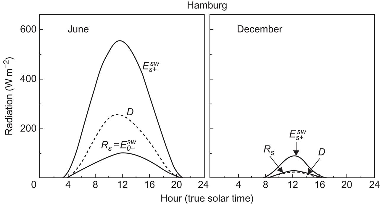
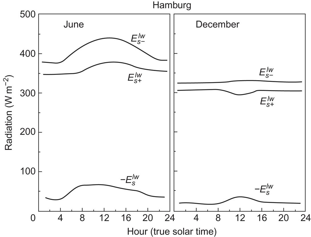
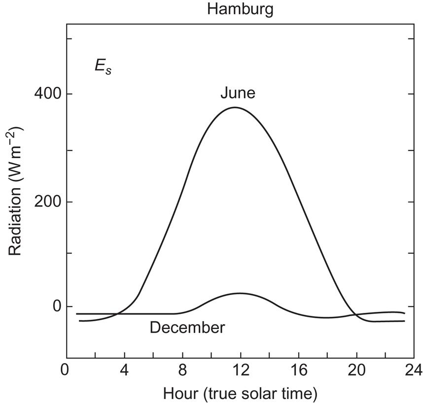
Figures 2.27–2.29 give the variations with the hour of the day of several of the radiation contributions considered above, again based on long-term measurements at Hamburg (Kasten, 1977). In Fig. 2.27, the incident radiation at ground level is shown for the months of June and December, together with the direct and reflected radiation. The mean albedo is about 0.18 at noon in summer and about 0.3 in winter. In December, the amount of reflected radiation exceeds the amount of direct radiation incident on the plane. The long-wavelength components, shown in Fig. 2.28, are mainly governed by the temperature of the ground. The net outward radiation rises sharply after sunrise in June and in a weakened form in December. In June, the separate outward and inward fluxes have a broad maximum around 14 h. The delay from noon is due to the finite heat capacity of the ground, implying a time lag between the maximum incident solar radiation and the maximum temperature of the soil. The downward flux changes somewhat more rapidly than the upward flux, because of the smaller heat capacity of the air. In December, the 24-h soil temperature is almost constant, and so is the outgoing long-wavelength radiation, but the re-radiation from the atmosphere exhibits a dip around noon. Kasten (1977) suggests that this dip is due to the dissolution of rising inversion layers, which during the time interval 16–08 h contributes significantly to the downward radiation. The hourly variation of the net total radiation flux is shown in Fig. 2.29 for the same 2 months. During daytime this quantity roughly follows the variation of incident radiation, but at night the net flux is negative, and more so during summer when the soil temperature is higher.
2.2.2.5 Penetration of solar radiation
In discussing the solar radiation absorbed at the Earth’s surface, it is important to specify how deep into the surface material, such as water, soil, or ice, the radiation is able to penetrate. Furthermore, the reflection of sunlight may take place at a depth below the physical surface.
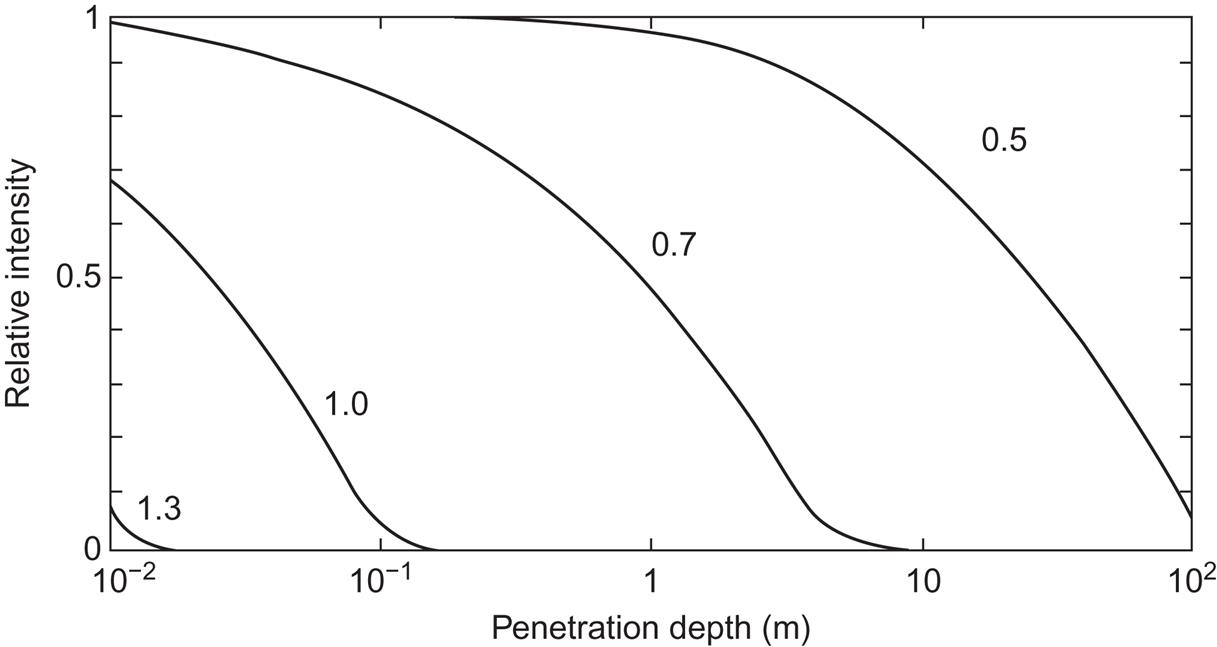
The penetration into soil, vegetation, sand, and roads or building surfaces is usually limited to at most 1 or 2 mm. For sand of large grain size, the penetration may reach 1–2 cm, in particular for the wavelengths above 0.5×10⁻⁶ m. For pure water, shorter wavelengths are transmitted more readily than longer ones. Figure 2.30 shows calculated intensity variations as a function of depth below the water’s surface and wavelength. The availability of solar radiation (although only about 5% of that incident along the normal to the water surface) at ocean depths of nearly 100 m is, of course, decisive for the photosynthetic production of biomass by phytoplankton or algae. For coastal and inland waters, the penetration of sunlight may be substantially reduced owing to dispersed sediments, as well as to eutrophication. A reduction in radiation intensity by a factor two or more for each meter penetrated is not uncommon for inland ponds (Geiger, 1961). The penetration of radiation into snow or glacier ice varies from a few tenths of a meter (for snow with high water content) to over a meter (ice).
2.3 Processes near the surface of the Earth
A very large number of physical and chemical processes take place near the Earth’s surface. No exhaustive description is attempted here, but emphasis is placed on those processes directly associated with, or important for, the possibility of utilizing the renewable energy flows in connection with human activities.
In particular, this leads to a closer look at some of the processes by which solar energy is distributed in the soil–atmosphere–ocean system, e.g., the formation of winds and currents. Understanding these processes is also required in order to estimate the possible climatic disturbance that may follow certain types of interference with the “natural” flow pattern.
Although the processes in the different compartments are certainly coupled, the following subsections first list a number of physical processes specific for the atmosphere, for the oceans, and, finally, for the continents and then indicates how they can be combined to account for the climate of the Earth.
2.3.1 The atmosphere
The major constituents of the present atmosphere are nitrogen, oxygen, and water. For dry air at sea level, nitrogen constitutes 78% by volume, oxygen 21%, and minor constituents 1%, the major part of which is argon (0.93%) and carbon dioxide (0.03%). The water content by volume ranges from close to zero at the poles to about 4% in tropical climates.
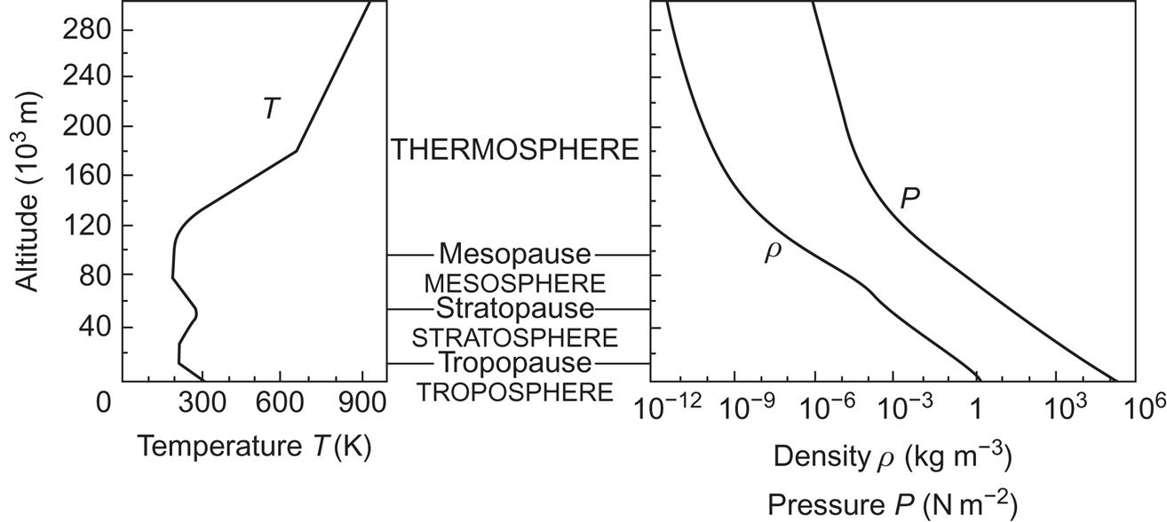
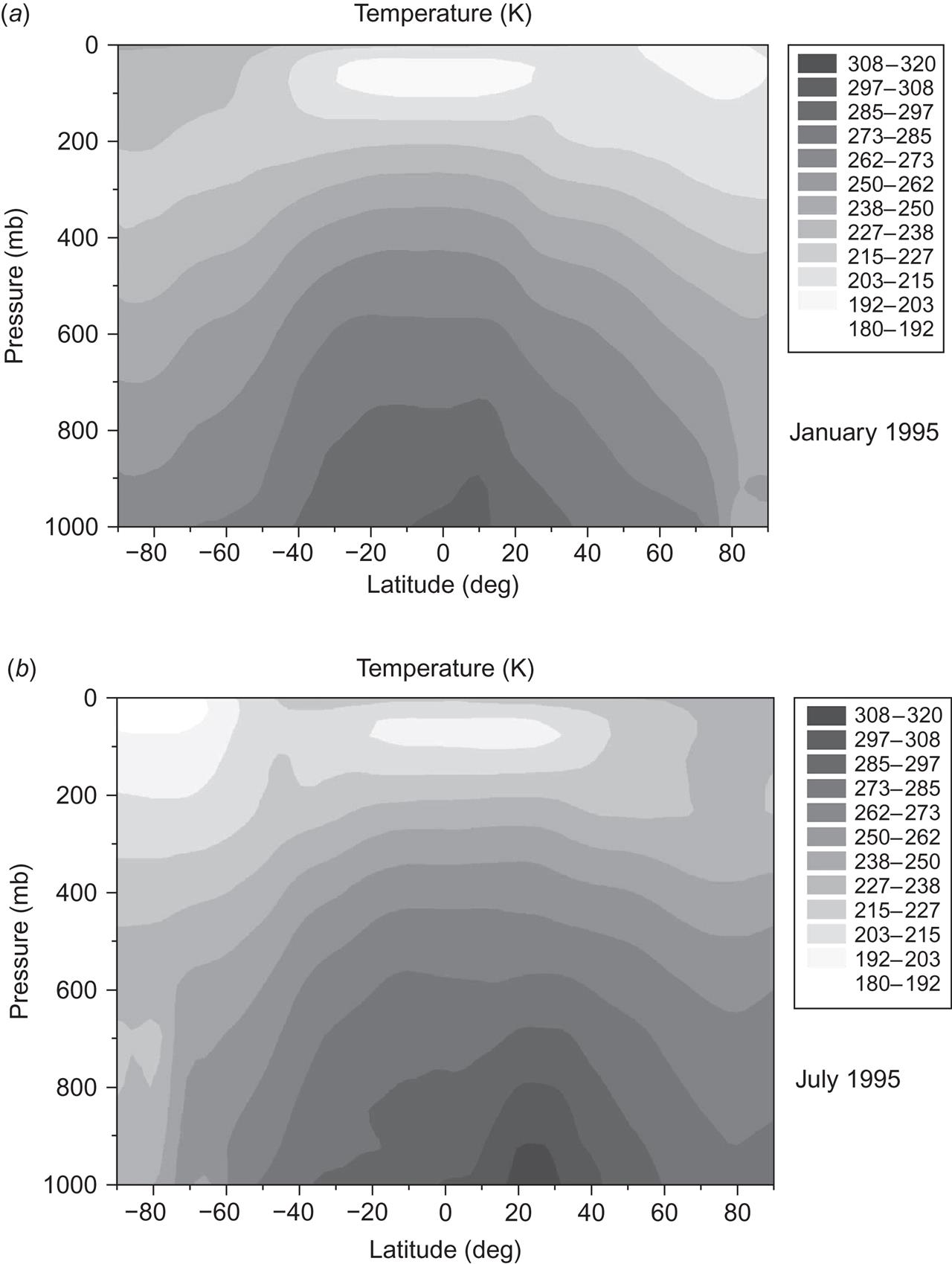
Typical variations of density, pressure, and temperature, as functions of altitude, are shown in Fig. 2.31. Common names for the different layers are indicated. They are generally defined by turning points in the temperature profile (“pauses”) or by the lower border of constant temperature regions if no sharp change in the sign of the temperature gradient takes place. Actual temperature profiles are not independent of latitude and season and do not exhibit sharp “turning points,” as indicated in Fig. 2.32.
Estimates of the variation with altitude of the average abundance of some gaseous constituents of the atmosphere are shown in Fig. 2.33. The increasing abundance of ozone (O3) between 15 and 25 km altitude is instrumental in keeping the level of ultraviolet radiation down, thereby allowing life to develop on the Earth’s surface (cf. Fig. 2.2). Above an altitude of about 80 km, many of the gases are ionized, and for this reason the part of the atmosphere above this level is sometimes referred to as the ionosphere. Charged particles occurring at the altitude of 60 000 km still largely follow the motion of the Earth, with their motion being mainly determined by the magnetic field of the Earth. This layer is referred to as the magnetosphere.

2.3.1.1 Particles in the atmosphere
In addition to gaseous constituents, water, and ice, the atmosphere contains particulate matter in varying quantity and composition. A number of mechanisms have been suggested for the production of particles varying in size from 10−9 to 10−4 m. One is the ejection of particles from the surface of the oceans, in the form of salt sprays. Others involve the transformation of gases into particles. This can occur as a result of photochemical reactions or as a result of adsorption to water droplets (clouds, haze), chemical reactions depending on the presence of water and finally evaporation of the water, leaving behind a suspended particle rather than a gas.
Dust particles from deserts or eroded soil also contribute to the particle concentration in the atmosphere, as does volcanic action. Man-made contributions are in the form of injected particles, from land being uncovered (deforestation, agricultural practice), industry, and fuel burning, and in the form of gaseous emissions (SO2, H2S, NH3, etc.), which may be subsequently transformed into particles by the above-mentioned processes or by catalytic transformations in the presence of heavy metal ions, for example.
Wilson and Matthews (1971) estimate that yearly emission into, or formation within, the atmosphere of particles with a radius smaller than 2×10⁻⁵ m is in the range (0.9–2.6)×1012 kg. Of this, (0.4–1.1)×1012 kg is due to erosion, forest fires, sea-salt sprays, and volcanic debris, while (0.3–1.1)×1012 kg is due to transformation of non-anthropogenic gaseous emissions into particles. Anthropogenic emissions are presently in the range (0.2–0.4)×1012 kg, most of which is transformed from gaseous emissions.
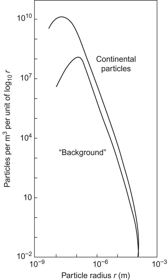
Figure 2.34 gives a very rough sketch of the particle density as a function of altitude. The distribution of large particles (radii in the range 10−7 to 2×10⁻⁵ m) is based on measurements at a given time and place (based on Craig, 1965), while the total particle counts are based on extrapolations of the size distribution to very small particles (see Fig. 2.35). It is clear that the total number of particles depends sensitively on the density of very small particles, which on the other hand do not contribute significantly to the total mass of particulate matter. The concentrations of rural and city particles in the right-hand part of Fig. 2.34 correspond to an extrapolation toward smaller radii of the size distributions in Fig. 2.35, such that the number of particles per m3 per metric decade of radius does not decrease rapidly toward zero.
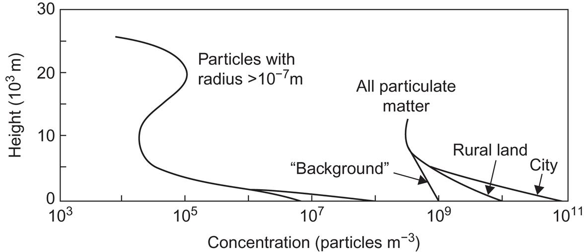
Returning to mass units, the total mass of particles in the atmosphere can be estimated from the emission and formation rates, if the mean residence time is known. The removal processes active in the troposphere include dry deposition by sedimentation (important only for particles with a radius above 10−6 m), diffusion, and impact on the Earth’s surface, vegetation, etc., and wet deposition by precipitation. The physical processes involved in wet deposition are condensation of water vapor on particles, in-cloud adsorption of particles to water droplets (called rainout), or scavenging by falling rain (or ice) from higher-lying clouds (called washout). Typically, residence times for particles in the troposphere are in the range 70–500 h (Junge, 1963), leading to the estimate of a total particle content in the atmosphere of the order of 1014 kg.
Particles may also be removed by chemical or photochemical processes, transforming them into gases.
Particle residence times in the stratosphere are much longer than in the troposphere. Sulfates (e.g., from volcanic debris) dominate, and the particles are spread close to homogeneously over each hemisphere, no matter where they are being injected into the stratosphere. Residence times are of the order of years, and removal seems to be by diffusion into the troposphere at latitudes around 55°. This picture is based on evidence from major volcanic eruptions and from detonation of nuclear weapons of megaton size. Both of these processes inject particulate matter into the stratosphere. The particles in the stratosphere can be detected from the ground, because they modify the transmission of solar radiation, particularly close to sunrise or sunset, where the path length through the atmosphere is at its maximum. Figure 2.36 shows atmospheric transmittance at sunrise, measured in Hawaii before and after the major volcanic eruption of Mt. Agung on Bali in 1963. The arrows indicate other eruptions that have taken place near the Equator during the following years and that may have delayed the return of the transmittance toward its value from before 1963.
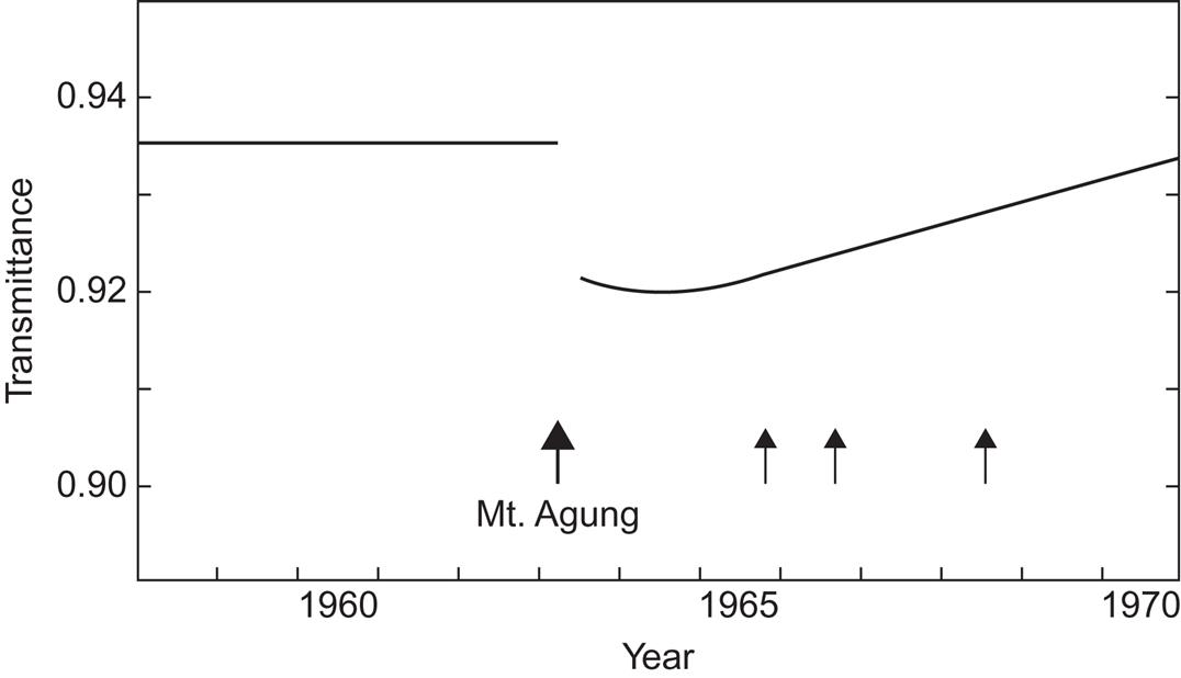
Figure 2.37 shows the ground deposition of radioactive debris (fallout), at latitude 56°N, after the enforcement of the test ban in 1963, which greatly reduced, but did not fully end, nuclear tests in the atmosphere. It can be concluded that the amount of radioactivity residing in the stratosphere is reduced by half each year without new injection. Observations of increased scattering (resulting in a shift toward longer wavelengths) following the very large volcanic eruption of Krakatoa in 1883 have been reported (sky reddening at sunrise and sunset). It is believed that the influence of such eruptions on the net radiation flux has had significant, although in the case of Krakatoa apparently transient, effects on the climate of the Earth.