where the square bracket denotes integer truncation.
The other wind-power average used in the regulation of the utility system is the average wind energy production in the previous 4 h, A4, which is used every hour in conjunction with the expected load for the following hour to make a trial estimate of the required number of intermediate-load units, ![]()
where the operation “integer” rounds to the closest integer number. This trial value is two units larger than the minimum value indicated by the predicted wind-power production, in order to make room for regulation of the intermediate-load units in both directions if the wind-power prediction should turn out to be inaccurate. The value of additional units is chosen as 2, because this is the number that, for the Danish power system, gives the smallest number of start-ups per year for the fuel-based units, in the absence of wind energy contributions. If the trial value, ![]() of intermediate-load units for the following hour exceeds the number already in use, a number of start-ups are so that the number of units actually operating 1 h later will be
of intermediate-load units for the following hour exceeds the number already in use, a number of start-ups are so that the number of units actually operating 1 h later will be ![]() If the number indicated by
If the number indicated by ![]() is smaller than the one already operating, it is not necessarily implemented; rather, the units already in operation are regulated downward. If it can be calculated that the regulation of all operating units down to the technical minimum level (assumed to be a third of the rated power) is insufficient, then one unit is stopped. It has been found advantageous on an annual basis not to stop more than one unit each consecutive hour, even if the difference between the minimum power production of the operating units and the expected demand will be lost. This is because of the uncertainty in the wind-power predictions, which in any case leads to losses of energy from the fuel-based units every time the wind-power production exceeds expectation by an amount that is too large to be counterbalanced by regulating the fuel-based units down to their technical minimum level (in this situation it is also permitted to regulate the base-load units). Not stopping too many of the intermediate-load units makes it easier to cope with an unexpected occurrence of a wind-power production below the predicted one during the following hour.
is smaller than the one already operating, it is not necessarily implemented; rather, the units already in operation are regulated downward. If it can be calculated that the regulation of all operating units down to the technical minimum level (assumed to be a third of the rated power) is insufficient, then one unit is stopped. It has been found advantageous on an annual basis not to stop more than one unit each consecutive hour, even if the difference between the minimum power production of the operating units and the expected demand will be lost. This is because of the uncertainty in the wind-power predictions, which in any case leads to losses of energy from the fuel-based units every time the wind-power production exceeds expectation by an amount that is too large to be counterbalanced by regulating the fuel-based units down to their technical minimum level (in this situation it is also permitted to regulate the base-load units). Not stopping too many of the intermediate-load units makes it easier to cope with an unexpected occurrence of a wind-power production below the predicted one during the following hour.
If the wind-power deficit is so large that, for a given hour, it cannot be covered even by regulating all fuel-based units in operation to maximum power level, then peak-load units must be called in. They can be fuel-based units with very short start-up times (some gas turbines and diesel units), hydropower units (with reservoirs), or “imports”, i.e., transfers from other utility systems through (eventually international) grid connections. [The role of international exchange in regulating a wind-power system has been investigated by Sørensen (1981), Meibom et al. (1997, 1999) and Sørensen (2015).] In a sufficiently large utility pool, there will always be units somewhere in the system that can be regulated upward at short notice. Another option is, of course, dedicated energy storage (including again hydro reservoirs).
All of these peak-load possibilities are in use within currently operated utility systems, and they are used to cover peaks in the expected load variation as well as unexpected load increases, and to make up for power production from suddenly disabled units (“outage”).
Summary of simulation results
Based on the 1-year simulation of the fuel-based system described above, with an installed capacity Iwind of wind energy converters added, a number of quantities are calculated. The installed wind energy capacity Iwind is defined as the ratio between annual wind energy production from the number of converters erected, ![]() given by (6.3), and the average load,
given by (6.3), and the average load,
(6.6)
The quantities recorded include the number of starts of the base- and intermediate-load units, the average and maximum number of such units in operation, and the average power delivered by each type of unit. For the peak-load facilities, a record is kept of the number of hours per year in which peak units are called and the average and the maximum power furnished by such units. Finally, the average power covered by wind is calculated. It may differ from the average production Iwind by the wind energy converters because wind-produced power is lost if it exceeds the load minus the minimum power delivered by the fuel-based units. If the annual average power lost is denoted Elost, the fraction of the load actually covered by wind energy, Cwind, may be written as
(6.7)
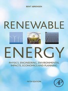
Figure 6.73 shows the average number of base- and intermediate-load unit start-up operations per unit and per year, as a function of Iwind. Also shown is the average number of base- and intermediate-load units in operation. The maximum number of base-load units operating is six, and the maximum number of base- plus intermediate-load units is 15.
Up to about Iwind=0.3, the wind energy converters are seen to replace mainly base-load units. The number of starts in the absence of wind energy converters is, on average, 35 per unit, rising to 98 for Iwind=0.3, and saturating at about 144.
In Fig. 6.74, the number of hours during which peak units are called is given, together with the maximum power drawn from such units in any hour of the year.

In the simulation, both of these quantities are zero in the absence of wind energy converters. This is an unrealistic feature of the model, since actual fuel-based utility systems do use peak-load facilities for the purposes described in the previous subsection. However, it is believed that the additional peak-load usage excluded in this way will be independent of whether the system comprises wind energy converters or not.
The number of peak unit calls associated with inappropriate wind predictions rises with installed wind capacity. For Iwind=0.25, it amounts to about 140 h per year or 1.6% of the hours, with a maximum peak power requirement that is about 40% of Eav. The asymptotic values for large Iwind are 1000 h per year (11.4%) and 155% of Eav.
The total amount of energy delivered by the peak units is not very large, as seen in Fig. 6.75. For Iwind up to about 0.4, it is completely negligible, and it never exceeds a few percent of the total annual load for any Iwind. This is considered important because the cost of fuels for peak-load units is typically much higher than for base- or intermediate-load units.
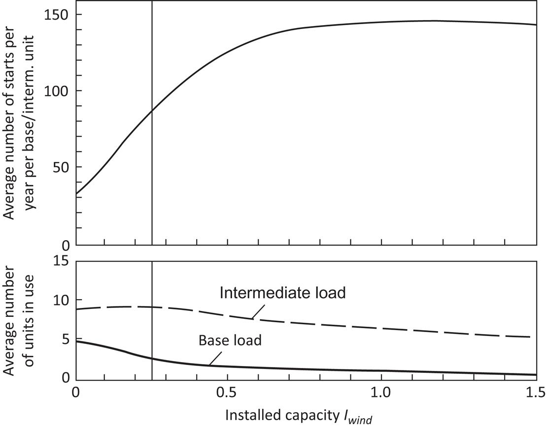
In Fig. 6.75, the fractional coverage by wind, base, intermediate, and peak units is shown as a function of Iwind, and the fraction of produced wind energy that is lost, Iwind−Cwind, is indicated as a shaded area. Up to an installed wind energy capacity of about Iwind=0.1, the lost fraction is negligible, and up to Iwind around 0.25, it constitutes only a few percent. For larger Iwind, the lost fraction increases rapidly, and the wind coverage, Cwind, actually approaches a maximum value of about 60%. Figure 6.75 also indicates how the wind energy converters first replace base-load units and affect the coverage by intermediate-load units only for larger Iwind.
Stochastic model
The regulation procedures described are quite rigorous, and one may ask how much the system performance will be altered if the prescriptions are changed. By modifying the prescription for choosing nbase, the relative usage of base- and intermediate-load units may be altered, and by modifying the prescription for choosing nint, the relative usage of intermediate- and peak-load units can be changed. The prescriptions chosen for nbase and nint give the smallest total number of starts of base plus intermediate units for zero wind contribution (Iwind=0).
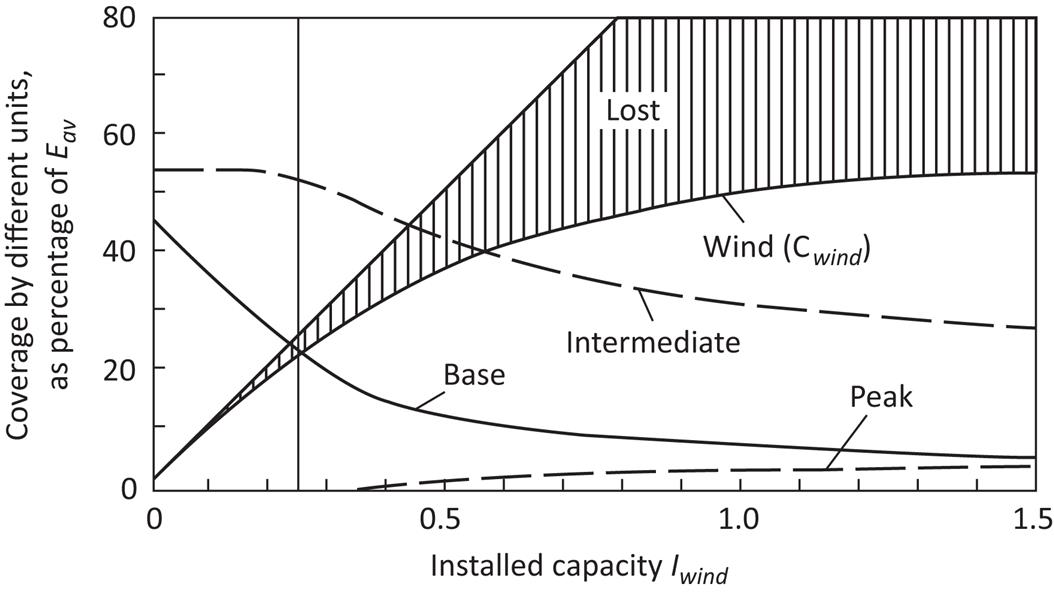
Also amenable to modification is the extrapolation procedure used to predict future wind energy production. Rather than using plain averages over the preceding 4 and 24 h (A4 and A24), one may try using a weighted average, which would emphasize the most recent hours more strongly. A number of such weighted averages were tried, one of which is illustrated in Fig. 6.76. Here A24 was replaced by (0.8A24+0.2A4) in the expression for nbase, and A4 was replaced by (0.8A4+0.2A1), A1 being the wind energy production for the preceding hour, in the expression for ![]() The resulting changes are very modest, for this as well as for other combinations tried, and no clear improvements over the simple averages are obtained in any of the cases.
The resulting changes are very modest, for this as well as for other combinations tried, and no clear improvements over the simple averages are obtained in any of the cases.
One may then ask if knowing the recent history of wind-power production is at all important for regulating the fuel-based back-up system. To demonstrate the non-random nature of the hour-to-hour variation in wind-power production, the predictive model based on previous average production was replaced by a stochastic model, which used the power production at a randomly selected time of the year, each time a prediction was required.
The basis for this procedure is a power duration curve [such as the ones in Fig. 6.69; however, for the present case, the Risø curve obtained by combining Fig. 3.40 and Fig. 6.70(a) was used]. A random number in the interval from zero to one (0%–100%) was generated, and the power-level prediction was taken as the power E from the power duration curve, which corresponds to the time fraction given by the random number. In this way, the stochastic model is consistent with the correct power duration curve for the location considered and with the correct annual average power. The procedure outlined was used to predict the power generation from the wind, to replace the averages A24 and A4 in the expressions for nbase and ![]()
The results of the stochastic model (c) are compared to those of the extrapolation type model (a) in Fig. 6.76. The most dramatic difference is in the number of start-ups required for the fuel-based units, indicating that a substantial advantage is achieved in regulating the fuel-based system by using a good predictive model for the wind-power contribution and that the extrapolation model serves this purpose much better than the model based on random predictions.
Some differences are also seen in the requirements for peak units, which are smaller for the extrapolation type model up to Iwind=0.3 and then larger. The latter behavior is probably connected with the lowering of the total wind coverage (bottom right in the figure) when using the stochastic model. This means that the number of fuel-based units started will more often be wrong, and when it is too high, more of the wind-produced power will be lost, the wind coverage will be lower, and the need for auxiliary peak power will be less frequent. The reason why these situations outnumber those of too few fuel-based units started, and hence an increased need for peak power, is associated with the form chosen for the nint regulating procedure. If this is the explanation for the lowering of the number of peak unit calls in the stochastic model for Iwind above 0.3 (upper right in Fig. 6.76), then the fact that the number of peak unit calls is lower for the extrapolation-type model than for the stochastic model in the region of Iwind below 0.3 implies that the extrapolation model yields incorrect predictions less often.
Economic evaluation of the requirements for additional start-ups, increased utilization of peak-load facilities, etc., of course, depends on the relative cost of such operations in the total cost calculation. For a particular choice of all such parameters, as well as fuel costs and the capital cost of the wind energy converters, a maximum installed wind capacity Iwind can be derived from the point of view of economic viability (cf. Chapter 7).
Wind-forecasting model
For the reasons explained in Chapter 2, general weather forecasts are inaccurate for periods longer than a few days, with the exact period depending on the strength of coupling between large-scale and chaotic atmospheric motion. For short periods, say under 12 h, the extrapolation methods described above in connection with time delays in starting up back-up power plants are expected to perform as well as meteorological forecasts based on general circulation models. Thus, the role of wind forecasting for power systems with wind-power is in the intermediate time range of 1–2 days. The interest in this interval has recently increased, due to establishment of power pools, where surpluses and deficits in power production are auctioned at a pool comprising several international power producers interconnected by transmission lines of suitable capacity. The Nordic Power Pool currently functions with a 36 h delay between bidding and power delivery. Therefore, the possibility of profitably selling surplus wind-power or buying power in case of insufficient wind depends on the ability to predict wind-power production 36 h into the future.
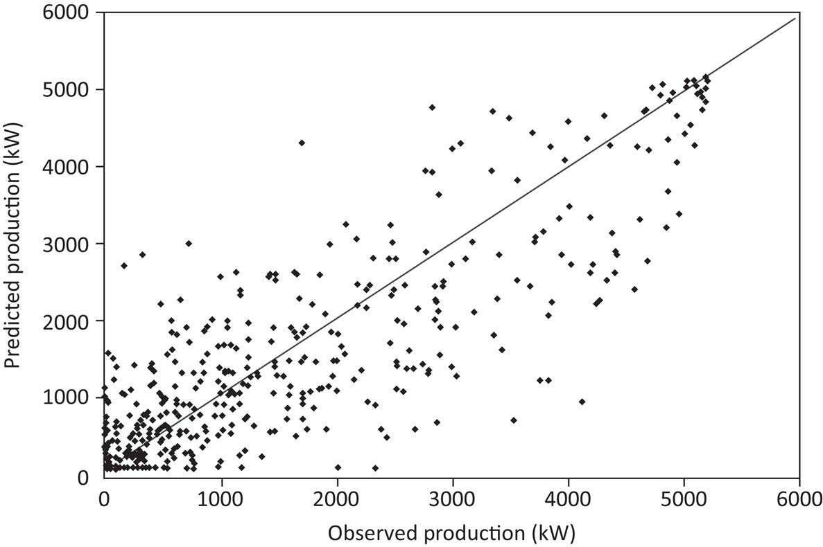
The quality of wind-power predictions, even for as little as 12 h, using the circulation models currently used in 1- to 5-day forecasts, is illustrated in Fig. 6.77. It clearly reflects the problem caused by non-linearity, as explained above. Yet, for the 36 h forecasts needed for bidding at the power pool, the average error of the forecasts of wind-power production (at Danish wind farms) is only 60% of that of extrapolation values (Meibom et al., 1997, 1999). The effect that this has on pool bidding is illustrated in Figs. 6.78 and 6.79 for a model in which the Danish power system is 100% based on wind-power, while the other Nordic countries primarily use hydropower, as today. Figure 6.69 shows the amount of wind-power buying and selling, after covering their own needs, for Eastern and Western Denmark. Figure 6.79 similarly gives the power duration curve for deviations of actual wind-power delivery from the bid submitted 36 h earlier. In terms of cost, using current trading prices at the Nordic Pool, incorrect bids will imply a monetary penalty amounting to 20% of the revenue from pool trade (this depends on a facility called the adjustment market, where additional bids for short-notice “regulation power” are used to avoid any mismatch between supply and demand). No other energy storage systems could presently provide back-up for wind-power at such a low cost.


6.5.2.3 Wind systems with short-term storage
All of the storage types mentioned in section 5.3 may be utilized as short-term stores in connection with wind energy systems. The purpose of short-term stores may be to smooth out the hourly fluctuations (the fluctuations on a minute or sub-minute scale being smoothed simply by having the system consist of several units of modest spacing). A back-up system must still be available if the extended periods of insufficient wind (typical duration one or a few weeks) are not to give rise to uncovered demands.
If the inclusion of short-term stores is to be effective in reducing the use of fuel-based peak-load facilities, it is important to choose storage types with short access times. It is also preferable for economic reasons to have high storage-cycle efficiency. This may be achieved for flywheel storage, pumped hydro storage, and superconducting storage (see Table 5.5).
A wind energy system including storage may be operated in different ways, such as:
i. Base-load operation. The system attempts to produce a constant power E0. If the production is above E0 and the storage is not full, the surplus is delivered to the storage. If the production is below E0 and the storage is not empty, the complementary power is drawn from the storage. If the production is above E0 and the storage is full, energy will be lost. If the production is below E0 and the storage is empty, the deficit has to be covered by auxiliary (e.g., fuel-based) generating systems.
ii. Load-following operation. The wind energy system attempts to follow the load (6.3), i.e., to produce power at a level E proportional to Eload,
If production by the wind energy converters is above the actual value of E and the storage is not full, the surplus is delivered to the storage. If the production is below E and the storage is not empty, the difference is drawn from the storage. Energy loss or need for auxiliary energy may arise as in (i).
iii. Peak-load operation. Outside the (somehow defined) time periods of peak load, all wind-produced energy is transferred to the storage facility. During the peak-load periods, a prescribed (e.g., constant) amount of power is drawn from the wind energy converters and their storage. Surplus production (if the storage is full) during off-peak hours may be transferred to the grid to be used to replace base or intermediate-load energy, if the regulation of the corresponding (fuel-based) units allows. A deficit during peak hours may, of course, occur. This system has two advantages. One is that the power to be used in a given peak-load period (say, 2 h) can be collected during a longer period (say, 10 h), because the probability of having adequate wind during part of this period is higher than the probability of having adequate wind during the peak hour, when the energy is to be used. The other advantage is that the wind energy in this mode of operation will be replacing fuel for peak-load units, i.e., usually the most expensive type of fuel. With respect to the first claimed advantage, the weight of the argument depends on the rating of the wind energy converters relative to their planned contribution to covering the peak load. If the wind energy converters chosen are very small, they would have to operate during most of the off-peak hours to provide the storage with sufficient energy. If they are very large, the advantage mentioned will probably arise, but, on the other hand, surplus energy that cannot be contained in the storage will be produced more often. It all depends, then, on the relative costs of the wind energy converters and the storage facilities. If the latter are low, a storage large enough to hold the produced energy at any time may be added, but if the storage costs are high relative to the costs of installing more converters, the particular advantage of an extended accumulation period may be decreased.
iv. Other modes of operation. Depending, among other things, on the installed wind energy capacity relative to the total load and on the load distribution, other schemes of operating a wind energy system, including short-term storage, may be preferable. For example, some fraction of the wind energy production may always be transferred to the storage, with the rest going directly to the grid. This may increase the probability that the storage will not be empty when needed. Alternatively, wind energy production above a certain fixed level may be transferred to the storage, but the system will still attempt to follow the actual load. There is also the possibility of having a certain fraction of the wind energy production in a load-following mode, but not all of it. Clearly, optimization problems of this type can be assessed by performing computer simulations.
6.5.3 Results of simulation studies
If short-term storage is added to a wind energy system in the base-load operation mode, the hourly sequence of power deliveries from the system may change as indicated in Fig. 6.72. On a yearly basis, the modifications may be summarized in the form of a modified power duration curve (compare Fig. 6.80 with the single-turbine curves in Fig. 6.69), where some of the “excess” power production occupying levels above average has been moved over to the region below the average level to fill up part of what would otherwise represent a power deficit.
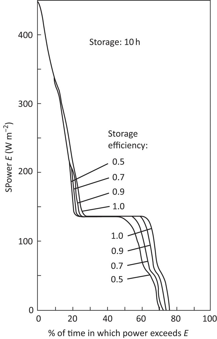
The results of Fig. 6.80 have been calculated on the basis of the 1961 Risø data (height 56 m), using the power coefficient curve (a) in Fig. 6.70, in an hour-by-hour simulation of system performance. The storage size is kept fixed at 10 h in Fig. 6.80 and is defined as the number of hours of average production (from the wind energy converters) to which the maximum energy content of the storage facility is equivalent. Thus, the storage capacity Ws may be written as
(6.8)
where Ws is in energy units and ts is the storage capacity in hours. E0 is the power level that the wind energy system in base-load operation mode aims at satisfying (for other modes of operation, E0 is the average power aimed at).
Storage-cycle efficiencies lower than unity are considered in Fig. 6.80, assuming for simplicity that the entire energy loss takes place when energy is drawn from storage. Thus, an energy amount W/ηs must be removed from the storage in order to deliver the energy amount W, where ηs is the storage-cycle efficiency.
The effect of the storage is to increase the fraction of time during which the power level E0 (or power levels 0<E≤E0) is available, causing the fractions of time during which the power level exceeds E0 to decrease. The availability of a given power level E is the time fraction tA(E), during which the power level exceeds E, and Fig. 6.81 shows the availability of the base-load power level, tA(E0), for the case of a loss-free storage (full line), as a function of storage capacity.
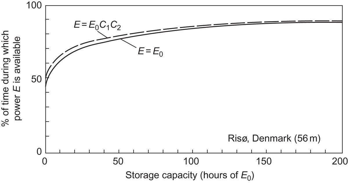
Thus, modest storage leads to a substantial improvement in availability, but improvements above availabilities of 75%–80% come much more slowly and require storage sizes that can no longer be characterized as short-term stores. However, the availabilities that can be achieved with short-term stores would be considered acceptable by many utility systems presently operating, owing to system structure and grid connections.
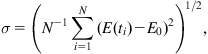
Another way to characterize the effect of adding a storage facility is to calculate the decrease in the average fluctuation σ of the system output E away from E0,
(6.9)
 (6.9)
(6.9)
where ti is the time associated with the ith time interval in the data sequence of N intervals. The annual fluctuation is given in Fig. 6.82 as a function of storage capacity ts, again for a loss-free storage.
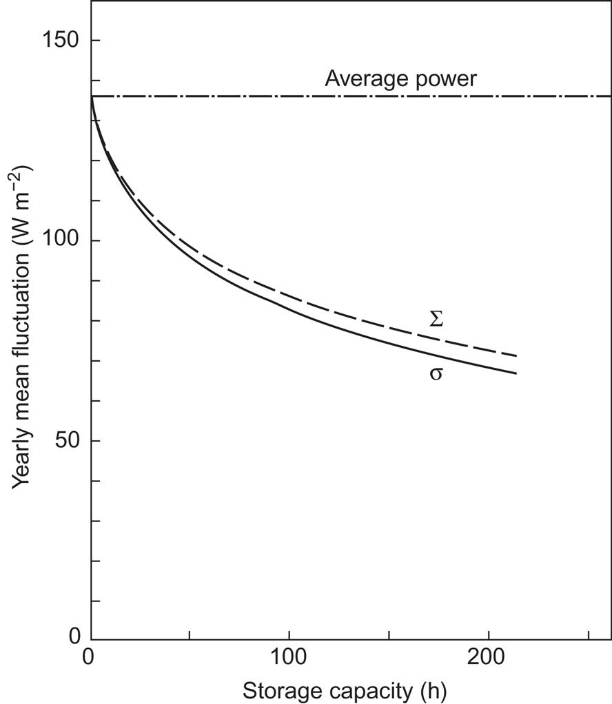
In the hourly simulation method, it is easy to keep track of the number of times that the operation of the storage switches from receiving to delivering power, or vice versa. This number is particularly relevant to those storage facilities whose lifetimes are approximately proportional to the number of charge/discharge cycles. Figure 6.83 gives the annual number of charge/discharge cycles, as a function of storage capacity, for the same assumptions as those made in Fig. 6.82.
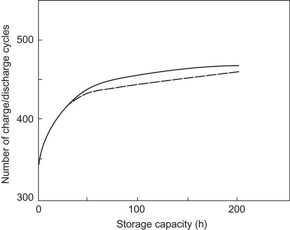
All these ways of illustrating the performance of a store indicate that the improvement per unit of storage capacity is high at first, but that each additional storage unit above ts≈70 h gives a very small return.
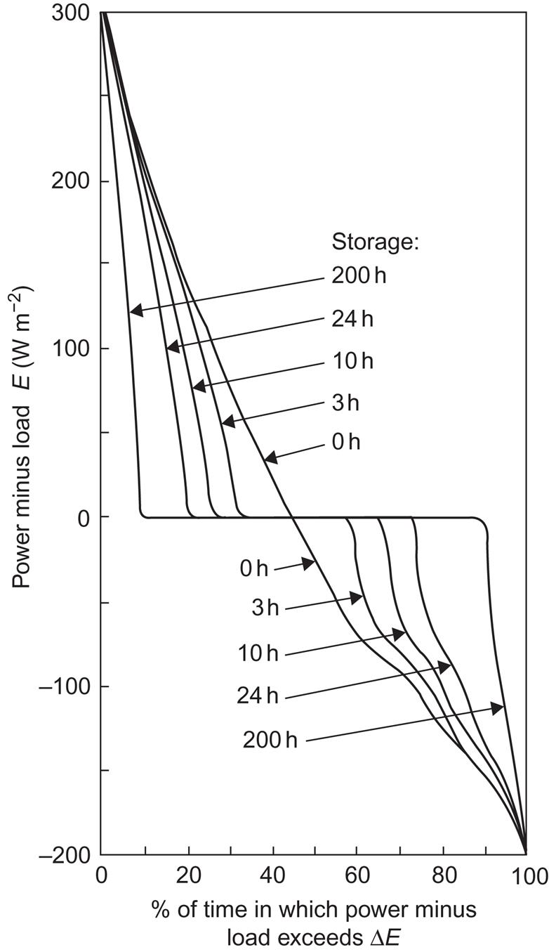
If the wind energy system including short-term storage is operated in a load-following mode, the storage size may still be characterized by ts derived from (6.8), but, in calculating fluctuations (called ∑ for convenience of distinction), E0 in (6.9) should be replaced by E0C1C2, and, in constructing a time duration curve, the relevant question is whether the power delivered by the system exceeds E0C1C2. Therefore, the power duration curve may be replaced by a curve plotting the percentage of time during which the difference E−E0C1C2 between the power produced at a given time, E, and the load-following power level aimed at, exceeds a given value ΔE. Such curves are given in Fig. 6.84 for an “average load” E0 equal to the annual average power production from the wind energy converters and assuming a loss-free store. The effect of augmenting storage capacity ts is to prolong the fraction of time during which the power difference defined above exceeds the value zero, i.e., the fraction of time during which the load aimed at can indeed be covered.
The results of load-following operation are also indicated in Figs. 6.81–6.83 (dashed lines), which show that the wind energy system actually performs better in the load-following mode than in the base-load mode, when a non-zero storage capacity is added.
Finally, Fig. 6.85 gives some results of operating a wind energy system with short-term storage in the peak-load mode, based on a simulation calculation performed by Coste (1976). The storage facility is imagined as an advanced battery type of cycle efficiency 70%. The system is aimed at delivering a constant peak-load power level, Epeak, but only during certain hours of the day and only on weekdays. The remaining time is used to accumulate energy in the storage whenever the wind energy converters are productive. If the storage units become filled, surplus generation may be delivered to the grid as off-peak power (at reduced credits). Figure 6.85 gives the storage capacity needed in this mode of operation in order to achieve an availability of 80%, as a function of the peak-load time fraction, i.e., the ratio between the accumulated time designed as peak-load periods and the total time period considered (1 year). The lack of continuity in the calculated points is due to dependence on the actual position of the peak-load hours during the day. It is determined by the load variation (cf. Fig. 6.14) and represents an increasing amount of “peak shaving” as the peak-load time fraction increases. This influences the length of accumulation times between peak-load periods (of which there are generally two, unevenly spaced over the day), which again is responsible for some of the discontinuity. The rest is due to the correlation between wind-power production and time of the day [cf. the spectrum shown in Fig. 3.37 or the average hourly variation, of which an example is given in Sørensen (1978a)], again in conjunction with the uneven distribution of the peak-load periods over the day.
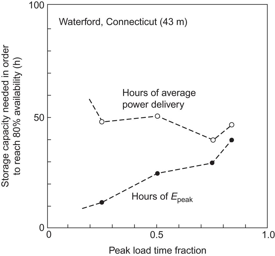
If the storage size is measured in terms of hours of peak-load power Epeak, the storage size required to reach an 80% availability increases with the peak-load time fraction, but, relative to the capacity of the wind energy converters, the trend is decreasing or constant. For small peak-load time fractions, the converter capacity is “small” compared to the storage size, because the accumulation time is much longer than the “delivery” time. In the opposite extreme, for a peak-load time fraction near unity, the system performs as in the base-load operation mode, and the storage size given as hours of Epeak coincides with those given in the previous figures in terms of E0.
6.5.3.1 Wind-power systems with long-term storage
Long-term storage is of interest in connection with wind energy systems aiming at covering a high fraction of the actual load. In this case, it is not possible to rely entirely on fuel-based back-up units to provide auxiliary power, and the wind energy system itself has to approach autonomy (to a degree determined by grid connections and the nature of the utility systems to which such connections exist).
The mode of operation used for wind energy systems that include long-term storage is therefore usually the load-following mode. A simple system of this sort uses pumped hydro storage (eventually sharing this storage system with a hydropower system, as mentioned earlier), in which case high storage-cycle efficiency can be obtained. The performance of such a system would be an extrapolation of the trends shown in Fig. 6.81.
In many cases, storage options using pumped hydro would not be available and other schemes would have to be considered (e.g., among those discussed in section 5.3). The best candidate for long-term storage and versatility in use is presently thought to be hydrogen storage (Gregory and Pangborn, 1976; Lotker, 1974; Bockris, 1975; Sørensen et al., 2004). The cycle efficiency is fairly low (cf. Table 5.5) for electricity regeneration by means of fuel cells (and still lower for combustion), but the fuel-cell units could be fairly small and could be placed in a decentralized fashion, so that the “waste heat” could be utilized conveniently (Sørensen, 1978a; Sørensen et al., 2004). The production of hydrogen would also provide a fuel that could become important in the transportation sector. The use of hydrogen for short-term storage has also been considered (Fernandes, 1974), but, provided that other short-term stores of higher cycle efficiency are available, a more viable system could be constructed by using storage types with high cycle efficiency for short-term storage and hydrogen for long-term storage only.
An example of the performance of a wind energy system of this kind is given in Fig. 6.86, using the simulation model described previously. A 10-hour storage (of average production E0, which has to exceed average load Eav owing to the storage losses) with 90% cycle efficiency is supplemented by long-term storage of assumed efficiency 50% (e.g., electrolysis-hydrogen-fuel cells), and the capacity of the long-term storage is varied until the minimum value that will enable the system to cover the total load at any time of the year is found. This solution, characterized by a power-minus-load duration curve that is positive 100% of the time, is seen to require a long-term storage of capacity tA(Eav)=1250 h. If the availability requirement is reduced to 97% of the time, the long-term storage size may be reduced to 730 h (1 month). Hydrogen storage in underground caverns or aquifers, which satisfies these requirements, is available in many locations (Sørensen et al., 2001, 2004; Sørensen, 2004).

6.6 Regional systems
In this section, scenarios for use of renewable energy are assessed on a regional basis. This means that the appraisal of energy demands and renewable energy supply options can be done on a regional basis, often with cultural similarities that make it easier to agree on the needs leading to energy demands. Furthermore, the possibility of exchanging energy between countries in the same region will alter the options for optimizing the system, as collaborative management of the system can reduce the need for each country in the region to install enough renewable energy to satisfy the highest demand. Generally, it will be cheaper to rely on the largest renewable energy sources in each country and to trade energy, either because a surplus capacity is fortuitously located in a country different from the one needing the energy or because the load peaks occur at different times, so that collaboration smoothes the necessary production in time.
Several examples are given: the Northern European region, which is special due to its high availability of (existing) hydro power, the Mediterranean region, the North American region, Japan-Korea, and China. For all these regions, a detailed assessment of available renewable energy supply options is made, with more fine-meshed methods than the ones used for the global models of section 6.7. For several of these regions, complete energy system scenarios are constructed, showing in detail the advantages of cooperating, with shared use of energy stores and exchange of power or fuels (biofuels or renewably produced hydrogen), whenever time-related performance can benefit from imports or exports. The importance of the trade options is illustrated by first designing an energy system for each country as if it were an island that has to solve all its energy-system problems by itself, and then see how trade can help. Today, exchange of power and fuels takes place regularly between countries, but in most cases it has to increase in magnitude to accommodate large inputs of renewable energy.
6.6.1 Regional scenario construction
Section 6.2 presented considerations for the construction of demand scenarios for use in scenarios for the future. This general category is termed precursor scenarios. To simplify the variety of scenario combinations, here it is assumed that the highest-efficiency intermediary-conversion scenario goes together with the highest-efficiency end-use scenario, and similarly that the lowest-efficiency choice applies both to intermediate and end-use conversion. Below is an outline of three such scenarios, corresponding to the range of behaviors anticipated in the precursor scenarios. The single load-scenario described in section 6.2.3 is used in the global scenarios discussed in Chapter 6.7. The regional scenarios discussed below in sections 6.6.2 to 6.6.4 choose the middle of the three end-use scenario alternatives made explicit below. It is interesting that, in some cases, new developments have made the middle-efficiency scenario closer to what 10 years ago would have been considered the highest-efficiency assumption.
6.6.1.1 The efficiency scenarios
Biologically acceptable surroundings
The fixed relationship between indoor temperature T and space heating or cooling requirement P (for power) assumed in section 6.2.3 for 60 m2 floor space per person (in work, home, and leisure heated or cooled spaces) was
This assumption corresponds to use of the best technology available in 1980. For the 2050–2060 scenarios, this is taken as the lowest, unregulated-efficiency scenario, realized by leaving the development to builders. Using instead the best technology available in Denmark by 2005, as a result of repeated but modest tightening of building codes, gives c=24 W/cap/°C. This lightly regulated development constitutes the middle-efficiency scenario, actually used in the examples of sections 6.6.2 to 6.6.5. The highest-efficiency scenario assumes a further technology improvement to take place and to be employed between now and the scenario year, yielding c=18 W/cap/°C.
Using the middle scenario requires delivery of space heating and cooling on an area base (for GIS calculations) at the rates of
as it is assumed that the dependence of the comfort temperature zone on outdoor temperature exhibits a ±4°C interval due to the flexible influence of indoor activities, as affected by body heat and clothing. The factor d is the population density, people per unit area (cap m−2), and P is thus expressed in W m−2.
Food, health, and security
In accord with section 6.2.3, an average end-user energy requirement of 120 W cap−1 for food, 18 W cap−1 for food storage, and small contributions for water supply, institutions, and security (police, military), are assumed to be included here or in the building and production energy figures. Only hot water for hygiene and clothes washing is different in the scenarios, amounting to an average of 100 W cap−1 in the high-efficiency scenario, 142 W cap−1 in the intermediate scenario used below (which is the same as used in the 1998 study; Sørensen et al., 2001), and 200 W cap−1 in the unregulated-efficiency scenario.
Human relations
Energy use for human relations and leisure activities at the end-user translated in the 1998 study to an average 100 W cap−1 and is chiefly electricity for lighting, telecommunications, electronic entertainment, and computing. Not anticipated at the time was the magnitude of demand increase: for instance, CRT computer and television screens were phased out and were replaced by flat screens of similar size that use less than 10% of the energy CRTs used. In reality, much of the energy gain was diminished by a perceived demand for larger screens (25-inch TV screens were replaced by 50-inch flat screens, greatly affecting the reduction in energy use) and more screens (most dwellings already approach one screen per room). One positive development is reduced equipment energy use when idling (in stand-by mode): sensors can switch off equipment (to stand-by) whenever there are no people in a particular room. That would return the energy use to one screen per capita. For computers (which have already replaced music and video players) this might also be the case, except for those that perform special services while unattended (burglary surveillance, satellite recording, and possibly plain computing, at least in the case of scientists). Furthermore, one screen may serve several inputs (switching between say a couple of computers and video inputs).
Consequently, the three demand scenarios used here have electricity use for relations set at 100, 200, and 300 W cap−1, typically derived from people’s three times higher rates of energy use during the 8 hours a day when they are not at work, commuting, or sleeping. Again, the middle-efficiency scenario is used in the regional scenarios. Currently, in affluent countries, such average end-use is a little above 100 W cap−1.
Heat energy for leisure-activities venues is assumed to be incorporated into the building’s heat use, while indirect uses for equipment, freight, and services are incorporated into the human activities energy use.
Transportation for human relations includes visits to family and friends, theaters, and concert venues, as well as vacations. When shopping is included, annual use today averages a total of about 10 000 km y−1 cap−1 (Sørensen, 2008b), with both short and long trips included. There is a large spread, and the scenarios assume 8000, 16 000, and 24 000 km y−1 cap−1 for non-work-related travel. Distances traveled are translated into energy units by using 0.04 W/(km y−1) for personal transport and 0.1 W/(ton-km y−1) for freight transport. These values correspond to state-of-the-art vehicles used at present.
Human activities
Non-leisure activities are what humans do in exchange for food and leisure provision. They include the devices involved (vehicles, washing machines, and computers, and so on), which have to be manufactured. Furthermore, manufacturing requires a range of raw materials that have to be obtained (e.g., by mining). Energy is one such requirement. Section 6.2.3 lists a range of such indirect demands. Because there are many ways to arrive at a particular product, the manufacturing techniques and inputs change with time. Innovation can follow different directions and is at times very rapid and thus difficult to predict in a scenario context. Technological change also has a non-technical component: for example, when we change our behavior to avoid diminishing animal diversity, or to avoid pesticides in our food intake and skin care products by choosing ecological (organic) produce or products. The negative effects of certain energy systems can also induce altered preferences, such as selecting “green electricity” rather than nuclear or coal electricity (a choice given by several power utilities). All these considerations should be reflected in the range of human activity scenarios offered.
Indirect activities for food and leisure equipment production, for distribution and sale of products, as well as for building and infrastructure construction and consequently materials provision, are estimated in section 6.2.3 to comprise some 60 W cap−1 of mainly high-quality energy (electric or mechanical energy), plus 3000 ton-km y−1 cap−1 of goods transportation plus 10 000 km y−1 cap−1 of work-related passenger transportation (e.g., in the service sector). These are all to be included in the activities energy use. The transportation figures translate into 400 W cap−1 average power use for person-transport and 300 W cap−1 for freight transportation. These numbers are taken as describing the highest-efficiency scenario.
The middle-efficiency scenario assumes 120 W cap−1 for agriculture and industry (for countries concentrating on information technologies, cf. Fig. 6.1), 600 W cap−1 for work-related transport (commuting included), and 400 W cap−1 for freight transportation, and the unregulated-efficiency scenario, 180 W cap−1, 1000 W cap−1, and 500 W cap−1, respectively. The high values for business-related personal transportation are caused by insistence on personal-contact meetings instead of videoconferences. The high values for transportation in the unregulated scenario imply a similar high use of time, which may be undesirable to business and industry unless travel time can be used productively (e.g., in trains and planes). People already complain about time wasted in personal car travel (such as commuting to and from work). One solution could be to make the employer responsible for transporting employees to and from work (presumably leading to selection of energy-efficient solutions) and including commuting time as work hours (because otherwise the employer could impose on employees’ leisure time by choosing slow but cheap transportation solutions).
6.6.2 Northern Europe
A very detailed study, mapping energy supply and demand on a geographical grid of 0.5 km×0.5 km, has been made for Denmark for an energy-efficient 2050 scenario. It is described in Sørensen (2005). Here an update of that study is looked at, expanding the region considered to the Nordic countries (except Iceland) and Germany. The new study uses the methodology described in section 6.6.1, choosing the middle-efficiency scenario as in section 6.6.2. The region is interesting because of the large amount of hydro with seasonal reservoirs present in Norway and Sweden, and because of the much higher population and energy-use density in Germany and Denmark, compared to the other three countries. Denmark has generous supplies of wind and agricultural energy, Sweden and Finland have similar supplies of forestry energy, and Norway and Finland have particularly good supplies of wind energy. Germany has reasonable agricultural assets, but its wind resources are only on the northern shores. Some solar energy can be derived, particularly in the south, but there remains a large deficit in electricity provision. However, as the study concludes, the surplus of energy in the Nordic countries is more than twice as large as the deficit in Germany, implying that German supply and demand can be balanced either by importing electricity from wind or hydro, or by importing less electricity and more biofuels, eventually with some final conversions (e.g., to hydrogen) in Germany.
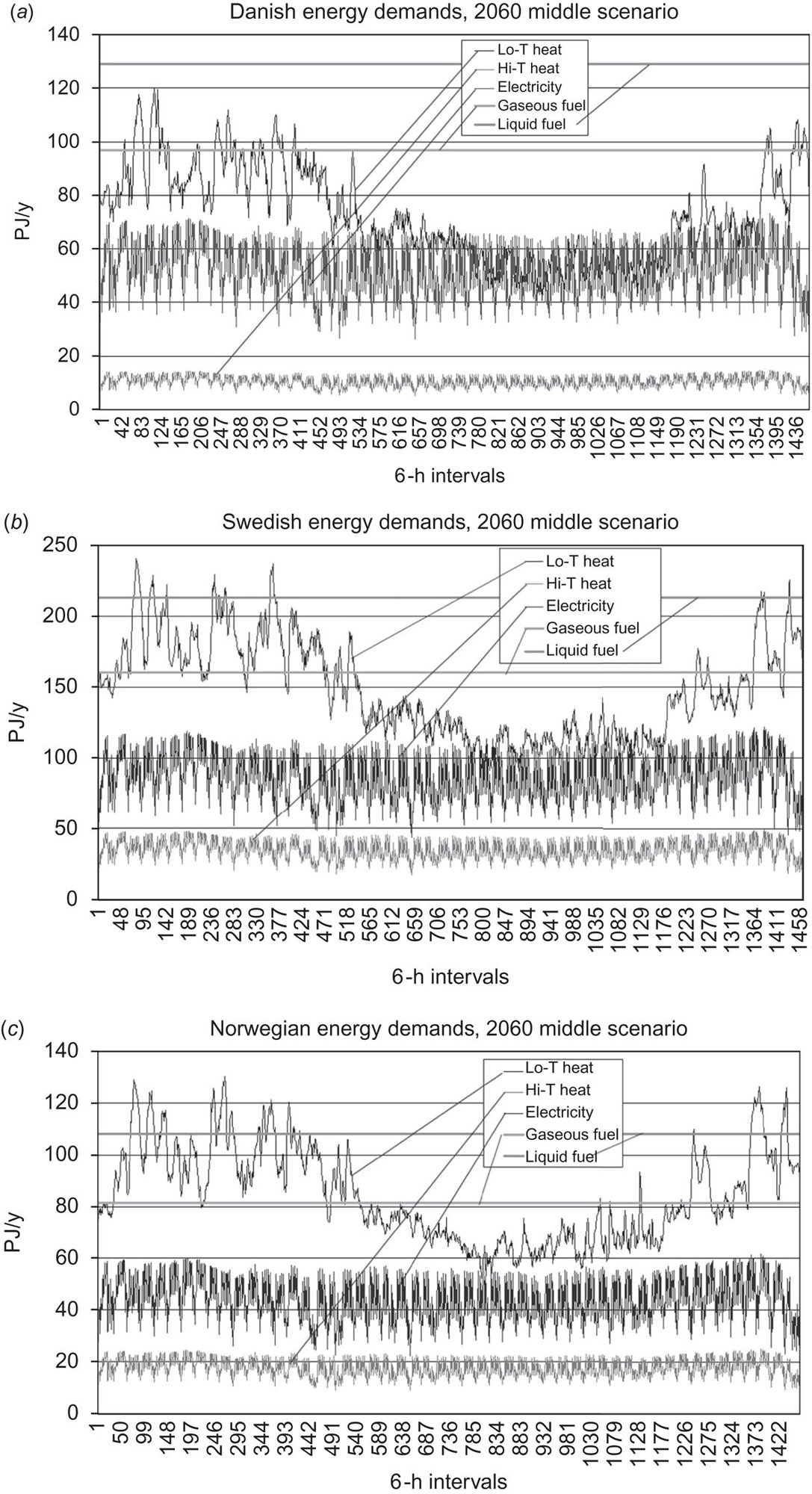
One purpose of the new study (Sørensen et al., 2008; Sørensen, 2008c) was to compare the alternative supply scenarios based on hydrogen and fuel cells, or on biofuels, as described in Sørensen (2008b). Here, the variant assuming that, in the transportation sector, liquid biofuels will be successful and hydrogen-fueled fuel cells will not is illustrated. Figure 6.87a–e show the 2060 energy demands for the five countries, according to the middle-efficiency scenario. Differences in the demand profiles reflect different climatic conditions and different industry structures in the countries.
In contrast to Denmark, other countries have substantial heavy industry demanding high-temperature heat and electricity, particularly in Norway. Despite its small size, Denmark has relatively higher transportation demands than the other countries, possibly reflecting the different industry structure. Space-heating needs show the expected dependence on degree-days of required heating of buildings.
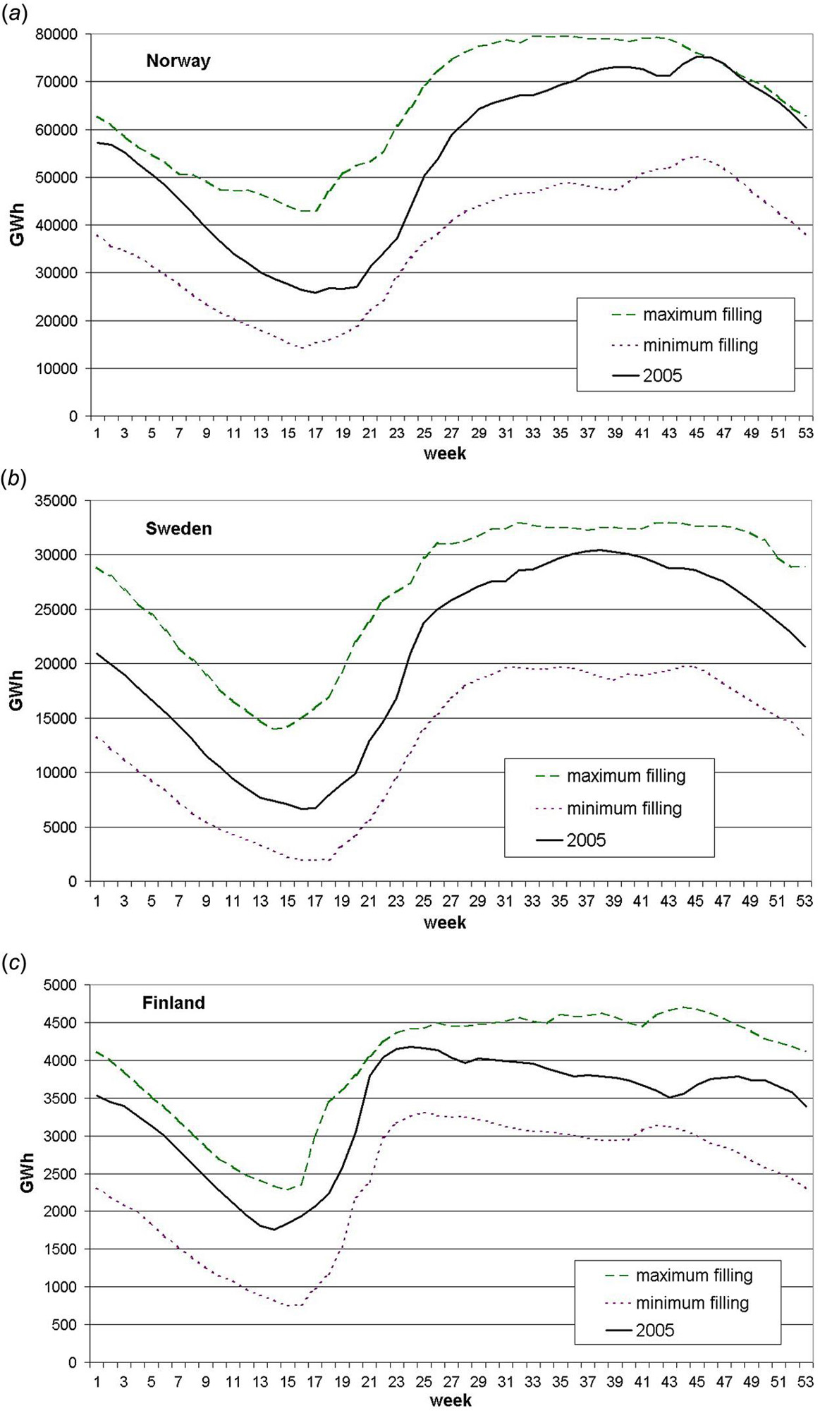
Generally speaking, the Northern European renewable energy supply options contain a very high percentage of electricity provision. This implies that high-temperature heat for industry would most conveniently be supplied by electricity, that low-temperature heat not derived from waste heat from other conversion processes would be supplied by electric heat pumps, and that electric vehicles are seen as an attractive option, if prices can be brought sufficiently down. Figure 6.88 (Nordel, 2005) indicates the options available in a system with hydropower based on large amounts of seasonal storage in the form of elevated water, which are predictable at the start of the season.

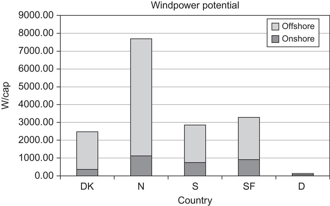
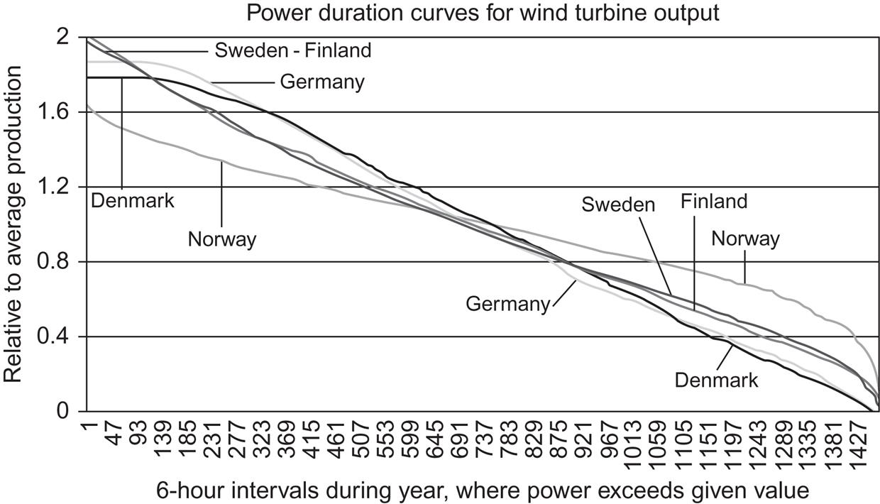
Wind conditions are excellent at nearly all locations near the Atlantic or Baltic coastlines. Figure 6.89 shows annual averages on a per capita basis. Relative to its size, the Danish wind potential is impressive, but the other Nordic countries, especially Norway, have large wind resources, notably offshore. On the other hand, several Norwegian offshore locations may be difficult to exploit (the criterion for inclusion in this study was a distance from the coast of less than 20 km, rather than a water-depth limit), primarily due to difficult conditions for transmission ashore and further to load centers. On the other hand, Norwegian winds are much more consistent than those of Sweden and Finland, and these are again more consistent than those in Denmark, as shown by the annual power duration curves in Fig. 6.90. The evaluation of the power duration curves assumes that the identified potential is fully used. It places turbines on 0.1% of the offshore areas closer than 20 km to the coast and on 0.01% of the inland areas (0.02% for Denmark, due to its lower fraction of inaccessible mountainous areas). In Norway, half the average power output is available more than 95% of the time, in Sweden and Finland, 85% of the time, and in Denmark and Germany, just under 80% of the time.
The Nordic countries can handle any remaining mismatch between supply and demand by using small amounts of the energy stored in the hydro reservoirs. Denmark could avoid using hydro stores situated in neighboring countries, should it wish to: The existing underground storage in caverns, presently used for natural gas, could store hydrogen produced from excess wind, and electricity could be regenerated when needed, using fuel cells or Carnot cycle power plants. As shown in Fig. 6.91, only a small store is required (less than the existing ones). Table 6.10 summarizes the renewable energy sources available in Northern Europe, for the assumed level of use. It should be noted that the biofuel potential is estimated on the basis of the Melillo model (see Fig. 3.99), which assumes that an optimum selection of trees and crops is planted, and that food, energy, and industrial uses of biomass is made sustainable by proper exploitation of grain, timber, and residues, including nutrient recycling considerations. For these reasons, the forestry estimate, for example, is about twice that of current productivity data for Sweden (Nilsson, 2006), estimated as concrete data for timber (updated in Swedish Forest Agency, 2012) supplemented with rough estimates for residues, but rather close to overall productivity data for Denmark, where agriculture plays a large role and forestry a small one.
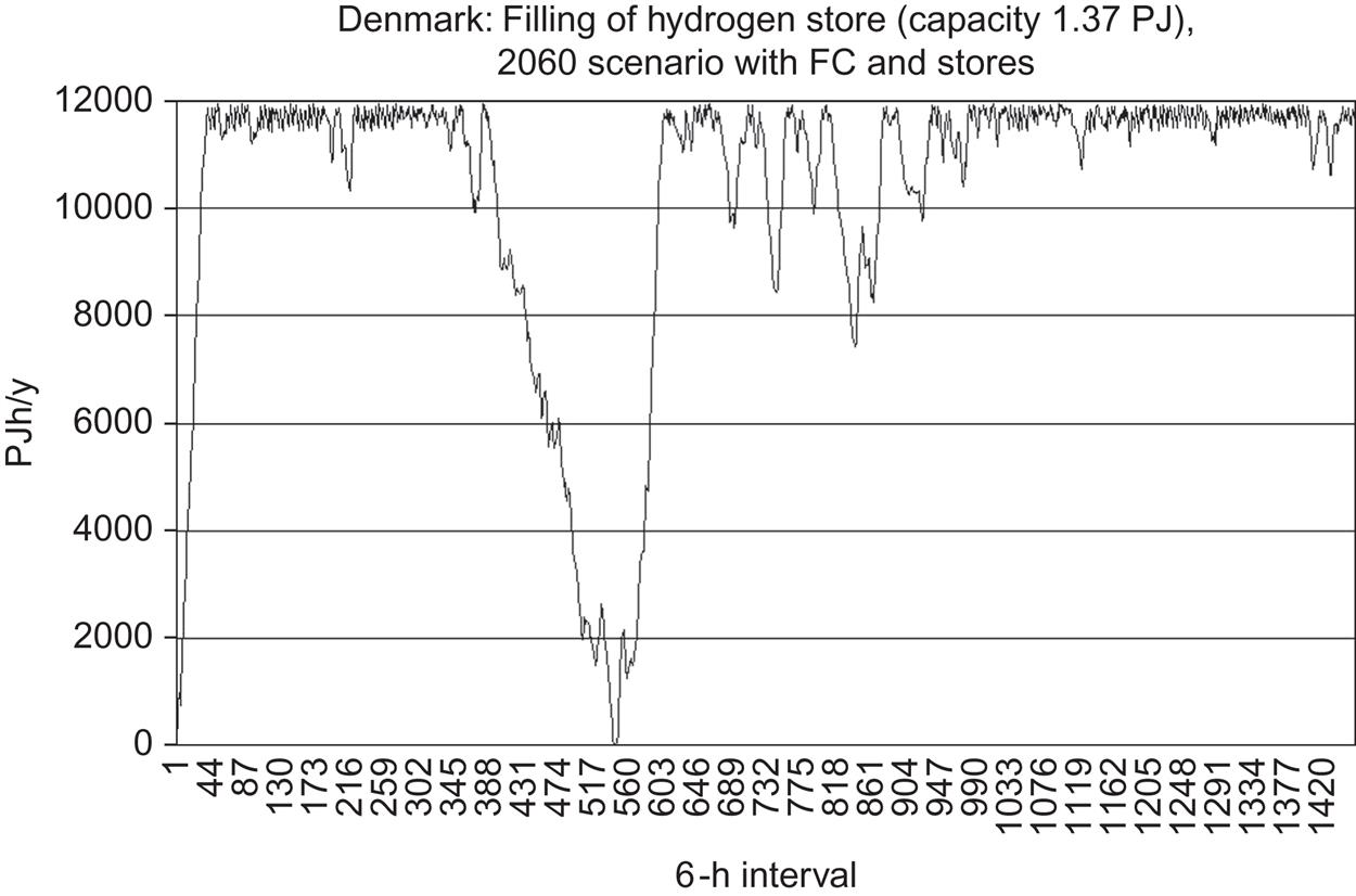
Table 6.10
Summary of potential renewable energy supply available for use in the Northern European countries considered (in PJ y−1). PVT is combined photovoltaic and thermal collectors.
| Country: | DK | N | S | SF | D |
| Wind onshore | 64 | 167 | 201 | 147 | 157 |
| Wind offshore | 358 | 974 | 579 | 391 | 177 |
| Biofuels from agriculture | 241 | 51 | 111 | 49 | 1993 |
| Biofuels from forestry | 58 | 523 | 1670 | 1180 | 892 |
| Biofuels from aquaculture | 153 | 223 | 320 | 205 | 108 |
| Hydro | – | 510 | 263 | 49 | 27 |
| Solar PVT electricity | – | – | – | – | 129 |
| Solar PVT heat | – | – | – | – | 275 |

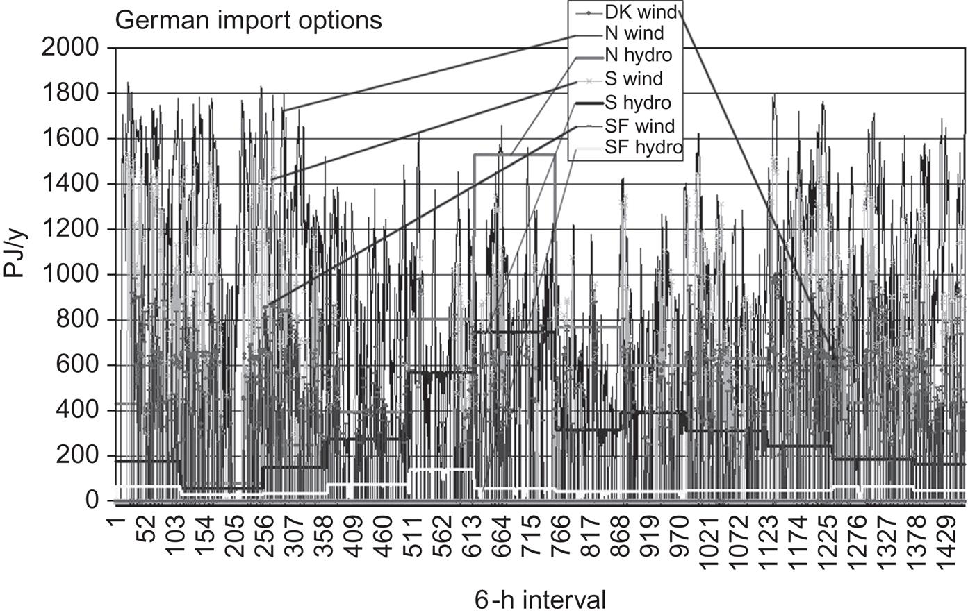
The year-2060 Nordic energy scenario first examines demand coverage in each country by indigenous resources, and then examines what potential remains for export. For all countries except Germany, full coverage of demands is possible without import (this does not say that economic optimization would not make it advantageous to trade more than strictly necessary).
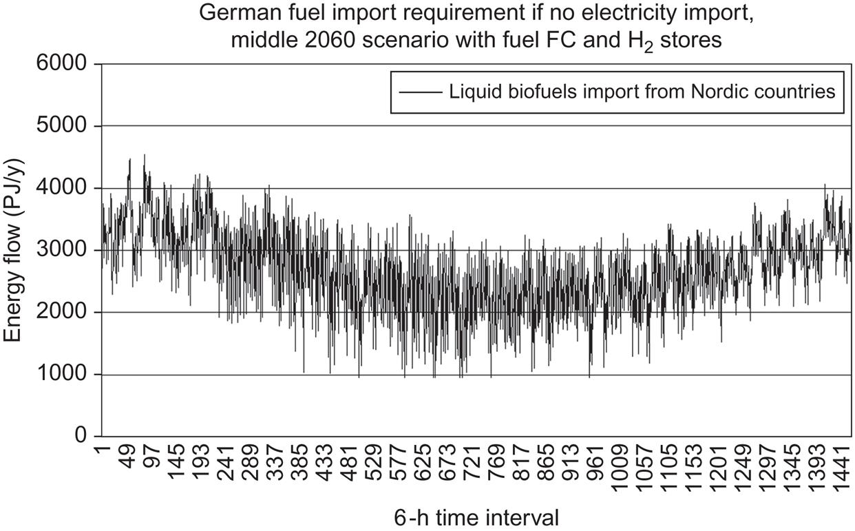
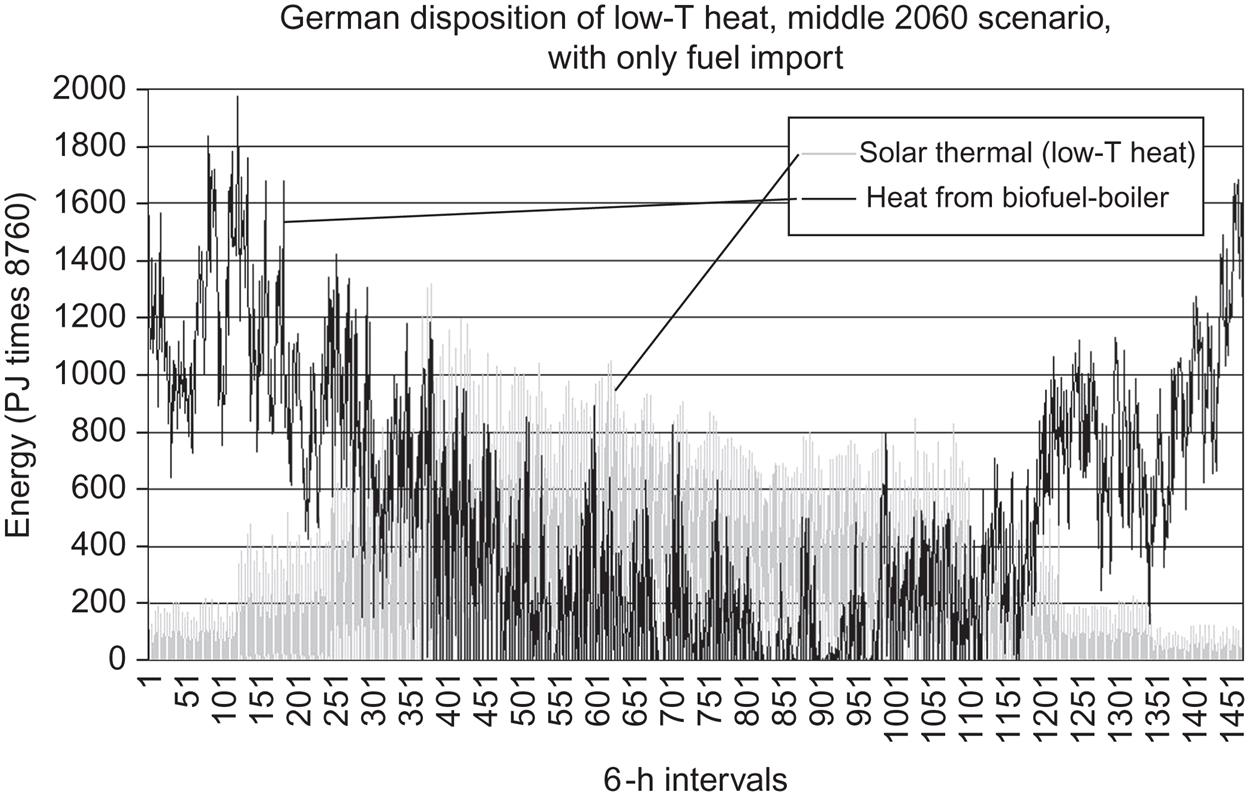
The import options available for Germany are depicted in the rather messy Fig. 6.92. There are total import options corresponding to more than twice the German requirement, so the mix of sources to import can be selected freely. A likely outcome would be to import any electricity needed for direct or industrial heat use and to let the transport sector import be determined by the relative success in developing second-generation biofuel vehicles, electric or hydrogen fuel-cell vehicles, or some hybrid between them. Figure 6.93 shows the German biofuel deficit as function of time. Of course, actual import need not follow this time pattern, because biofuels can be stored (e.g., at filling stations). Indigenously produced German biofuels suffice to satisfy heating needs in boilers, if this is the scenario chosen (Fig. 6.94). If the alternative high electricity import were selected, heating not provided by solar thermal collectors would be provided by heat pumps (details in Sørensen, 2008c).
6.6.3 Mediterranean region
The Mediterranean energy supply model presented here has been discussed in Sørensen (2011). Solar energy resources for the Northern Hemisphere are presented in Figs. 3.14 and 3.15, using 6-hour data for the year 2000. Based on the full 6-hour data, solar energy potentials for the Mediterranean region can be constructed, making the conversion process modeling described in section 4.4. In the Southern Hemisphere, appropriate tilt angles for solar collectors would be North-facing rather than South-facing. For those locations where measurements have been performed, the model seems to agree with data at mid-latitudes (i.e., the regions of interest here) and the variations in radiation seem to be generally of an acceptable magnitude. However, deviations could be expected at other latitudes or at locations with particular meteorological circumstances, due to the simplistic tilt-angle transformations.
Figures 6.87–6.95 gives an estimate of practical available solar energy potentials for the countries on the northern Mediterranean coast, and Fig. 6.96a and b gives similar estimates for the southern coast. For building-integrated use, it is assumed that an average of 4 m2 of collectors placed on roofs or facades of suitable orientation (close to South-facing and without other shadowing structures) would be available per capita. This area can provide solar power at an assumed photovoltaic panel efficiency of 15% and heat at an assumed 40% efficiency, allowing the same 4 m2 to serve both purposes. For centralized solar power plants, the available area is taken as 1% of the marginal land in the country. Population densities and land area uses are given in Figs. 6.1, 6.2, and 6.33–6.36. The centralized solar cell panels are placed in fixed horizontal arrays, which, according to the distributions underlying Figs. 3.14 and 3.15, work as well as tilted panels. However, if concentrators are used, it is necessary to add some amount of tracking. Furthermore, desert areas contained in several African Mediterranean countries provide such high levels of potential solar power that it is shown on a separate scale in Fig. 6.96b. This clearly constitutes a potential source for power export, if suitable transmission can be established.


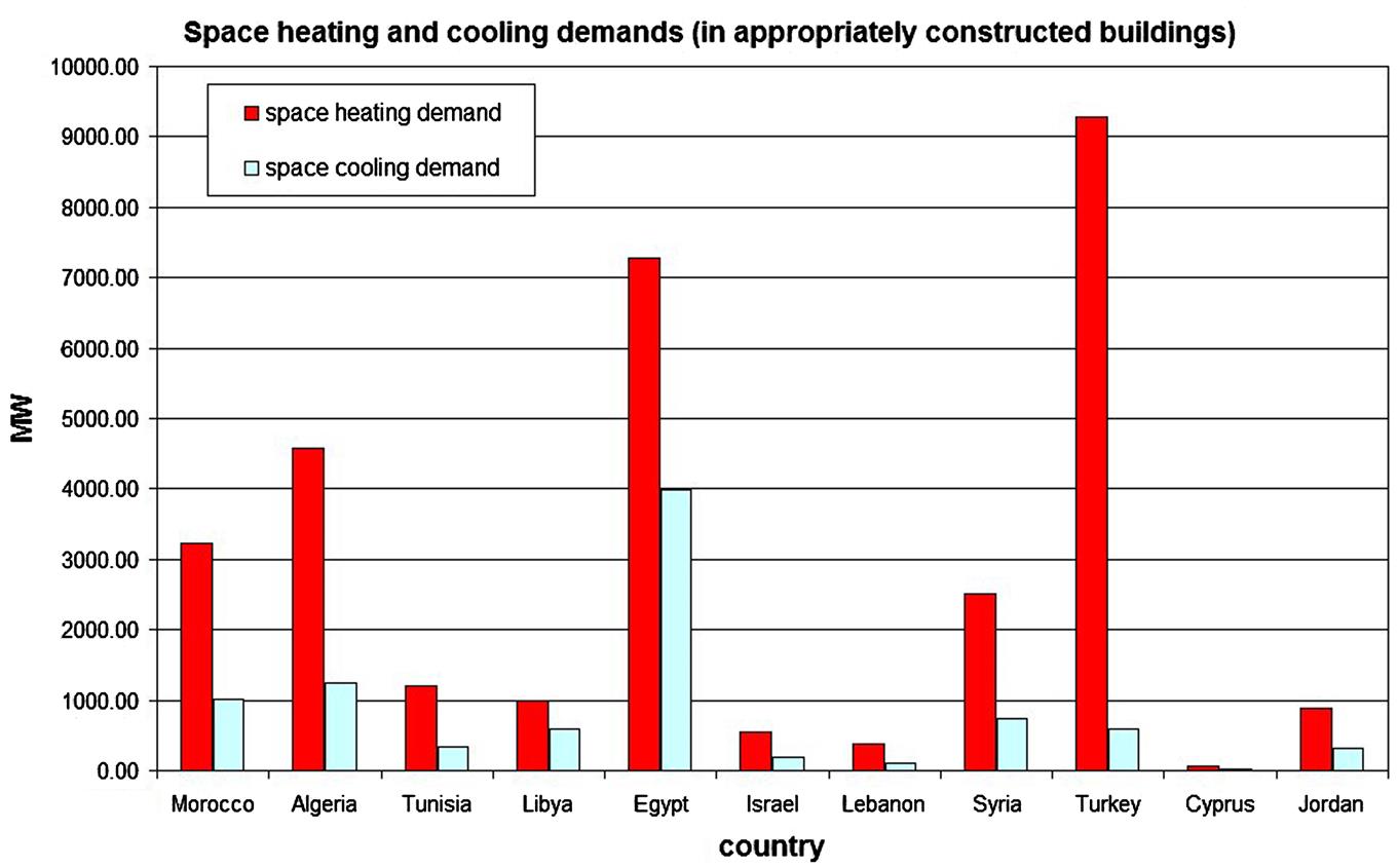
For comparison, Figs. 6.97 and 6.98 show the scenario heating and cooling demands in the same countries, using the methodology of section 6.2 and middle scenarios for consumption development (see further discussion below about the northern European scenario).

The temporal behavior of the 6-h time-series is illustrated in Figs. 6.99 and 6.100. In Fig. 6.99, the potential power production from building-integrated solar panels in Spain is compared to the demand for space cooling in properly designed buildings. Space cooling is assumed to be required if the temperature exceeds 24°C, as described in section 6.6.1. This fairly low energy expenditure for space cooling is valid for energy-efficient buildings (high insulation, controlled ventilation). Solar energy is well correlated with space cooling and the rooftop collection is more than sufficient for keeping the temperature below the limit selected.

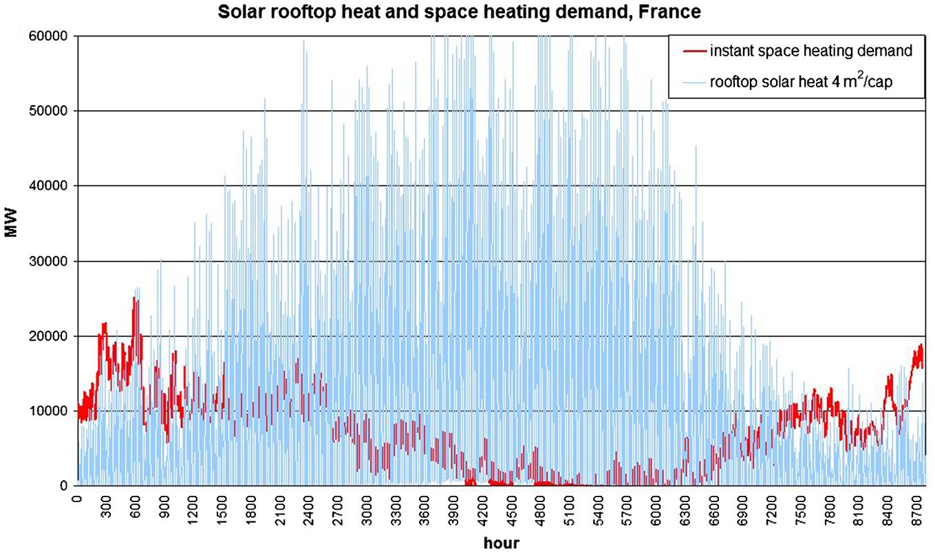
In Fig. 6.100, the thermal energy yield of 4 m2 cap−1 solar collectors in France is compared to the demands for space heating, again for energy-efficient buildings. The assumption is that space heating is required if the temperature is below 16°C, again with details given in section 6.6.1. Here there is an anti-correlation between solar energy collection and demand, and although the annually collectable solar energy is adequate, heat stores of several months of capacity must be added to make a solar heating system able to cover demand year-round. It should also be mentioned that the functioning of solar heat collectors depends sensitively on the temperature of the inlet fluid, and therefore there is an expected decreased efficiency in late summer and possibly a deficiency in temperature of the outlet fluid during winter, relative to the requirement of the heat-distribution system (worst for radiator heating, best for floor or air heating). During the summer months, additional heat collection for other uses than space heating is possible. Since the electricity production from the building-integrated solar PVT cells is assumed to be 15/40 of the heat production, it is clear that the rooftop solar collectors are far from capable of satisfying total power needs. The electricity that may be derived from solar panels on marginal land (Fig. 6.95) is insignificant in France, but in Spain, it could contribute to general electricity demands.
Wind resources could be used by decentralized placement of wind turbines on agricultural land, or more centralized placement on marginal land or offshore in fairly shallow waters that allow conventional foundation work (section 6.3.2). Figure 6.30 shows the potential wind-power production globally. The Mediterranean results are shown on a larger scale in Fig. 6.101. There are several areas of high potential, particularly in the eastern part of the region. Figure 6.102 shows the totals for each country along the northern Mediterranean shores, and Fig. 6.103 shows totals for the southern and eastern shores. It is assumed that 0.01% of the land area is suitable for wind production (representing the rotor-swept area and giving generous room for placing the turbines so that production is not lowered by interference between individual turbines), and that 0.1% of the sea area may be used without interference with other uses, such as fishing, shipping routes, or military training. Only areas with water depth below 20 m are considered.
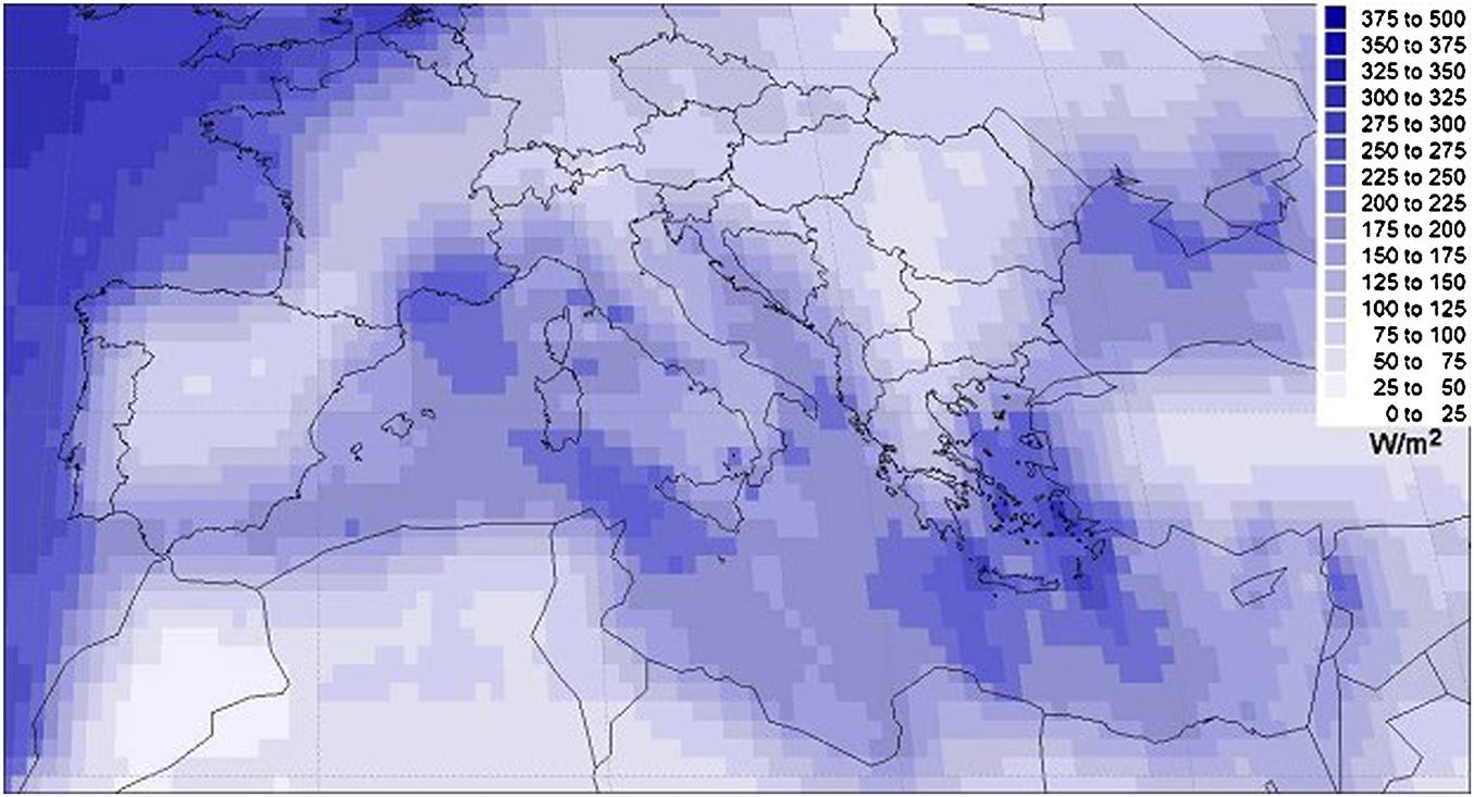
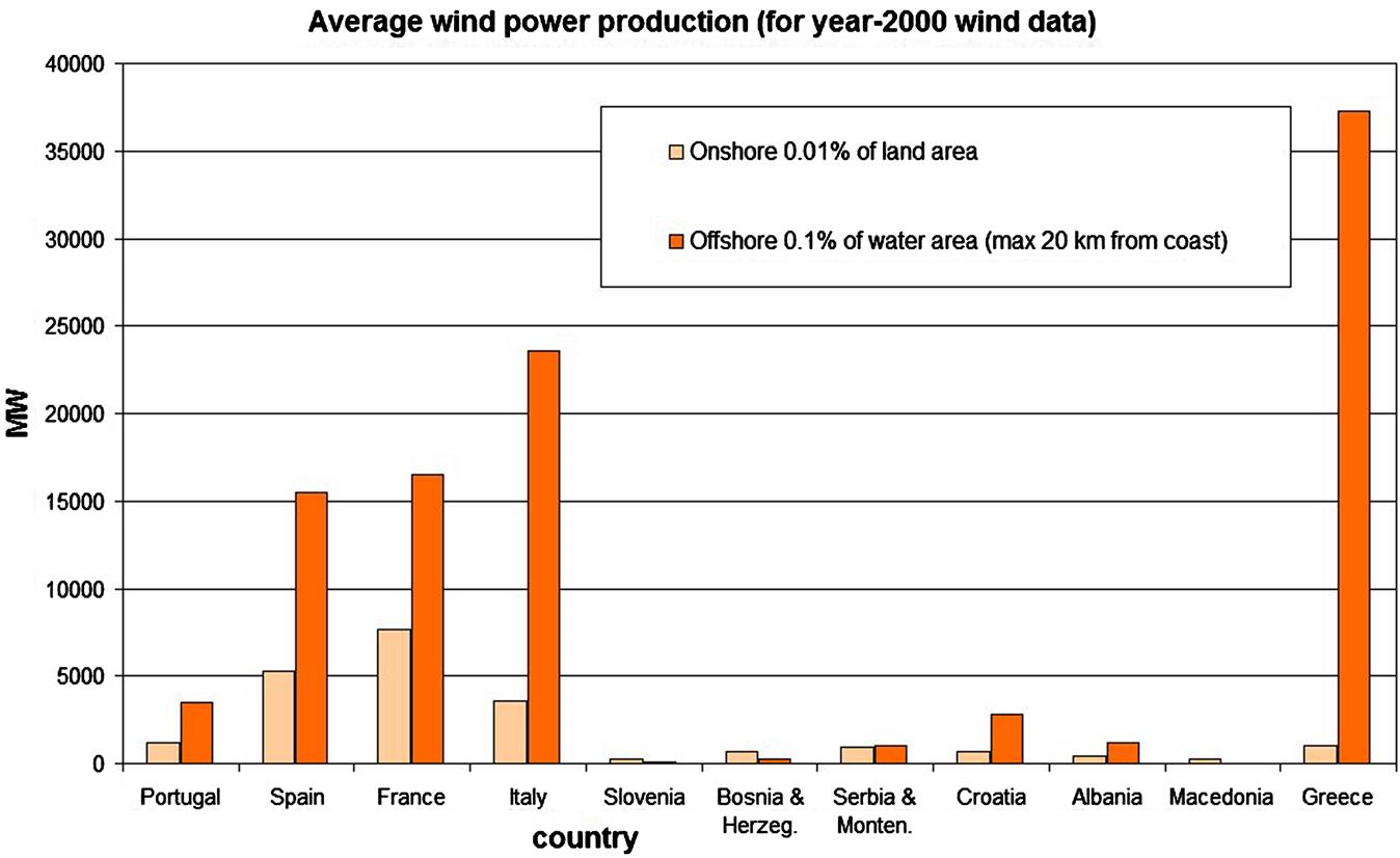

Countries near the Atlantic Ocean have substantial potentials, also inland, but in the eastern Mediterranean, Greece and the Turkish west coast are characterized by very large offshore potentials but little mainland onshore wind. This is illustrated by the time-series shown in Figs. 6.104a and b for Portugal and Greece. The combined wind potential for the total region is large enough to offer coverage of a substantial part of the electricity demand, together with smaller additions by photovoltaic power. The potential wind-power estimates are generally larger than the rooftop PV estimates, which should not be surprising, since wind farms on agricultural and marginal land are included. These locations also make the solar potential large, but it is restricted to areas without other uses, because solar cells cover the area while wind turbines have small footprints and allow agriculture on the same area.

The total renewable electricity production in the European Mediterranean countries (with the restricted assumptions on PV areas and number of wind sites, 0.01% of land area being actually less dense than the present penetration in Denmark) is not sufficient to cover the power demands of the middle scenario. However, the African Mediterranean countries have a huge surplus due to the potential of desert-located solar farms on just 1% of the land. This has caused several investigators to propose power exchange through one of the three cost-effective routes (Fig. 6.105). Political issues in some of the countries involved have so far prevented these ideas from being seriously pursued.

Biomass resources may be divided into resources associated with agricultural activity, with forestry, and with aquaculture. In each case, the primary products, such as food and timber, should get first priority. However, residues not used for these purposes can be used for a variety of other purposes, including energy. This has long been the case for simple combustion of biomass, but considerations of recycling nutrients to the soil or using biomass as industrial feedstock for a range of products may make it preferable to avoid simple burning, which has associated negative impacts from emissions to the atmosphere.
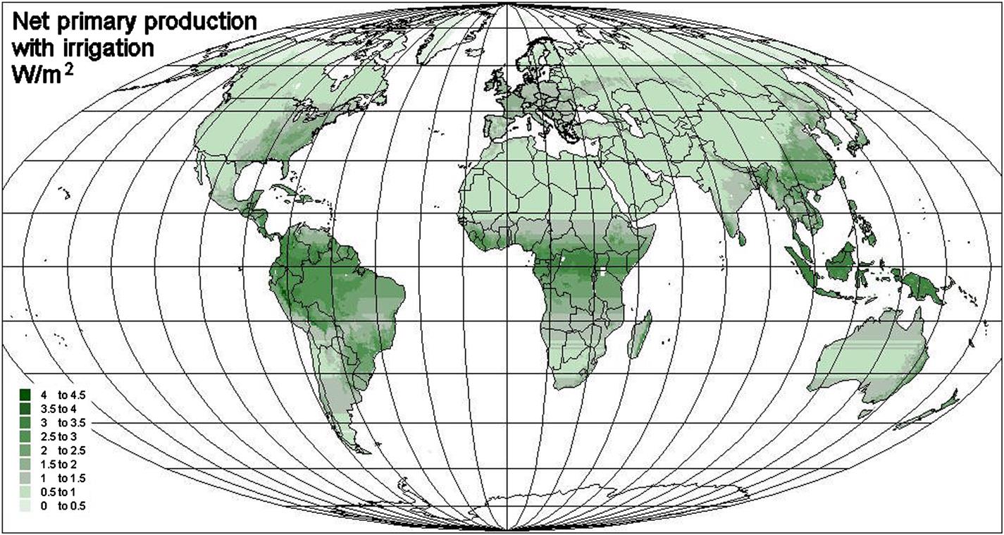
Biomass resources are estimated from the model of plant growth described in section 3.5.2, expressed as net primary production (NPP). The maximum amount of biomass that can be used sustainably for energy (as harvested crops, wood, etc., but recycling nutrients when possible), considering variations in solar radiation, precipitation, and nutrients as function of geographic location, is shown in Fig. 3.99. Figure 6.106 shows a variant where water is freely available and thus no longer a limiting factor. This gives the biomass production that would be possible with sufficient irrigation. Of course, it cannot be globally realized because many regions have water limitations that preclude full irrigation.
Based on the global models shown in Figs. 3.99 and 6.106, the annual biofuel potential in energy units is given in Figs. 6.107 and 6.108 for the Mediterranean region, with the following assumptions: Irrigation is not included, although some regions in the area considered presently use artificial addition of water, but nutrient recycling has been assumed, although it is not now fully practiced in the Mediterranean region (and administration of chemical fertilizer is used in some regions). Of the total primary production modeled, only half is taken as available for energy production. This means that, in the agricultural sector, considerably more than food is left to other uses (under 10% of the biomass energy yield ends up used as food, the rest being residues, such as straw or waste from processing and final use in households, all of which could theoretically be recycled to the fields). In forestry, 50% of NPP used for energy means that uses for timber, paper, and pulp are not affected, although sustainable wood usage would produce a similar amount of discarded wood products that could be recycled. The biofuel production efficiency is assumed to be 50% (of the raw material, hence 25% of the primary biomass produced), which is consistent with the 30%–50% efficiency expected for upcoming plants producing ethanol, methanol, biodiesel, or other fuels from biomass residues (the existing unsustainable use of food grains for producing biofuels in many cases has an efficiency greater than 50%).
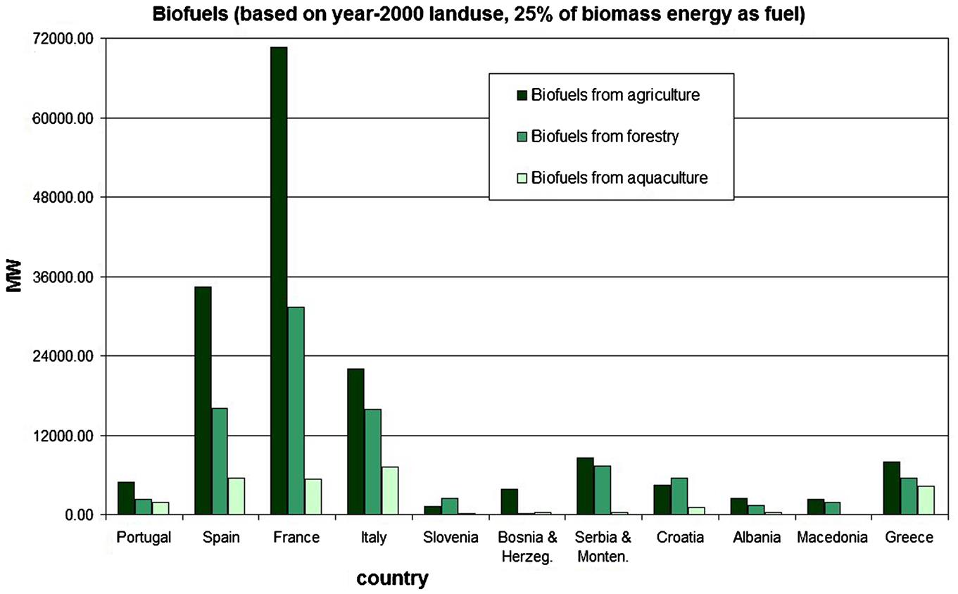

As shown in Fig. 6.107, France, particularly with its large food production (partially for export), has a similarly large energy potential for biofuels produced from agricultural waste, and Spain and Italy have a considerable potential as well. Some potential is also available in the Balkan region, and the same countries have an important potential derived from forestry residues. There is an amount of potential energy production from aquaculture, the largest being in Italy. The future will show how much of the potential water sites will be used for additional food production and how much for other aquaculture applications. The time variations in biomass supply are not particularly relevant, as biomass can be stored before or after conversion to fuels. As Fig. 6.108 shows, the soil is not amenable to large crop yields on the African side of the Mediterranean. Turkey, however, has substantial agricultural output.
It is likely that the future use of biomass residues for energy purposes will mainly be for fuels in the transportation sector. Here, biomass appears to be a considerably less expensive solution than battery- or fuel-cell-driven vehicles. However, combustion of biofuels still contributes to air pollution.
Other renewable energy sources that may play some role are geothermal energy; ocean currents, waves, and gradients in temperature or salinity; and, of course, hydro power, for which no more large installations are expected to achieve environmental acceptability, but for which there may still be a potential for smaller installations. The results can be used to construct full scenarios matching the renewable energy supply with expected future demands, and to identify the opportunities for trade of energy between the regions or countries. Such trade is very important because it can eliminate the need for energy storage to deal with the intermittency of some renewable energy sources, and because, as the preliminaries above show, there are areas in Europe that do not seem to have sufficient renewable energy sources domestically to support the level of population envisaged and their energy demands. An example of trade solutions (in the north of Europe) is treated in section 6.6.4. Here, basic supply–demand matching is carried out for one of the Mediterranean countries, Greece. The time-series of assumed demands, distributed on energy qualities, are depicted in Fig. 6.109.
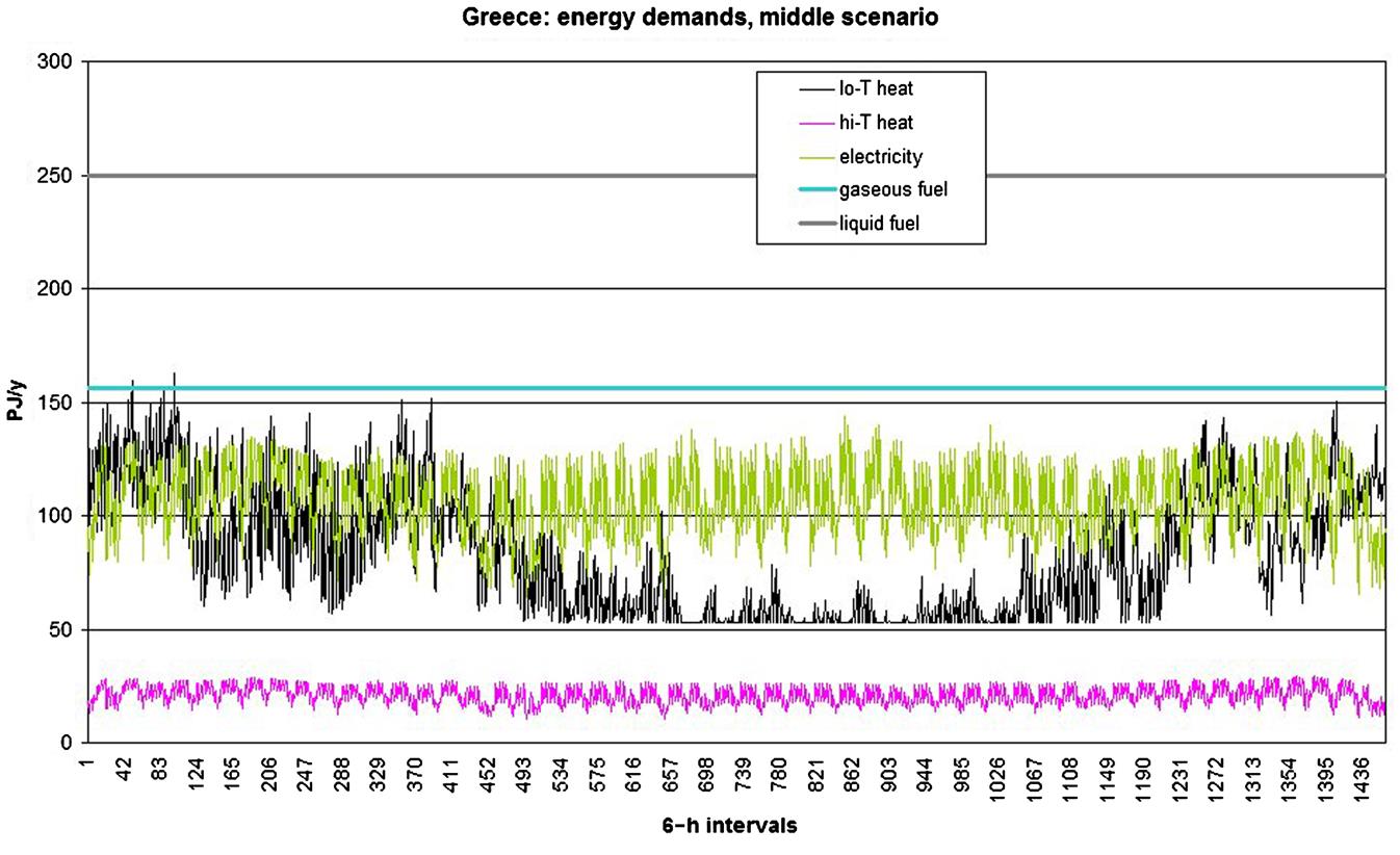
Figure 6.110 shows that a substantial part of the low-temperature heat demand can be covered by rooftop solar thermal collectors. The balance would be covered by heat pumps or by waste heat from building-size fuel cells, if they become viable by the scenario time, about 2050.
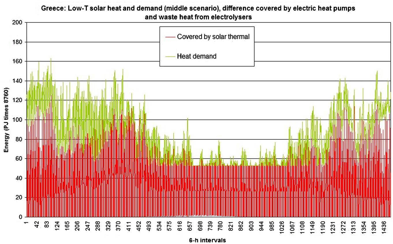
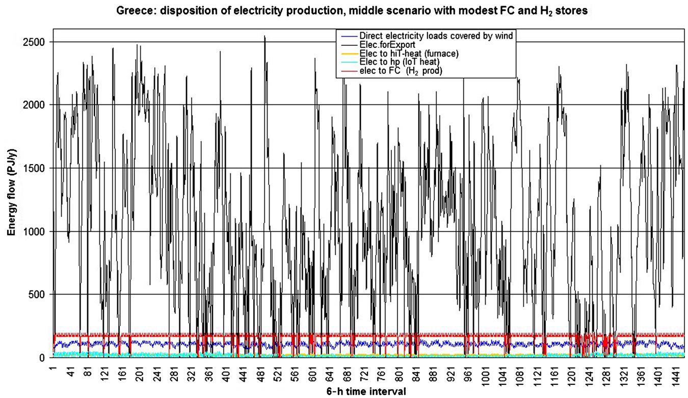
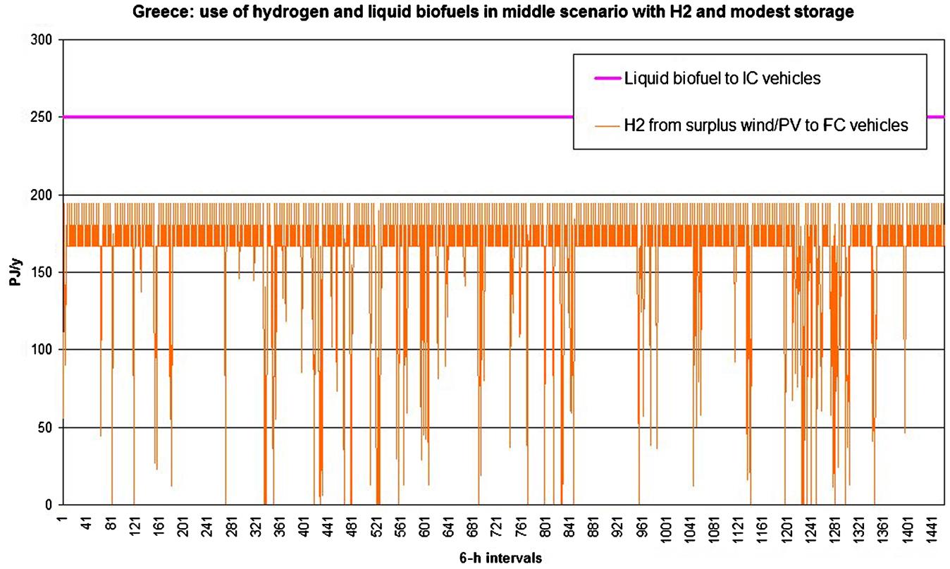
Figure 6.111 shows the scenario disposition of electricity produced by wind or photovoltaic cells. A fluctuating but quite large amount of power is available for export. Finally, Fig. 6.112 shows the coverage of transportation energy demand. Roughly half is covered by biofuels and the remaining by hydrogen in fuel-cell vehicles (more efficiency, hence lower energy demand). Only nominal hydrogen stores have been included in the model. They would have to be increased to avoid occasionally insufficient hydrogen production. The surplus power to feed the stores is available, as seen in Fig. 6.111.
6.6.4 North America
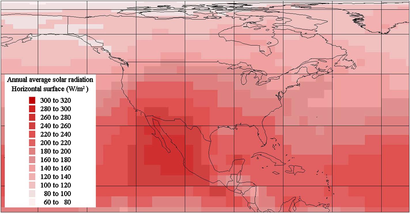
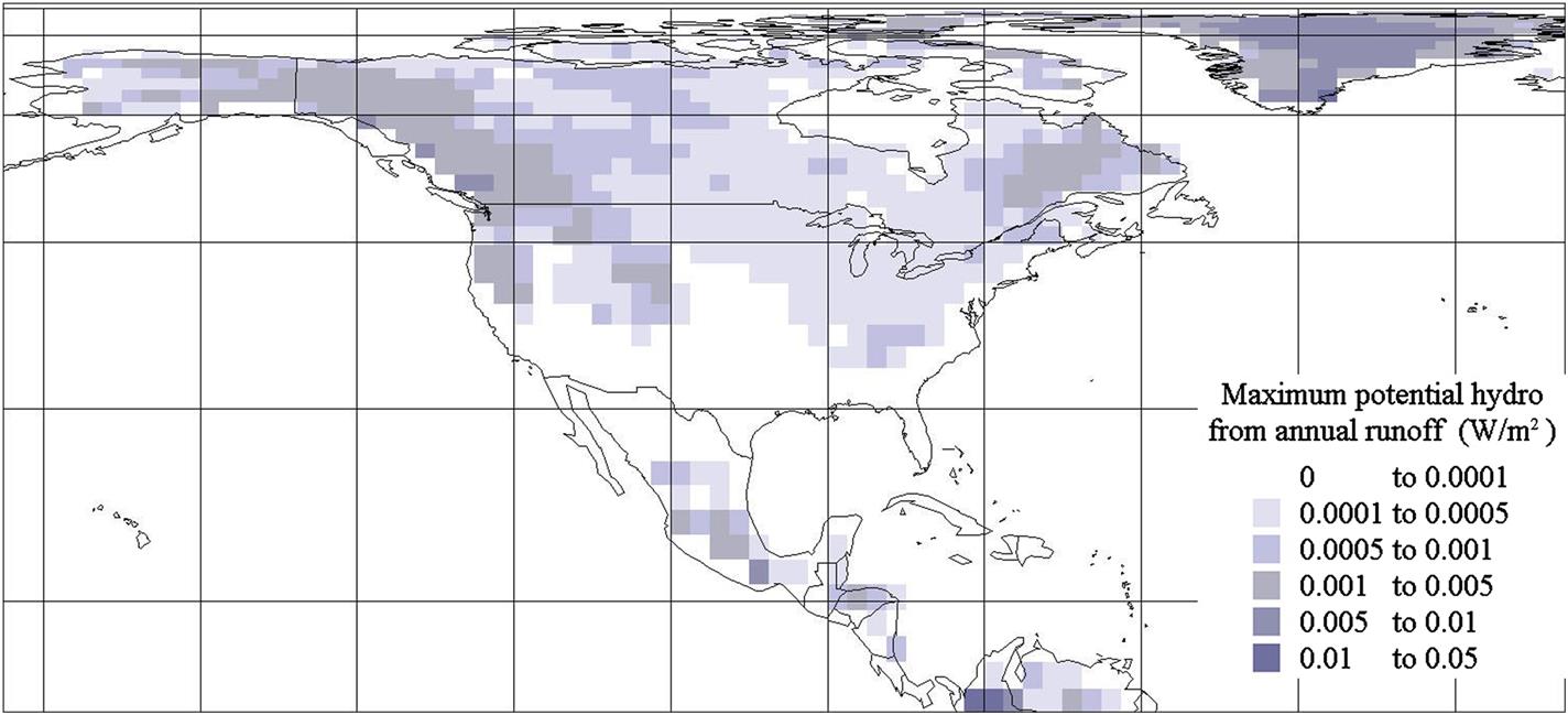
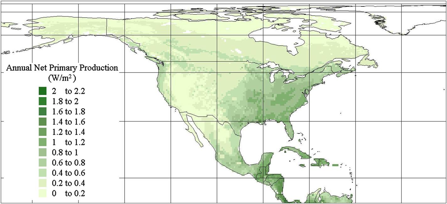
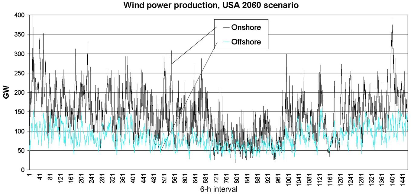
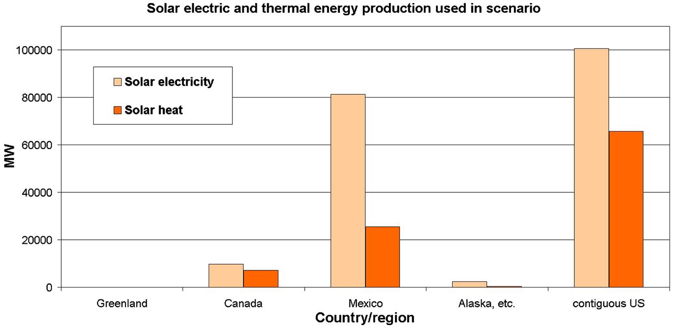
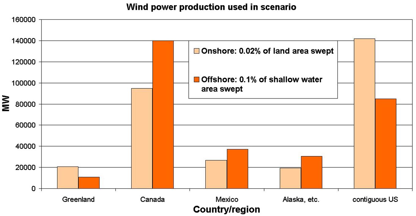
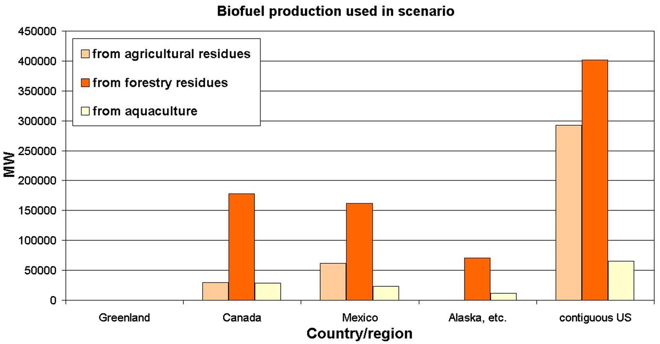
Major North American renewable energy resources can be derived from the material discussed in Chapters 3 and 6 (cf. Sørensen, 2007). Figure 6.113 shows the distribution of annual average solar radiation reaching a horizontal unit area, Fig. 6.114 similarly shows the potential average output per unit area of wind power produced by large turbines placed at safe separations in order to avoid interference. Figure 6.115 indicates possible average hydropower production, by combining run-off data with elevation above sea level. If the fall height between upper and lower reservoirs for practical reasons is only part of this, the available power estimate should be similarly reduced. Hydro utilization is largely assumed to stay at current level, and smaller sources, such as geothermal, wave, and tidal, are not included. Finally, Fig. 6.116 gives a measure of potential net average biomass production, using optimal crops and organic cultivation methods, but avoiding large-scale irrigation. If artificial irrigation is added, as it is to an extent today, the Midwest US potential is considerably increased. The potential for biomass utilization is largest in southern Mexico, the eastern United States, and a narrow coastal strip along the West Coast. An example of the time-development of onshore and offshore wind power production is shown in Fig. 6.117, for the contiguous United States, showing the common reduction of wind during the summer period. Figures 6.118–6.121 shows the parts of the total resources available for each of the four regions considered in North America (contiguous USA, Alaska and island communities such as Hawaii and Puerto Rico, Canada, Mexico, and Greenland) that is actually used in the 2060 energy scenario constructed. As expected, solar energy resources increase toward the south, biomass too with a similar but weaker latitude dependence and additional determinants such as precipitation and soil quality, hydro is largest in the North and confined to mountainous regions, and wind power largest in coastal regions or offshore. Some of the renewable resources could be utilized in much larger amounts than those suggested in Figs. 6.118–6.121, by assigning larger areas for solar collectors of wind farms, as the physical limit dictated, e.g., by shadowing effects of wind turbines placed too close to each other is still not close. The levels of renewable energy utilization suggested are rather determined by concerns of alternative area uses.


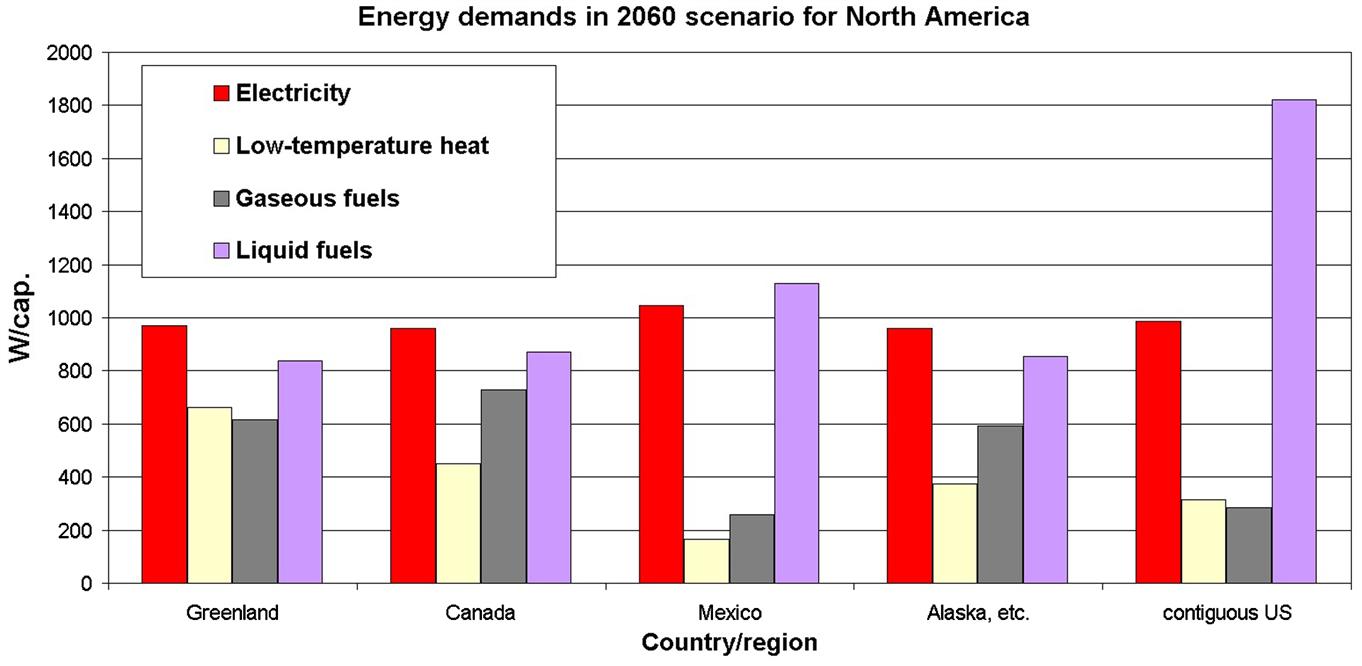
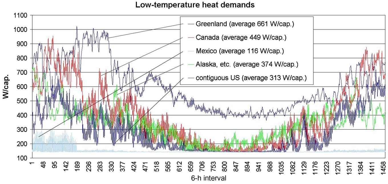
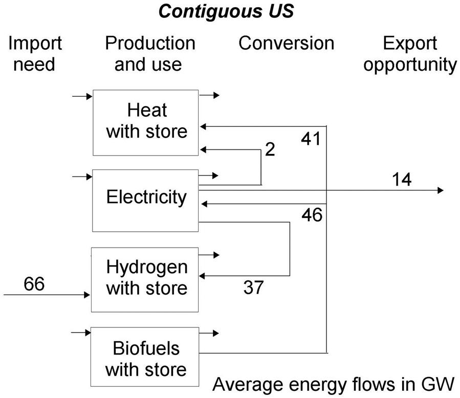
The aim is to explore the possibilities for a 100% renewable energy supply system in North America. It is suggested to look some years into the future, such as creating energy scenarios for 2060, in order that all current systems can be phased out at end-of-life rather than prematurely. Traditionally, North America has been characterized by low efficiency of energy conversion compared to, e.g., Western Europe, and it is generously assumed that even by 2060, the energy demands will still be about twice those indicated by the middle efficiency scenario of section 6.6.1. These demands are shown in Fig. 6.122, considering for simplicity only four energy qualities: electricity (assumed to be used for both dedicated demands and for high-temperature heat, as well as possibly for some lower-temperature heat by use of heat pumps), low-temperature heat (under 100°C), and gaseous and liquid fuels (such as hydrogen and biofuels). Figure 6.122 gives the annual averages of total demands, Fig. 6.123 gives the assumed time development of electricity demand, and Fig. 6.124 gives that of low-temperature heat demand with its substantial geographical dependence. The demands for gaseous and liquid transportation fuels depend on the detailed mix of technologies assumed used in the scenario for each region. For instance, the Mexico used more electric vehicles than the other regions (reflected in the otherwise similar electricity demand across regions), while the United States uses more liquid biofuels and Canada more gaseous (hydrogen) fuel cells than the United States and Mexico. The heat demand is based on temperatures for a particular year and is constructed using the assumptions regarding thermal building standards discussed above in section 6.6.1. Scenarios without doubling the demands have been explored by Sørensen (2015). Two scenarios have been constructed, using software simulation similar to that in the preceding sections, by either considering each of the four North American regions defined above as autonomous, or to allow trade and interchange of power and fuels between the countries/regions.

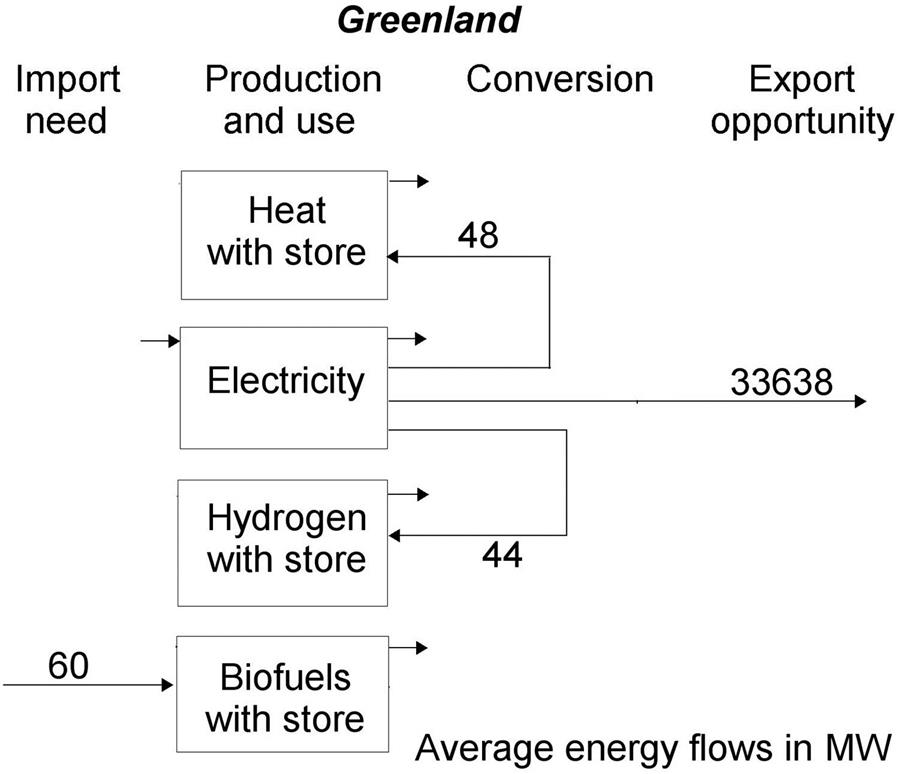
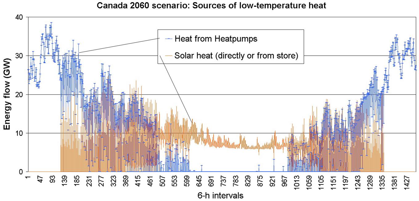
The overall results of the autonomous simulations are shown in Figs. 6.125–6.129, showing any supply-demand mismatch and an import requirement or an export option for each of the four energy forms considered. Due to the intermittency of some of the renewable source flows, energy stores are included as well as conversion between energy forms needed both for storage and retrieval, and for providing the demanded energy form from the running harvests of different renewable energy types. The United States is unable to produce enough hydrogen for its transportation sector (despite the shift of demands to biofuels assumed) and thus has an import requirement. In this high-demand scenario, Mexico needs to import both electricity and hydrogen, but since electricity may be converted to hydrogen before or after transmission to Mexico, the choice depends on the relative cost of electric transmission lines and hydrogen pipelines. It is seen that Alaska and Canada have large export potentials for both electricity and biofuels, while Greenland has only electricity to offer. However, all of these opportunities can be realized only by establishing power line connections or fuel transport routes, and depending on demand structures, a need for conversions between energy forms may also be required. In the concrete scenarios described below that are considering interchange between the regions, the fuel exchange may be of pipeline hydrogen, which is a clean fuel, or of liquid biofuels, if the transportation sector can be made to use these in an environmentally acceptable way. If not, the biomass residues should be used for hydrogen production rather than for production of liquid biofuels. As regards coverage of low-temperature heating needs, the thermal energy co-produced with electricity in PVT building-integrated solar panels or produced in communal solar arrays, with local storage options, suffices at lower latitudes, but at higher latitudes only during a period in summer, as seen from the Canadian simulation results shown in Fig. 6.130. During spring and autumn, there is some solar contribution, but most heating is provided by electricity through heat pumps. In winter, the solar panel thermal circulation is shut down due to risk of frost damage, and the heat pumps deliver all heat required. Any required cooling is provided by electricity-powered devices. The scenario has additional PV installations on marginal land, but using at most about 1% of such areas (Fig. 6.36).

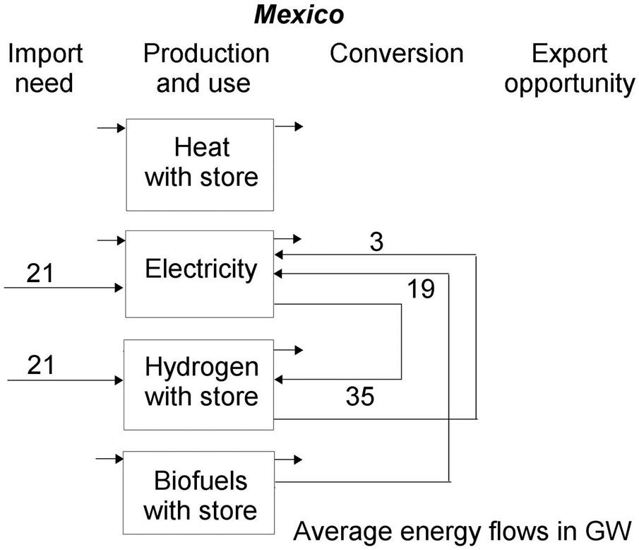
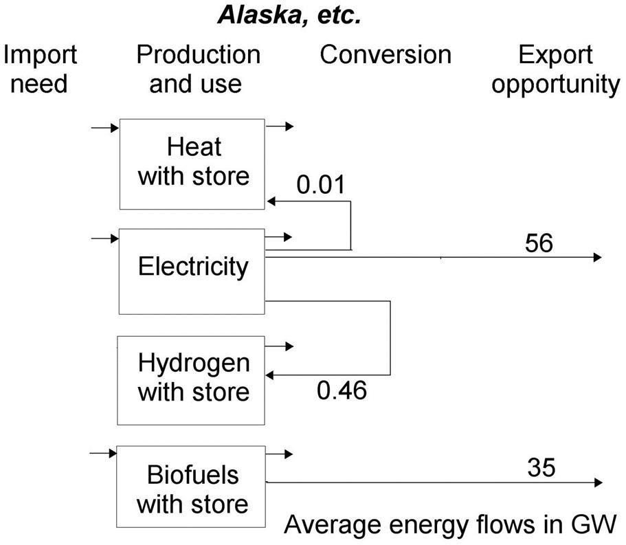
A second set of simulations was carried through with consideration of energy import and export between the North American regions considered, again using a computer model (called NESO) with 6-hourly time-steps (conforming with the available spacing of wind data) and some rules for the priority of indirect ways of satisfying a given energy demand with the renewable energy production available in that given hour, through conversions, drawing on stores or imports. Because of the time variations in need for import and surplus for export can be quite substantial, the addition of exchange options may to an extent change the behavior of the supply systems, relative to the outcome of the simulation treating each region as autonomous. The simulation of the connected regions will determine the amount of transfer capacity required, in interplay with the amount of energy storage in the system. Thus, there will not be a single “best” solution, but a choice between reliance on storage and transmission technologies, the cost of which have quite many components depending on local conditions and the precise technologies employed. For example, if conversion to and from hydrogen is used to store electricity, the cheapest hydrogen storage facilities are in cavities established in aquifers or salt domes (the cost estimated as 2.4 M$ per PJ storage capacity; Sørensen, 2012), but these are not necessarily available everywhere, and in case regeneration of electric power from hydrogen is required, the power plants doing this should preferably be placed near the hydrogen stores. There are also competing transmission technologies, both for power and hydrogen gas transport. Overhead lines may not be acceptable for environmental reasons (in populated or recreational areas), so the more expensive underground cables would have to be used.
Electricity import is required for Mexico* and the closest location of sufficient surplus is Canada. Rather than transmitting power between these distant locations, there would be exchange between Canada and the United States and between the United States and Mexico, finding the shortest transmission distance with consideration of the management of other loads in the regions passed through. Since both the United States and Mexico also has a need for hydrogen import (despite the emphasis on liquid fuels in the transportation sector chosen), additional electric power from Canada may be invoked for transformation to hydrogen. This conversion would take place at the end-point after transmission, if hydrogen pipeline transport remains more expensive than power line transmission. The simulation results (Sørensen, 2015) for the time-dependence of the maximum Canadian export opportunities and for the actual Canada-to-United States and the United States-to-Mexico power transmissions used in the scenario are shown in Figs. 6.131–6.133. The availability of power for southward transmission varies substantially and sometimes it is negative, signaling a need to transmit power in the northward direction. This is due to occasional lack of surplus in the Canadian system, typically at times of low wind, while high wind is the main cause of the occasional large surpluses. The variations could be diminished if more Canadian hydro was used for domestic supply during low-wind periods and correspondingly less hydro in periods of wind energy surplus. In this way, the overall functioning of the hydro reservoirs would not be affected (similar to the situation for Norway in the North-European model described above). Further control of fluctuations can be achieved at the receiving end, by varying US and Mexican hydrogen production according to the availability of power import rather than being constant over the year. Making use of Canadian hydro to smooth the import requirement would further allow the transmission capacity to be lowered, both from Canada to the United States and from the United States to Mexico. The Canadian hydro production assumed in the model (37 GW on average) is not expanded relative to the current one and is insufficient for totally flattening the power export over time.


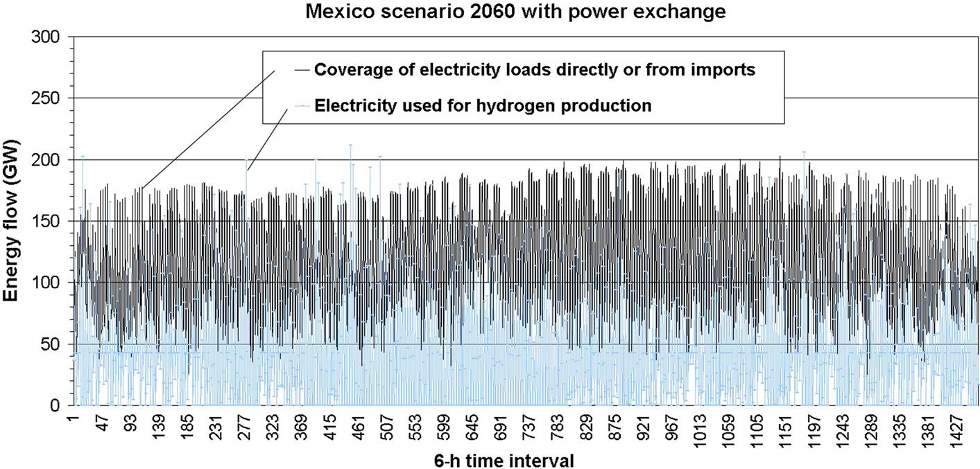
Figure 6.134 shows how the Mexican electricity demand is met by a mixture of indigenously produced and imported power, and how the additional hydrogen required by the transportation sector is produced with a rapid time variations, dictated by the availability of wind and photovoltaic power and the demand variations (such as day-to-night, weekday-to-weekend). Figure 6.135 shows the dramatic time variations in the amounts of hydrogen stored in Mexico, due to the variability in production. A storage capacity of at least 1000 GWh is included in the scenario, in order not to fail to meet vehicle hydrogen demands. The liquid fuel use also shown is taken as constant, because storage of liquid biofuels is inexpensive and similar to the setup at current gasoline stations.

Quoted costs of large-scale electric transmission vary from around 0.5 M US$/km for a 700 MW landline to 1.4 M US$/km for a 3 GW landline (Niederprüm and Pickhardt, 2002; Silverstein, 2011). For the European 500 km sea cables between Norway and the Netherlands or Germany, quoted costs are from 0.5 to 1.0 M€/km for a capacity of 700 MW, and some 1.2–2.7 M€/km for 1400 MW capacity (Alegría et al., 2009; Chatzivasileiadis et al., 2013). Overhead landlines used to be at least five times less expensive than sea cables, but increasing environmental and popular concerns has in many regions banned overhead lines in populated or recreational areas, using buried coaxial cables instead, which has made the onshore and offshore costs more similar. The undersea cables are typically carrying high-voltage direct current with transformers at each end. Current losses are mostly under 4% and losses below 2% are possible for new lines (Pickard, 2013). The scenarios considered here in several cases have a choice between electricity and hydrogen transport. Hydrogen pipelines have to be built to higher standards than most of the natural gas pipelines currently in operation, which is estimated to add some 25% to cost (Sørensen et al., 2001; Beaufumé et al., 2013). This makes the current estimated cost of GW hydrogen pipelines lie somewhere between the cost of landline and sea cable electricity transmission costs, at 1.0–1.5 M US$/km (Gondal and Sahir, 2012; Johnson and Ogden, 2012).
Figure 6.136 shows the overall picture of the North American 2060 scenario with electricity transmission used to eliminate supply-demand mismatches in conjunction with local electricity-to-hydrogen conversion and hydrogen stores, typically located close to the conversion facilities. It follows from Figs. 6.132 and 6.133 that the capacity of power transmission lines between Canada and the United States should be near 400 GW and that between the United States and Mexico near 350 GW, due to the high requirements in the last part of the year. These lines carry quite substantial costs, especially for those segments that may require underground cables.

6.6.5 Japan and South Korea
For Japan, South Korea, and China, the high population densities pose severe challenges to an all-renewable energy system. For this reason, a more detailed and hopefully more accurate model has been used in simulating scenario behavior similar to the ones for Europe and North America. For estimating the very important offshore wind potential, the simple model of just including model grid units with both land and ocean fractions was replaced by a more refined model, considering the actual depth to the sea floor and calculating the potential for turbines accepting up to 20 m and up to 50 m foundation depths (20 m being characteristic of most existing offshore wind parks and 50 m being the maximum considered feasible with current technology). Also the solar model was improved, by replacing the sine-variation-with-stochastic-overlays model used for Europe (Sørensen, 2008c) and North America (above) by the model based on actual horizontal radiation data described in connection with Figs. 3.14 and 3.15. Here, about two-thirds of the radiation is considered to come from the direction to the Sun or close to it (and thus easy by geometrical means to transform to the inclined surfaces assumed for solar collectors), and the remaining scattered radiation is assumed to be more evenly distributed, either isotropic or according to the Kondratyev and Fedorova (1976) model described in Chapter 3. For Japan and South Korea, the smaller physical size of the countries allows the fairly coarse 2.5°×2.5° satellite data resolution for solar energy used for North America (Fig. 6.113) to be refined to a grid size of 0.125°×0.125°, even better than that of the scatterometer wind data (0.5°×0.5°, cf. section 6.3.2).
The main renewable energy resources available in the East Asian region are shown in Figs. 6.137–6.140, as time averages over a typical year or for a summer and a winter month in the case of solar radiation. The scenarios described below for Japan, South Korea, and China uses only a part of these resources, for a variety of reasons that will be discussed. Scenarios for Japan and South Korea, with the possibility of energy trade between them, have been explored by simulation in Sørensen (2015, 2017), and these calculations form the basis of the overview given here. The scenario in the 2015 book is characterized by high wind power usage, while that in the 2017 article has a high solar energy contribution and fewer onshore wind turbines.


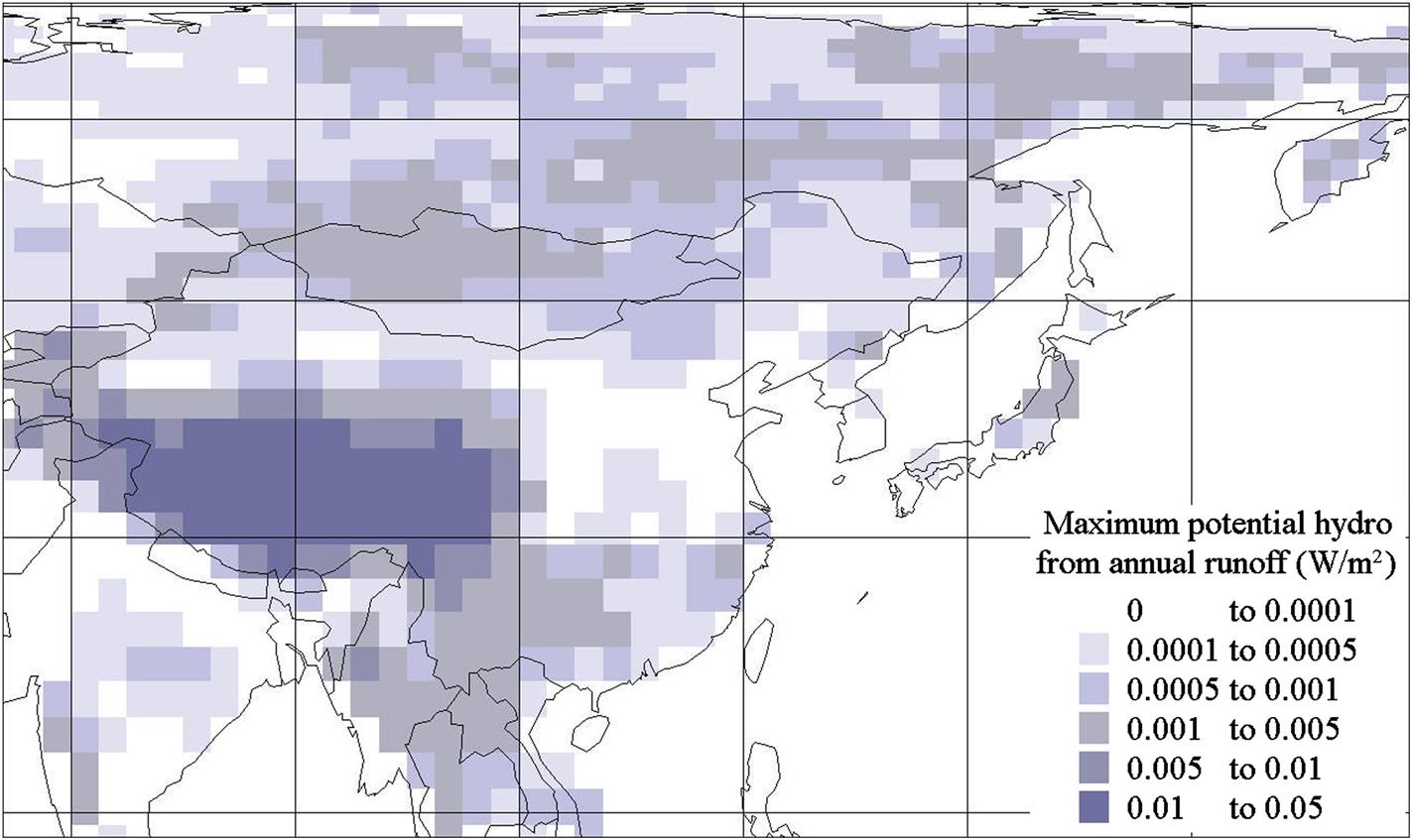
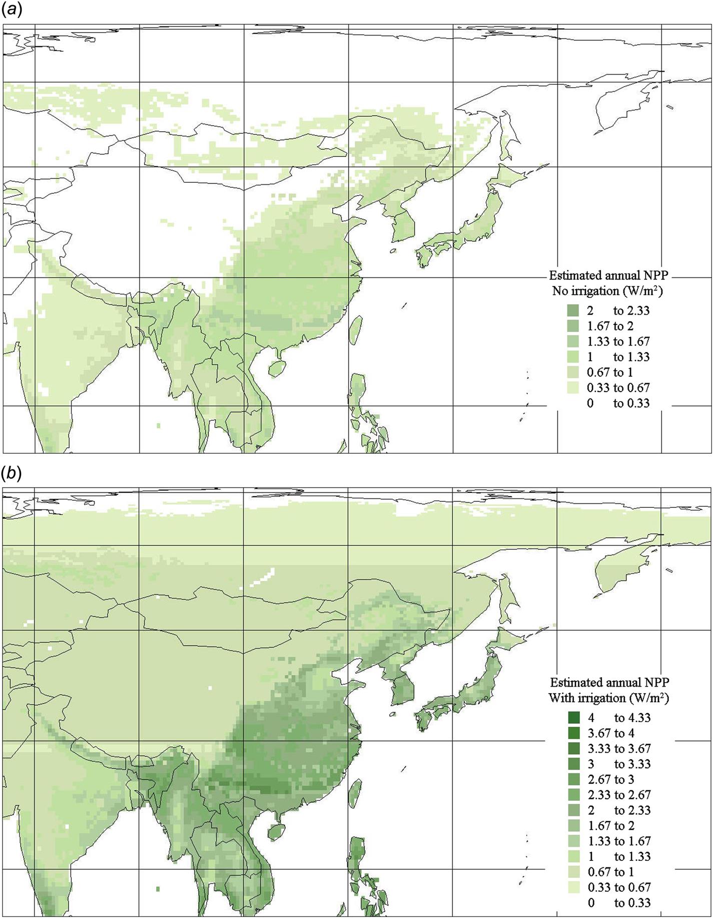
Due to high frequency of cloudiness, Japan receives less solar energy per square meter than South Korea (see Fig. 6.137b), but still amounts quite adequate for photovoltaics and preferably co-produced solar heat. However, the marginal land areas where centralized solar arrays could be placed are rather scarce in both Japan and South Korea, and building surfaces or roofs also offer less opportunities than in Europe or the United States, due to a lower dwelling area per capita and due to many high-rise buildings or buildings shadowing each other. It is therefore a very aggressive use of solar energy when the recent 2050 scenario (Sørensen, 2017) derives an average 25 GW of electric power and 18 GW of low-temperature heat from solar devices in Japan and 12 GW power and 5 GW thermal energy in South Korea. Even at a PV panel conversion efficiency of 20%, this would require some 5.7 m2 of collector area per capita in both Japan and South Korea (assumed 2050 population 110 M and 52 M), somehow divided between building-integrated and freestanding collectors.
Wind conditions in Japan and South Korea are excellent for power production, both onshore and offshore, although the Japanese sea floor drops rather quickly, making the 50 m foundation limit assumed here restricts the resource to a rather narrow band near the cost, as shown in Fig. 6.141. For Japan, the scenario uses 22.4 GW wind power offshore and 50 GW onshore, where the latter could be increased by some 30% without impacting on recreational land areas. For South Korea, the scenario uses 20 GW wind power offshore and 14 GW onshore, taking advantage of the larger distance of the 50-m depth line from the shore at the country’s west coast to spare some of the very few marginal land areas onshore.

There is some hydropower currently produced in Japan but little in South Korea. These plants are continued without expansion. Biofuels are available in both countries, from agricultural residues and from aquaculture, while residues from forestry are substantially large in South Korea than in Japan. The aim is to satisfy a substantial part of the transportation energy demands by biofuels, but in Japan, hydrogen produced by excess electricity needs to cover as much as 50% of the transportation energy demand.
Energy demands assumed for Japan and South Korea include service demands 2.5 times higher than the present ones for electricity, folded with a factor four increase in efficiency, in line with the remarks made in section 6.2 regarding the relative cost of efficiency improvements relative to supply-system expansions (Fig. 6.142). No further doubling of power demands like in the North American scenarios is made, because efficiency is an established virtue in the South-East Asia region. Heating and cooling needs are modest with the assumption that the building stock by 2050 is reflecting the best energy-efficiency standards known today. Public transportation already today plays a large role and helps to satisfy mobility needs in an energy-efficient way, and the assumed transportation energy demand of 600 W per capita (based on more than doubling activity, folded with over two times current average efficiency) may well be too high, considering the likely efficiency development of battery, hydrogen, and biofuel vehicles and the economic limit to how much time can profitably be spent on relocating goods and people. While the scenario considers large quantities of energy converted from electricity to hydrogen for use in the transportation sector, the actual pattern may as well be a mixture of fuel cell vehicles and electric vehicles, or rather hybrids between the two. No attempt has been made to guess the relative shares of fuel cell and battery traction, as it makes little difference for the overall scenario, because the energy in both cases comes from electricity and at fairly similar conversion efficiencies. At present, the efficiency of charging batteries and delivering traction energy to wheels by an electric motor is higher than the efficiency of hydrogen production by electrolysis and subsequent fuel cell operation, but the gap may narrow with time. Therefore, the scenario assumptions are in this case reflecting a “worst case.” A serious obstacle to both electric and hydrogen vehicles is the short lifetime (typically under 5 years) of both batteries and fuel cells, as compared with increasing vehicle lifetimes (currently approaching 20 years). Three replacements of these currently very expensive parts of the vehicle will make a large negative economic impact, relative to biofuel vehicles, even if environmental externalities are included for the biofuel combustion.
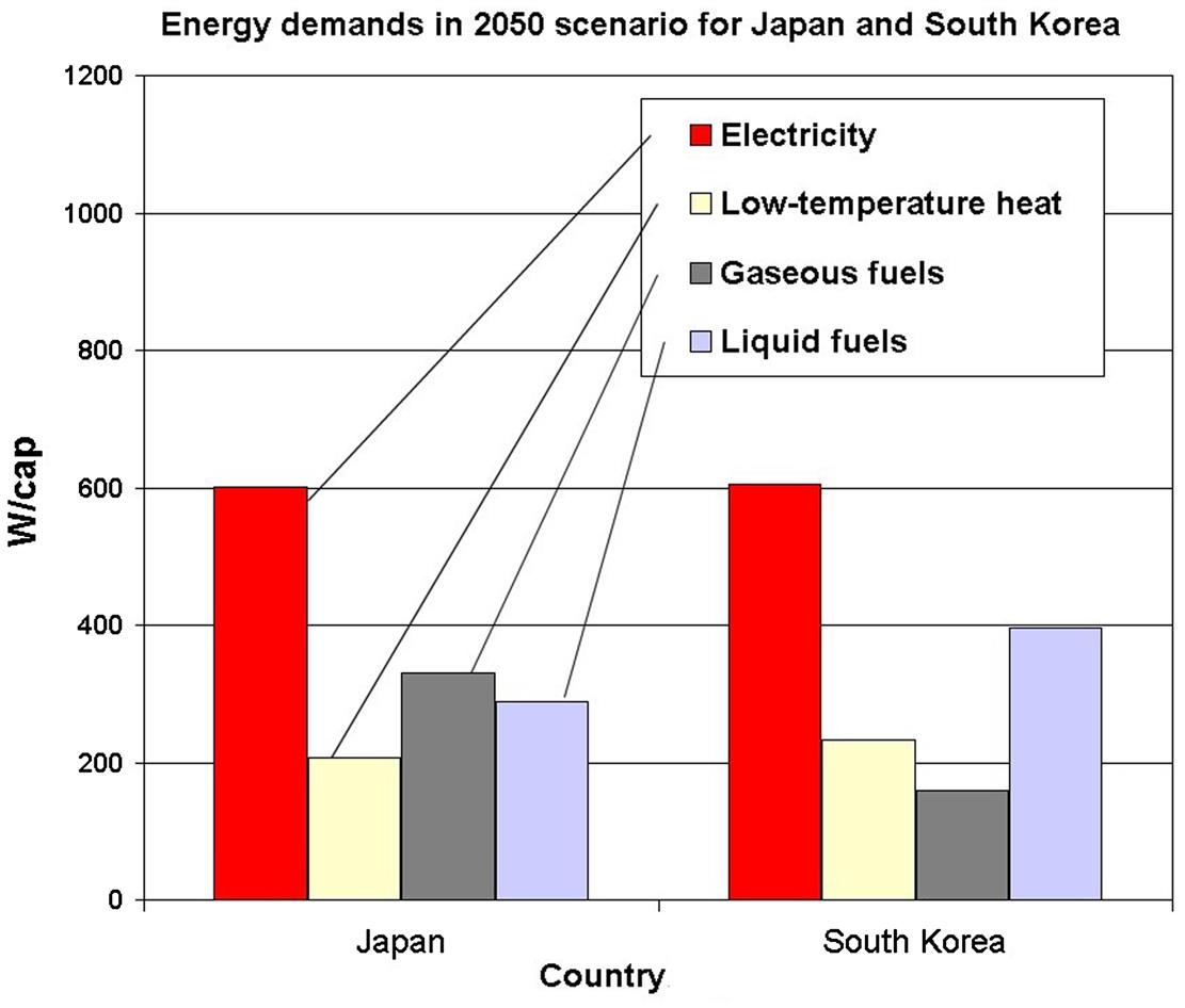
Figures 6.143 and 6.144 give an overview of the amounts of renewable energy actually used in the 2050 scenarios, and Figs. 6.145 and 6.146 show the outcome of the simulation calculations for Japan and South Korea. The heat provided by solar thermal collectors must be supplemented with electricity-driven heat pumps and by use of waste heat from the hydrogen production and stationary use processes. Because the temporal variation in wind power is extremely seasonal, particularly for Japan (Fig. 6.147), with a four month low during summer, there is a quite large requirement for storing hydrogen produced during the winter period for use during the summer wind lull (Fig. 6.148), despite using reservoir-based Japanese hydro as much as possible during the summer period (Sørensen, 2017). This is a reason for preferring fuel cell vehicles over battery-operated electric vehicles, as long-time storage of energy in batteries is far more expensive than hydrogen storage in underground cavities (aquifers or cavities washed out in salt dome intrusions, cf. Fig. 5.19). Because the seasonal peculiarities are similar for Japan and South Korea, little is gained by trading electricity or fuels between the two countries. In the North America scenario, the shorter-term variations in renewable energy production and the large differences in resource sizes made trade very attractive. For South Korea–Japan, the first can easily be accommodated in the operation of the large stores already needed for dealing with the large seasonal variations, and the resource sizes are similar. Only in April, where the for later use required maximum filling of the hydrogen stores is reached, would there be a modest export opportunity for Japan, contingent on establishing undersea transmission cables to South Korea. Still, adding transmission facilities will in any case augment supply security, as evidenced by the lack of adequate transmission options even within Japan at the time of the Fukushima nuclear power plant accident in 2011.

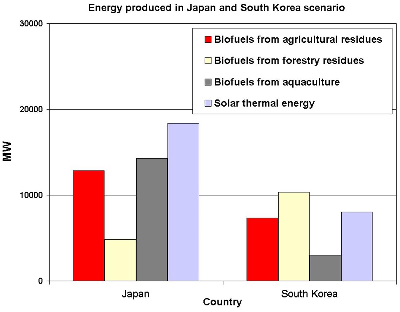
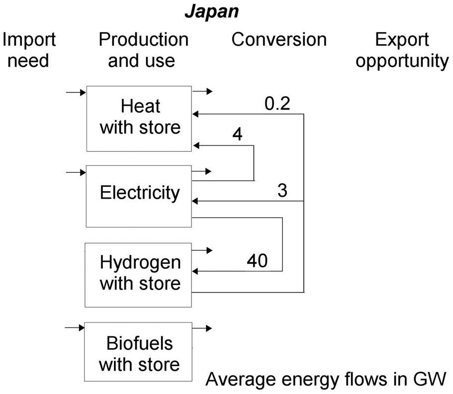
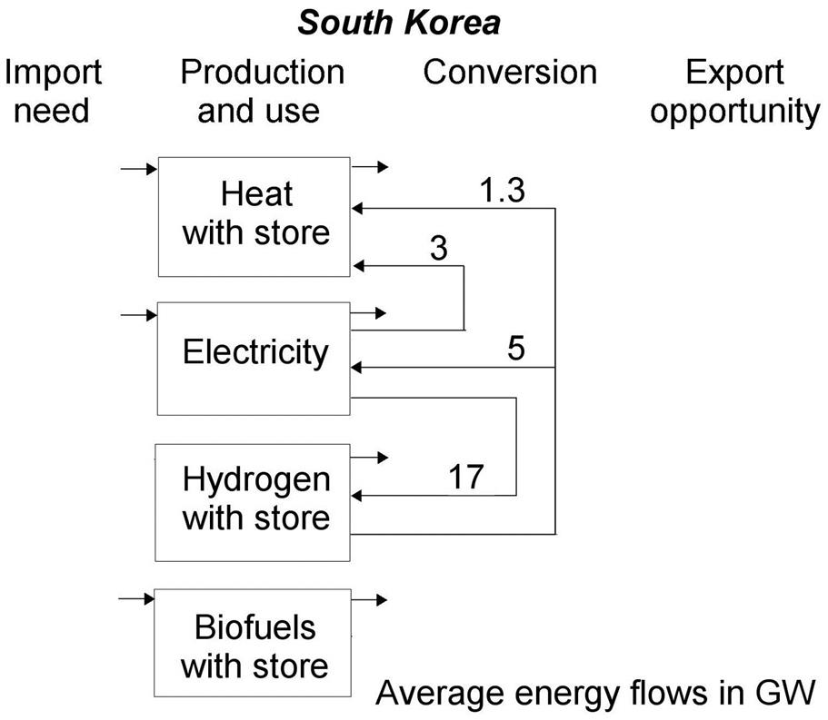


6.6.6 China
China is rich in renewable energy resources, as evident from Figs. 6.137 to 6.140. Solar radiation is very seasonal except for the most southern part of the country. Wind power is large in the western high country, in a belt from Mongolia and southward to the sea, and along the entire coast. Very spectacular are the offshore wind resources (Fig. 6.141), where the shallow waters toward the China Sea offer much larger areas of offshore wind parks at reasonable foundation depths than the steeper ocean floor descent found in section 6.6.5 near the southeastern shores of Japan. Run-off, shown in Fig. 6.139, is a proxy for hydro power, but in the Chinese case, the high values in the western plains (associated with precipitation from wet air blown across the Himalayas to colder areas) do not benefit hydro in those same areas, because there is no lower outlet to reflect the full height difference to sea level. However, some of the runoff is collected by rivers like the Yangtse, giving rise to a multitude of existing and planned Chinese hydro installations further downstream, particularly in Yunnan and Sichuan. Regarding biomass production (Fig. 6.140), the western high plains are very low, while the eastern part of China except for an area near Mongolia is quite fertile. Irrigation can increase the productivity in both the western and eastern parts of the country, and it might be possible to use some of the surplus run-off in the western region without disturbing groundwater flows. However, care should be taken only to create artificial irrigation in a way that does not diminish the feeding of water into the rivers used for hydro downstream. The pattern of renewable energy distribution over the Chinese land area is poorly correlated with the population distribution, which is highest in some of the eastern provinces (cf. Figs. 6.1 and 6.2). Therefore, electricity transmission and biofuel transport will play an important role in the construction of energy scenarios. For this reason, the country is, in the scenarios presented here, divided into four regions, not with regard to administrative divisions but just to better illustrate the energy planning and transfer requirements. The four regions are defined in Fig. 6.149, and their respective populations assumed for the 2050 scenario are given. A precursor scenario for China without considering regional differences and transfers was modeled in Sørensen (2015).
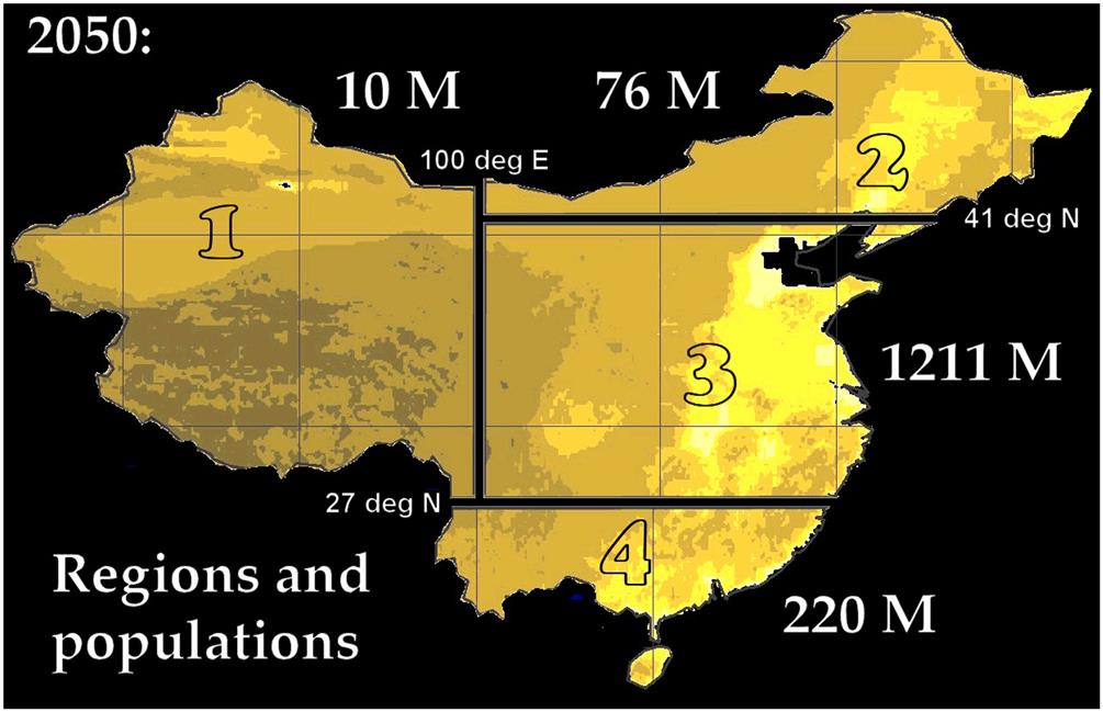
The overall Chinese energy demands in the four regions considered are presented in Fig. 6.150 for the scenario year 2050. As expected, the space heating variations make the low-temperature heat demand varies between regions, while the other energy forms are demanded similarly, per capita. The time-distribution of heat demands is shown in Fig. 6.151, including process heat used for hygiene and industrial processes below 100°C. The sparsely populated Region 1 has a transportation need similar to the other regions, because although the smaller number of industrial enterprises reduces need for transport of goods, the transport distances for all kinds of mobility are larger. For electricity, the time-distribution of European demands are used, due to the absence of guidance by data for current use in China.

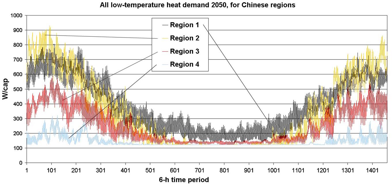
Figures 6.152 and 6.153 shows the renewable energy that can be produced in each of the Chinese regions, using conditions similar to those of the scenarios described above (wind turbine swept area 0.075% of the land surface plus 0.15% of offshore areas with water depth under 50 m, 1 m2/cap. of rooftop PV plus solar farms on 2.4% of marginal land, 40% of agricultural residues used for fuel production, 45% of forestry residues, and 50% of aquacultural biomass). Only the southwestern regions have offshore wind power, but Regions 1 and 2 have large onshore wind surpluses, and Region 1 could further produce large amounts of power from solar photovoltaic farms. As Fig. 6.153 shows, forestry residues are fairly modest, but agricultural residues are abundant in the three regions with extensive farming, needed of course for the large populations. Figure 6.154 shows the time-variations over a year of the surplus wind and solar power in Region 1, with a seasonality induced by the solar part, as the fluctuations in wind power is on a smaller scale (up to a week or two), with no overall seasonality, as also seen in Fig. 6.155 for the wind production in Region 3, onshore or offshore.
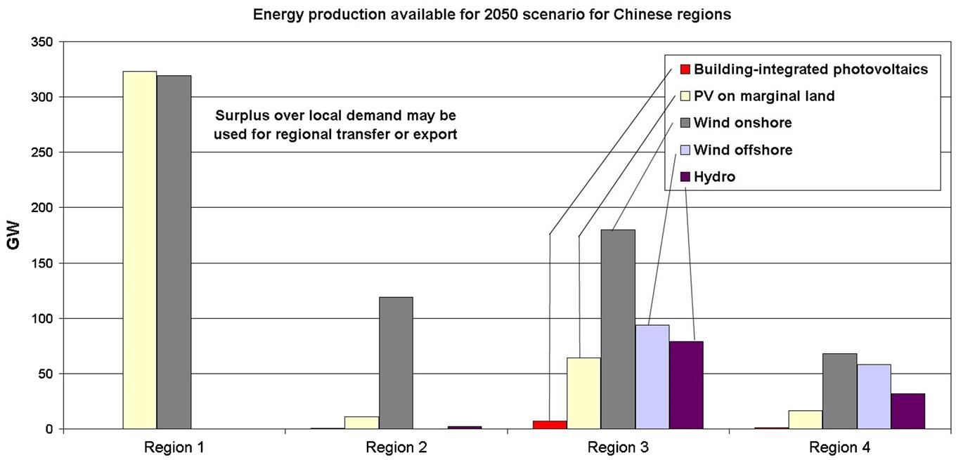
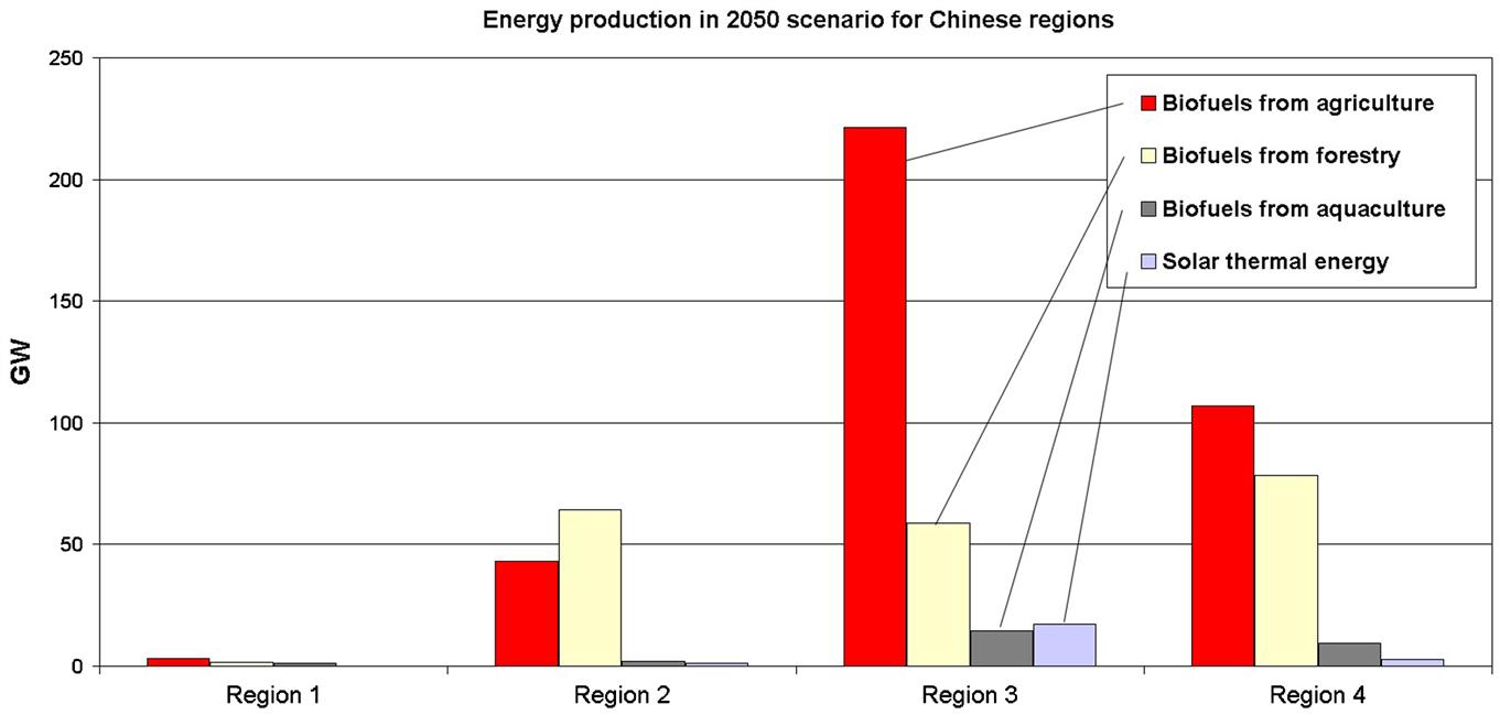
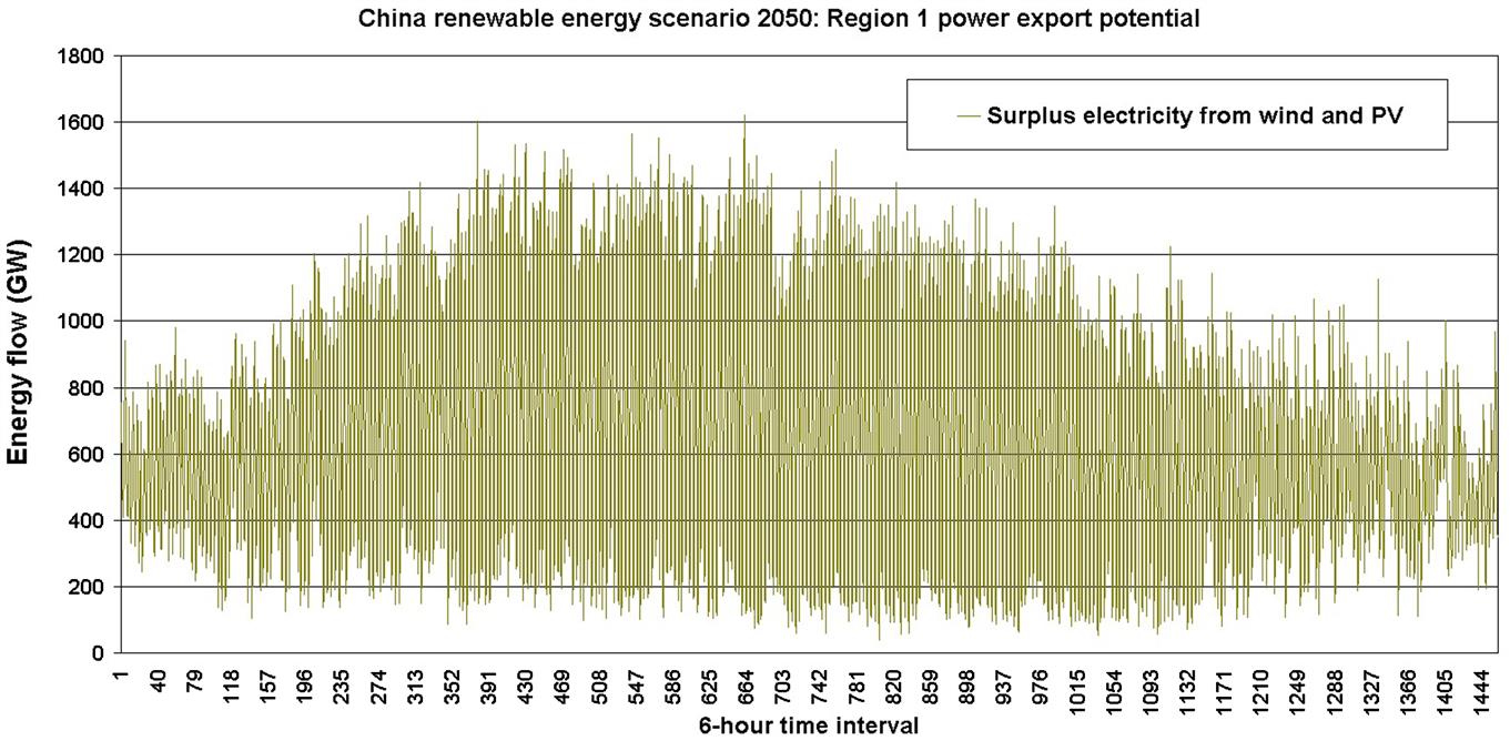

Matching demand and supply requires transfer of energy between the regions, and due to the short-term variations in wind and solar power (that is not sufficiently smoothed by combining output from different regions), there is a need for storage of electricity. As mentioned earlier, the cheapest way of accomplishing this is by underground hydrogen caverns. Figure 6.156 gives the variations in the degree of filling of these reservoirs in the largest consumption Region, number 3, derived from the overall simulation of the scenarios for each region. The storage capacity needed is relatively small compared to that of the Japan and South Korea scenarios, where large seasonal variations in wind power production had to be dealt with by energy storage. The introduction of hydrogen makes it reasonable to cover some of the transportation needs by hydrogen-fueled vehicles, in addition to using hydrogen for regeneration of electricity. All the hydrogen in the scenarios is in the first place produced by electrolysis. This also solves the problem of making surplus wind and solar power production useful, which in the absence of energy stores could be as difficult as covering the deficits.

Figures 6.157–6.160 summarize the Chinese regional scenarios. Only Region 3 has a need for importing energy from the three other regions, but this need is substantial and is present for all the energy forma. However, the imports need only be of electricity and biofuels, as heat can be derived from waste heat generated at each conversion (e.g. to and from hydrogen) or from electricity-driven heat pumps, and hydrogen is generated from the imported electricity. It is seen that surplus electricity from Regions 1, 2, and 4 is more than sufficient to cover the import needs for power, heat, and gaseous fuel in Region 3, while the Region 3 import need for biofuels just matches the surpluses from Regions 2 and 4. Should more be required, the share of hydrogen-fueled (fuel cell or hybrid) vehicles can be increased. In conclusion, China is endowed with sufficient renewable energy to allow the establishment of a stable and unstressed supply system, covering a demand as high as that of the most developed nations, say in Europe.
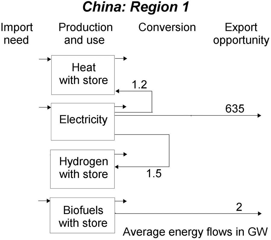
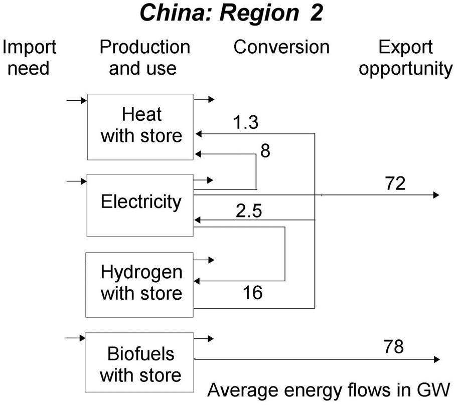
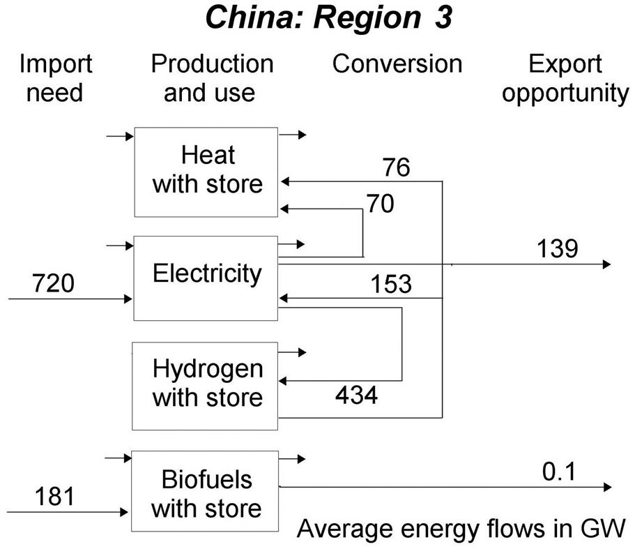
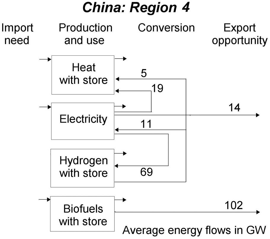
6.7 Global energy scenarios
The global scenarios presented in this section are from an early calculation (Sørensen & Meibom, 1998, 2000), using a much simpler model than those used in the regional scenarios above. Geographical resource data were available only as monthly means, and simplistic models had to be used for providing them with realistic short-term behavior (explained in the references; for wind also in the early part of section 6.3.2). The results thus only give a taste of the development of scenario techniques and yet results that in many ways resemble the more detailed calculations.
The global energy demand scenario for the year 2050 described in section 6.3 is used together with the simplified resource estimates to produce the results illustrated in the following. The supply–demand matching first uses only the renewable energy that is estimated to be available locally; subsequently, if necessary, more centralized production, such as offshore wind farms or photovoltaic farms on marginal land, are used. The study was probably the first to accept energy in food as part of the renewable energy concept. The reason is of course that some renewable energy sources have a double role, in both energy and nutrition, a possibility not applicable to fossil fuels.
The vegetable part of food production is shown in Fig. 6.161, which contains comparisons of local supply and demand, with Fig. 6.161a showing the amount of surplus for the geographical grid cells where supply exceeds demand, and Fig. 6.161b the amount of deficit for the local cells where demand exceeds supply. Regional sums are given in Table 6.11. It follows that, on average, year-2050 worldwide supply exceeds demand by 35%. This gives room for variations in crop harvests and thus variations in food production from year to year, as well as for differences in eating habits.
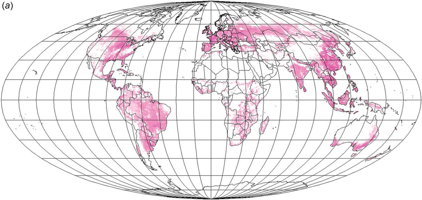

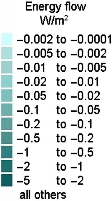

Table 6.11
Balance of potential regional food supply and demand in 2050 scenario.
| Region (cf. Table 6.5): | 1 | 2 | 3 | 4 | 5 | 6 | Total | Unit |
| Vegetable food | 108 | 113 | 91 | 192 | 40 | −140 | 402 | GW |
| Animal food | 43 | 31 | 16 | 91 | −63 | −27 | 91 | GW |
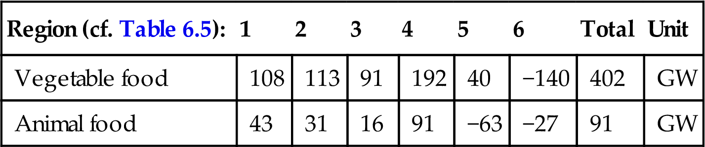
Like today, in year 2050 there is surplus vegetable food production in the Americas and Western Europe (Regions 1, 2, and 4, cf. Table 6.5) and by the year 2050 also in region 3 (including Russia), owing to proposed substantial improvements in agricultural practices assumed for this region. Region 5 (including China and India) will be barely self-sufficient by the year 2050, whereas Africa (Region 6) will have a deficit that must be covered by imports. In the scenario, Africa is the only region that by 2050 is in a development situation, where it may offer labor at lower expense than the other regions, and, thus, there will be the possibility of paying for food imports by industrial revenues, provided that an education policy is pursued that will give the workforce the necessary skills. In addition to interregional exchange, upon closer inspection, Fig. 6.161 allows a deduction of the requirements for transport of vegetable food within regions, e.g., from farming areas to cities.
The scenario assumptions for interregional trade in food are summarized in Fig. 6.172, where the regional exports have been selected from the surpluses available.
For animal-based food from either rangeland or fodder-fed animals, the surpluses and deficits are shown in Fig. 6.162. In Regions 1–4, the picture is similar to that for vegetable foods, with surpluses, but in Regions 5 and 6 there are deficits. This is due to the increase in the meat and milk fractions of diets assumed for Asia (Table 6.5), but the amounts are easily covered by imports from other regions, as indicated in Figs. 6.169 and 6.170. Overall, the animal food supply exceeds demand by 27%, which again is considered adequate in view of additional losses. Variations between years are smaller than for primary crops (because of the storage functions performed by livestock), but a reserve is required due to epidemics of animal diseases.

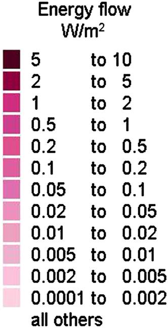
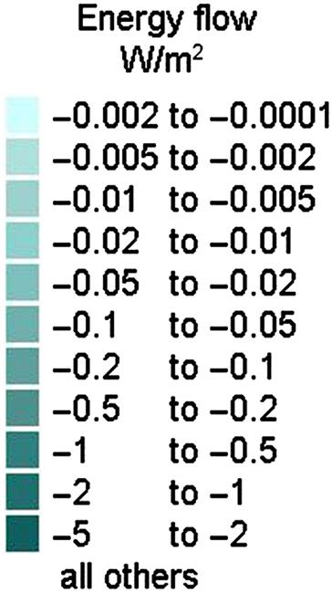
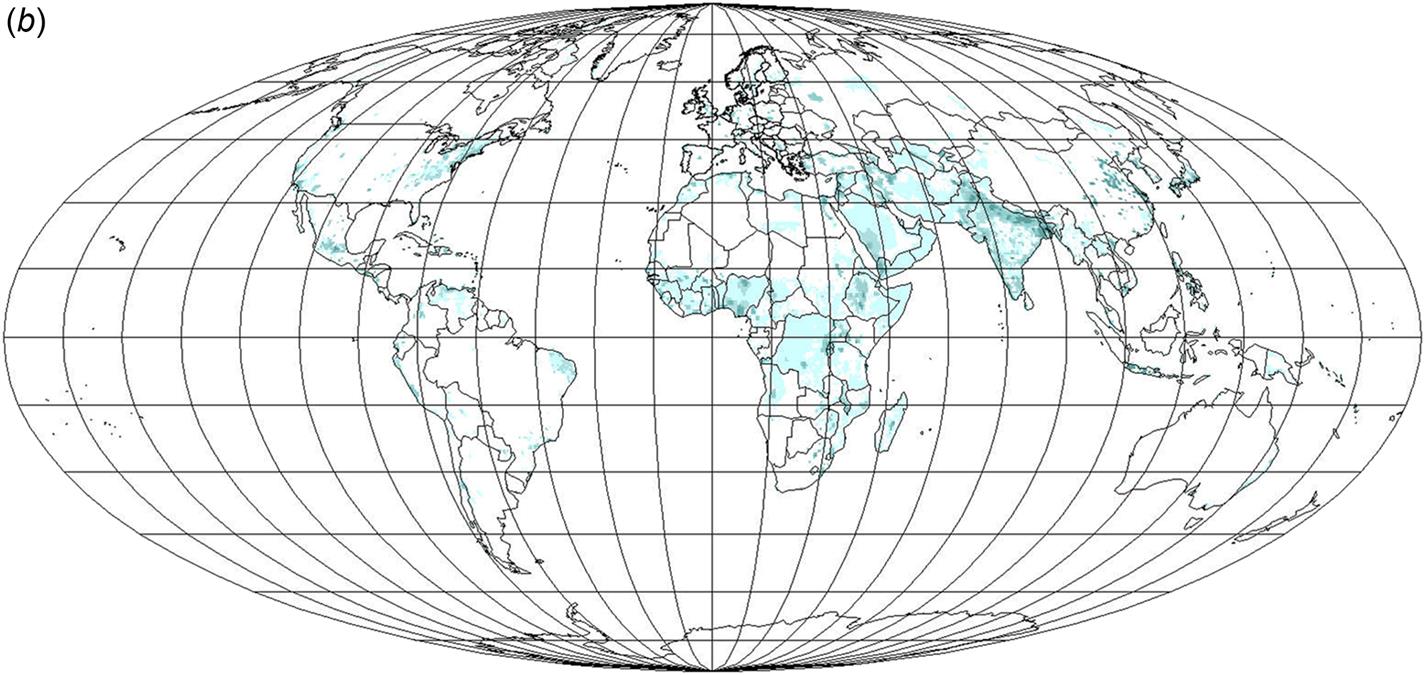
The regional energy sources employed to satisfy energy demands beyond food energy are listed in Table 6.12. For hydropower, existing plants and those already under construction are kept, but no additional plants are allowed to be built, in consideration of their environmental impacts. Untapped hydro resources are primarily in South America (cf. Fig. 3.49).
Table 6.12
Assumed energy supply (after storage conversion cycles and transmission but before interregional imports/exports) in the 2050 scenario, and corresponding supply–demand balances.
| Region (cf. Table 6.5) | 1 | 2 | 3 | 4 | 5 | 6 | Total | Unit |
| Total food balance (as in Table 6.10) | 151 | 144 | 107 | 283 | −23 | −167 | 493 | GW |
| Total biofuels used | 250 | 190 | 300 | 640 | 327 | 192 | 1899 | GW |
| Of which decentralized biofuels | 250 | 166 | 236 | 640 | 295 | 192 | 1779 | GW |
| Balance: total biofuels minus use for transportation | 136 | 158 | 146 | 277 | 392 | 61 | 1170 | GW |
| Hydropower | 80 | 70 | 50 | 120 | 110 | 10 | 440 | GW |
| Decentralized solar power | 27 | 50 | 67 | 109 | 189 | 23 | 465 | GW |
| Centralized solar power | 40 | 20 | 114 | 19 | 400 | 100 | 693 | GW |
| Decentralized wind power | 20 | 37 | 80 | 100 | 100 | 10 | 347 | GW |
| Onshore wind parks | 12 | 10 | 20 | 38 | 46 | 0 | 126 | GW |
| Offshore wind power | 0 | 40 | 0 | 0 | 13 | 0 | 53 | GW |
| Balance: other energy, annual average | 100 | −63 | 139 | 288 | −660 | 217 | 22 | GW |
| Balance: other energy, Jan. | 74 | −120 | 169 | 306 | −890 | 214 | −250 | GW |
| Balance: other energy, Apr. | 87 | −51 | 72 | 243 | −710 | 200 | −160 | GW |
| Balance: other energy, July | 129 | −17 | 180 | 352 | −410 | 233 | 461 | GW |
| Balance: other energy, Oct. | 110 | −64 | 129 | 252 | −610 | 220 | 35 | GW |

The sources proposed to be exploited in Table 6.12 are shown in Table 6.13 as fractions of the potential resources that they constitute. For region 4, current rainforest areas are not exploited but are left as preservation areas.
Table 6.13
Fraction of potential resources used in the 2050 scenario.
| Region (cf. Table 6.5) | 1 | 2 | 3 | 4 | 5 | 6 | Total |
| Decentralized biofuels | 0.91 | 0.98 | 0.96 | 0.93 | 1.00 | 0.92 | 0.94 |
| Centralized biofuels | 0 | 0.12 | 0.64 | 0 | 0 | 0 | 0.21 |
| Hydropower | 0.88 | 0.82 | 0.95 | 0.48 | 0.90 | 0.67 | 0.71 |
| Decentralized solar power | 0.54 | 0.93 | 0.71 | 0.76 | 0.99 | 0.20 | 0.72 |
| Centralized solar power | 0.013 | 0.003 | 0.014 | 0.004 | 0.041 | 0.005 | 0.013 |
| Decentralized wind power | 0.56 | 0.85 | 0.45 | 0.75 | 1.00 | 0.21 | 0.64 |
| Onshore wind parks | 0.75 | 0.068 | 0.27 | 0.66 | 1.00 | 0 | 0.21 |
| Offshore wind power | 0 | 0.52 | 0 | 0 | 0.70 | 0 | 0.16 |

The resulting energy system is very robust because there are additional renewable resources to use if the assumptions behind the scenario should turn out not to be right. This modesty is of course necessary, owing to the variations between seasons and years of renewable energy production, neither of which are, or can be, modeled precisely. Table 6.12 indicates substantial variations in supply–demand balances between seasons. Stores will have to handle the mismatch, and a detailed simulation is needed to ensure that it works, as was done for the regional scenarios of sections 6.5 and 6.6.
The area-based distributions of supply–demand balancing corresponding to the totals given in Table 6.12 are given in Fig. 6.163 for transportation biofuels and in Figs. 6.164 for stationary use of high-quality renewable energy sources. Figures 6.165–6.171 show block diagrams of the regional and global flows through the energy system from source to end-use.
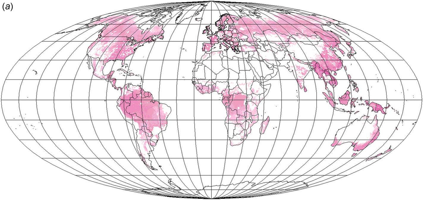
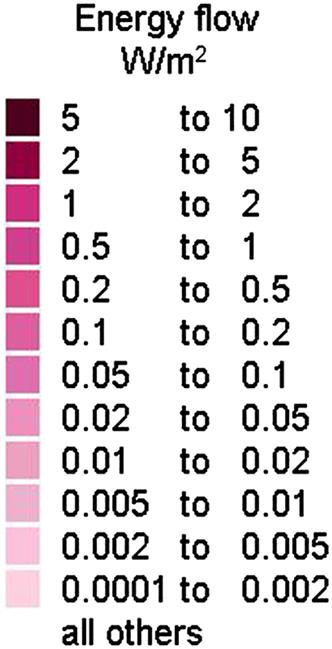


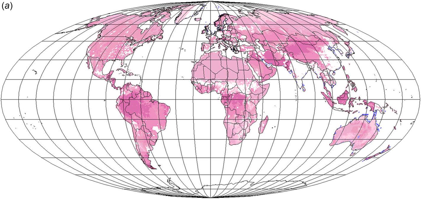
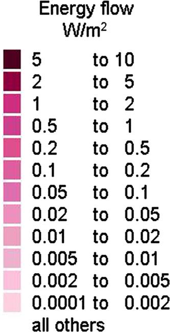

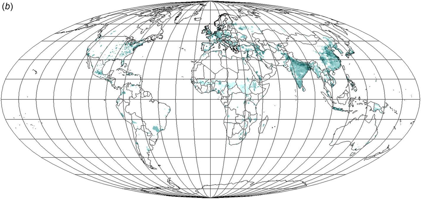

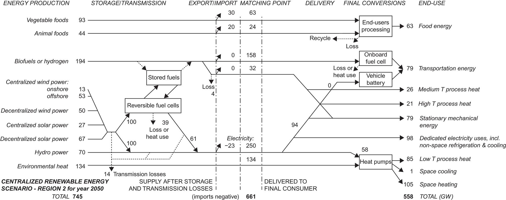


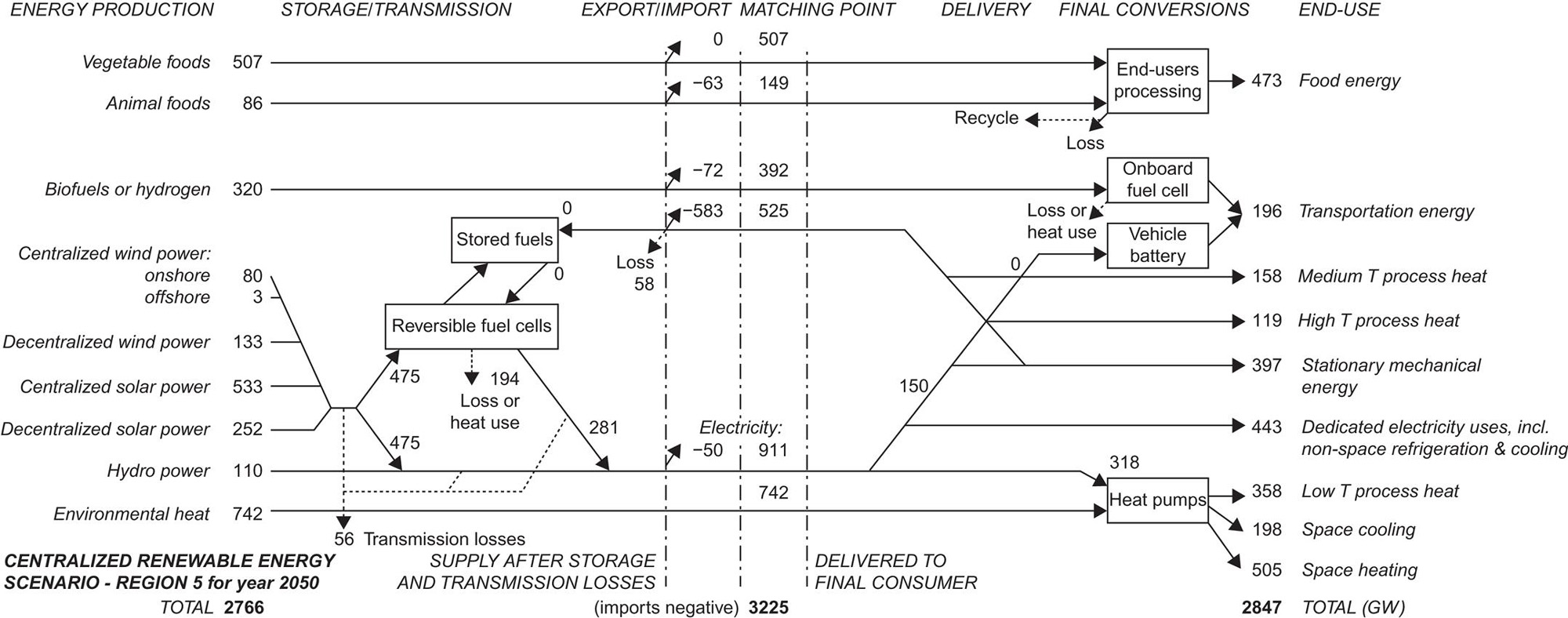

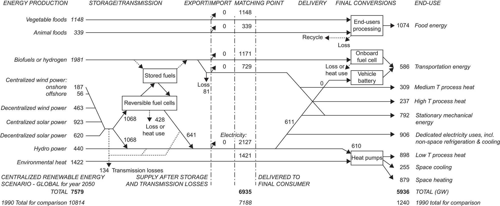

The main routes of import and export are depicted in Fig. 6.172. The amount of centralized energy used in the scenario is still modest compared to the potential listed in section 6.3, even when new large hydro installations or rainforest conversion are renounced. The PV and wind energy export options arising for desert land give such areas new opportunities for development and, in some cases, make up for current oil-export revenues lost. Also the large biofuel exports considered for South America give credibility to the assumed substantial economic development of this continent.
While it is not surprising that the most densely populated regions should have difficulty being self-sufficient in energy provision from renewable energy (Fig. 6.172), just as they usually are with the energy sources presently used, it is a little surprising to see how large a surplus of energy is offered for purchase by the regions with surplus renewable energy sources. This has implications for economic development (to be discussed in Chapter 7). The magnitude of these surpluses is illustrated in Table 6.13, which gives the percentages of estimated available resources actually used in the scenario.
This global scenario was made some time ago, and it is certainly not the only one possible. For example, the need in China for a large biofuel import can be avoided if transportation is based on electric or fuel cell vehicles instead of on internal combustion engines. This is precisely what the new Chinese scenario discussed in section 6.6 proposes to do. China gains independence from import of strategic energy commodities, but the new transportation modes presently looks considerably more expensive than biofuels, although this may not continue to be so. The Chinese scenario in section 6.6 also differs from the Chinese part of the global scenario by using more wind power, prompted by an improved technique for estimating particularly offshore potentials.