
where U may depend on wind speed in analogy to (4.118). The collector gain is now given by ![]() where the first term is proportional to A, while the two last terms are proportional to Aa. Assuming now a fluid flow
where the first term is proportional to A, while the two last terms are proportional to Aa. Assuming now a fluid flow ![]() through the absorber, the expression for determination of the amount of energy extracted becomes [cf. (4.128)]
through the absorber, the expression for determination of the amount of energy extracted becomes [cf. (4.128)]
(4.137)
where AaC′ is the heat capacity of the absorber and the relation between ![]() and Tc,out may be of the form (4.129) or (4.37). Inserting (4.114), with use of (4.134), (4.135), and (4.136), into (4.137), it is apparent that the main additional parameters specifying the focusing system are the area concentration ratio,
and Tc,out may be of the form (4.129) or (4.37). Inserting (4.114), with use of (4.134), (4.135), and (4.136), into (4.137), it is apparent that the main additional parameters specifying the focusing system are the area concentration ratio,
(4.138)
and the energy flux concentration ratio,
(4.139)
where tSW is given in (4.134) and Ai is the area of the actual image (which may be different from Aa). Knowledge of Ai is important for determining the proper size of the absorber, but it does not appear in the temperature equation (4.137), except indirectly through the calculation of the transmission function tSW.
For a stalled collector, ![]() and
and ![]() give the maximum absorber temperature Tc,max. If this temperature is high, and the wind speed is low, the convective heat loss (4.138) is negligible in comparison with (4.135), yielding
give the maximum absorber temperature Tc,max. If this temperature is high, and the wind speed is low, the convective heat loss (4.138) is negligible in comparison with (4.135), yielding
where D is the incident short-wavelength flux in the direction of the Sun [cf. (4.114)], assuming the device accepts only the flux from this direction and assuming perfect transmission to the absorber (tSW=1). With the same conditions, the best performance of an operating collector is obtained from (4.139), assuming a steady-state situation. The left-hand side of (4.139) is the amount of energy extracted from the collector per unit of time, Eextr:
(4.140)
and the efficiency corresponding to the idealized assumptions
(4.141)
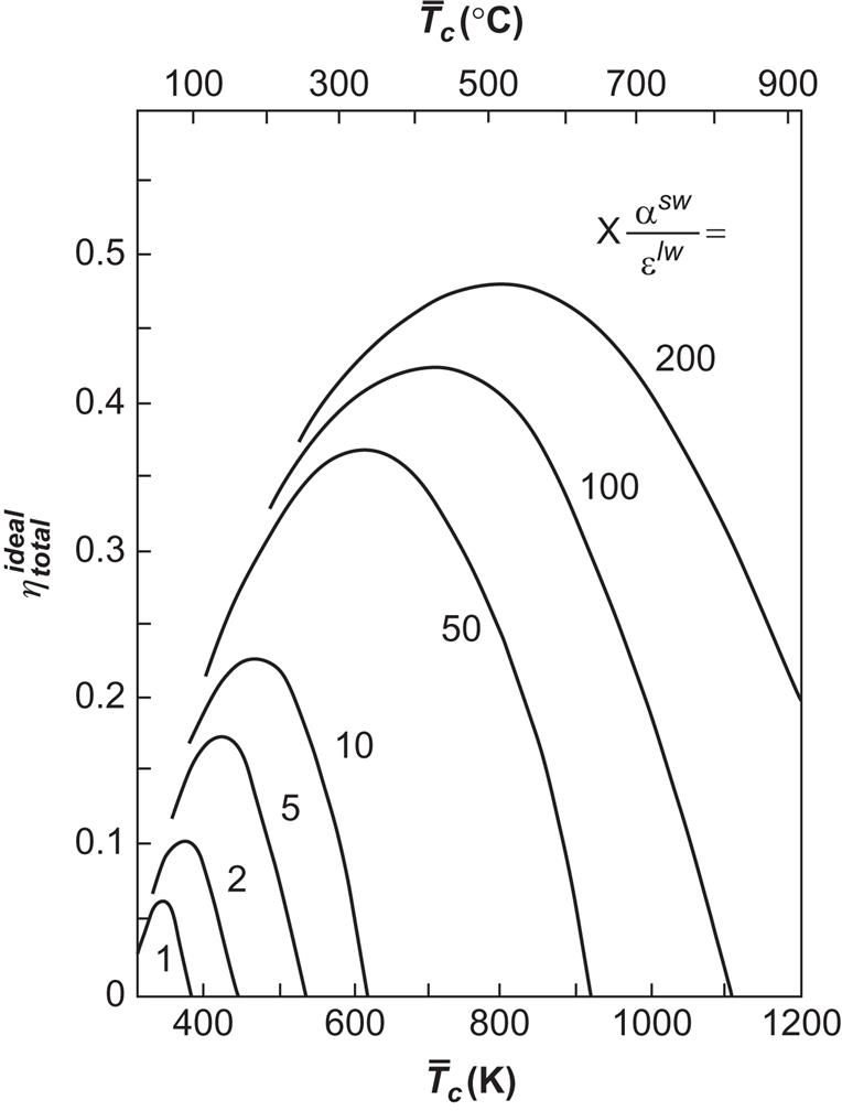
This relation is illustrated in Fig. 4.90, assuming D=800 W m−2, Te=300 K, and αSW=0.9, independent of absorber temperature. It is clear that the use of a selective absorber surface (large ratio αSW/εlw) allows a higher efficiency to be obtained at the same temperature and that the efficiency drops rapidly with decreasing light intensity D. If the total short-wavelength flux on the collector is substantially different from the direct component, the actual efficiency relative to the incident flux ![]() of (3.15),
of (3.15),
may be far less than the “ideal” efficiency (4.141).

4.4.4.2 Solar-thermal electricity generation
Instead of using photovoltaic or photo-electrochemical devices, one can convert solar radiation into electric energy in two steps: first, by converting radiation to heat, as described in section 4.4.3, or more likely by use of concentrating devices, as described above; and second, converting heat into electricity, using one of the methods described in sections 4.1.2 and 4.2.2. (Two-step conversion using chemical energy rather than heat as the intermediate energy form is also possible, for instance, by means of the photogalvanic conversion scheme briefly mentioned in section 4.5.2.) Examples of the layout of systems capable of performing solar heat to electric power conversion using thermodynamic cycles are given below, with discussion of efficiencies believed attainable.
4.4.4.3 Photo-thermoelectric converter design
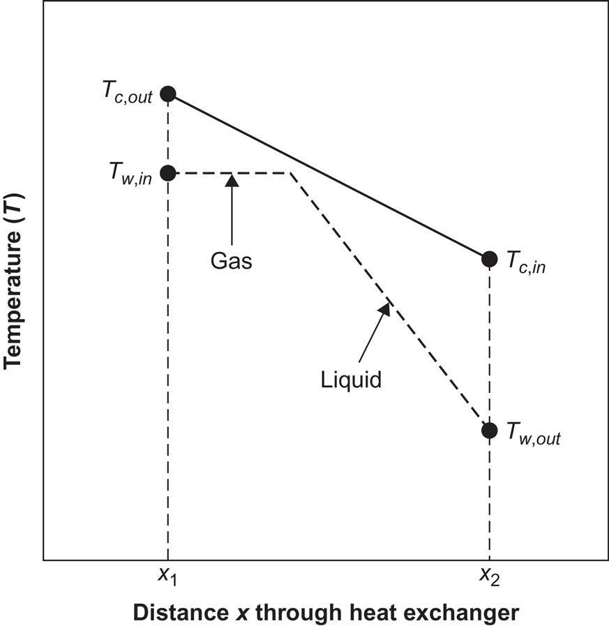
A two-step conversion device may be of the general form shown in Fig. 4.91. The solar collector may be the flat-plate type or it may perform a certain measure of concentration, requiring partial or full tracking of the Sun. The second step is performed by a thermodynamic engine cycle, for example, a Rankine cycle with expansion through a turbine, as indicated in the figure. Owing to the vaporization of the engine-cycle working fluid in the heat exchanger linking the two conversion steps, the heat exchange performance does not follow the simple description leading to (4.37). The temperature behavior in the heat exchanger is more like the type shown in Fig. 4.92. The fluid in the collector circuit experiences a uniform temperature decrease as a function of the distance traveled through the heat exchanger, from x1 to x2. The working fluid entering the heat exchanger at x2 is heated to the boiling point, after which further heat exchange is used to evaporate the working fluid (and perhaps superheat the gas), so that the temperature curve becomes nearly flat after a certain point.
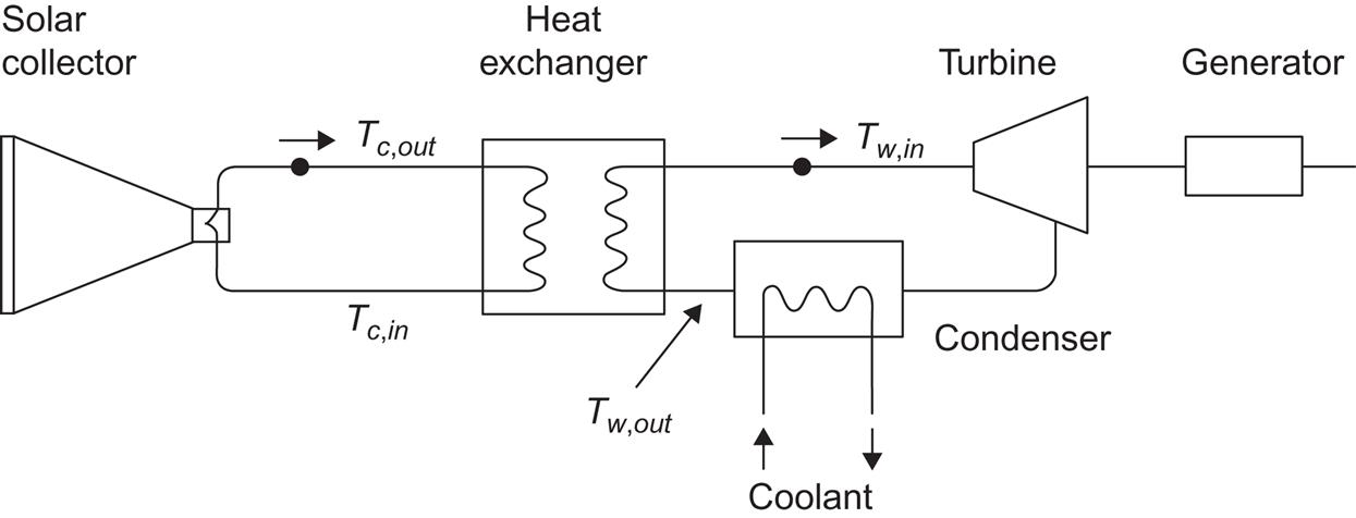
The thermodynamic engine cycle (the right-hand side of Fig. 4.91) can be described by the method outlined in sections 4.1.1 and 4.1.2, with the efficiency of heat to electricity conversion given by (4.19) [limited by the ideal Carnot process efficiency (4.4)],
where ![]() is the electric power output [cf. (4.14)] and
is the electric power output [cf. (4.14)] and
is the rate of heat transfer from the collector circuit to the working-fluid circuit in the heat exchanger. The right-hand side is given by (4.137) for a concentrating solar collector and by (4.128) and (4.124) for a flat-plate collector. The overall conversion efficiency is the product of the efficiency ηc of the collector system and ηw,
Determination of the four temperatures Tc,in, Tc,out, Tw,in, and Tw,out (cf. Fig. 4.91) requires an equation for collector performance, for heat transfer to the collector fluid, for heat transfer in the heat exchanger, and for processes involving the working fluid of the thermodynamic cycle. If collector performance is assumed to depend only on an average collector temperature, ![]() [e.g., given by (4.127)], and if Tw,in is considered to be roughly equal to
[e.g., given by (4.127)], and if Tw,in is considered to be roughly equal to ![]() (Fig. 4.92 indicates that this may be a fair first-order approximation), then the upper limit for ηw is approximately
(Fig. 4.92 indicates that this may be a fair first-order approximation), then the upper limit for ηw is approximately
Taking Tw,out as 300 K (determined by the coolant flow through the condenser in Fig. 4.91), and replacing ηc by the idealized value (4.141), the overall efficiency may be estimated as shown in Fig. 4.93, as a function of ![]() The assumptions for
The assumptions for ![]() are as in Fig. 4.90: no convective losses (this may be important for flat-plate collectors or collectors with a modest concentration factor) and an incident radiation flux of 800 W m−2 reaching the absorber (for strongly focusing collectors this also has to be direct radiation). This is multiplied by
are as in Fig. 4.90: no convective losses (this may be important for flat-plate collectors or collectors with a modest concentration factor) and an incident radiation flux of 800 W m−2 reaching the absorber (for strongly focusing collectors this also has to be direct radiation). This is multiplied by ![]() (the Carnot limit) to yield
(the Carnot limit) to yield ![]() depicted in Fig. 4.93, with the further assumptions regarding the temperature averaging and temperature drops in the heat exchanger that allow the introduction of
depicted in Fig. 4.93, with the further assumptions regarding the temperature averaging and temperature drops in the heat exchanger that allow the introduction of ![]() as the principal variable both in
as the principal variable both in ![]() and in
and in ![]()
In realistic cases, the radiation reaching the absorber of a focusing collector is perhaps half of the total incident flux ![]() and
and ![]() is maybe 60% of the Carnot value, i.e.,
is maybe 60% of the Carnot value, i.e.,
This estimate may also be valid for small concentration values (or, rather, small values of the parameter Xαsw/εlw characterizing the curves in Figs. 4.93 and 4.90), since the increased fraction of ![]() being absorbed is compensated for by high convective heat losses. Thus, the values of
being absorbed is compensated for by high convective heat losses. Thus, the values of ![]() between 6% and 48%, obtained in Fig. 4.93 for suitable choices of
between 6% and 48%, obtained in Fig. 4.93 for suitable choices of ![]() (which can be adjusted by altering the fluid flow rate
(which can be adjusted by altering the fluid flow rate ![]() ), may correspond to realistic efficiencies of 2–15%, for values of Xαsw/εlw increasing from 1 to 200.
), may correspond to realistic efficiencies of 2–15%, for values of Xαsw/εlw increasing from 1 to 200.
The shape of the curves in Fig. 4.93 is brought about by the increase in ![]() as a function of
as a function of ![]() counteracted by the accelerated decrease in
counteracted by the accelerated decrease in ![]() as a function of
as a function of ![]() which is seen in Fig. 4.90.
which is seen in Fig. 4.90.
Photo-thermoelectric conversion systems based on flat-plate collectors have been discussed, for example, by Athey (1976); systems based on solar collectors of the type shown in Fig. 4.88d have been considered by Meinel and Meinel (1972). They estimate that a high temperature on the absorber can be obtained by use of selective surfaces, evacuated tubes (e.g., made of glass with a reflecting inner surface except for the window shown in Fig. 4.88d), and a crude Fresnel lens (see Fig. 4.89) concentrating the incoming radiation on the tube window. Molten sodium is suggested as the collector fluid. Finally, fully tracking systems based on the concept shown on the right-hand side of Fig. 4.87 (“power towers”) have been proposed by Teplyakov and Aparisi (1976) and by Hildebrandt and Vant-Hull (1977). This concept is used in several installations, the best known of which is the Odeillo plant in southern France (Trombe and Vinh, 1973), which originally aimed at achieving temperatures for metalwork that exceeded those possible at fossil-fuel furnaces.
4.4.4.4 Optical subsystem and concentrators
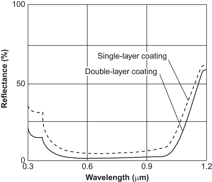
As indicated by the devices shown in Figs. 4.57 and 4.60, optical manipulation of incoming solar radiation is used in non-concentrating solar cells. These measures serve the purpose of reducing the reflection on the surface to below a few percent, over the wavelength interval of interest for direct and scattered solar radiation, as seen from Fig. 4.94. Their collection efficiency is far better than that shown on Fig. 4.54, exceeding 90% for wavelengths between 0.4 and 1.05 μm, and exceeding 95% in the interval 0.65–1.03 μm.
For large-factor concentration of light onto a photovoltaic cell much smaller than the aperture of the concentrator, the principles mentioned for thermal systems (discussion of Fig. 4.90) apply unchanged. Most of these concentrators are designed to focus the light onto a very small area, and thus tracking the Sun (in two directions) is essential, with the implications that scattered radiation largely cannot be used and that the expense and maintenance of non-stationary components have to be accepted.
One may think that abandoning very high concentration would allow the construction of concentrators capable of accepting light from most directions (including scattered light). However, this is not easy. Devices that accept all angles have a concentration factor of unity (no concentration), and even if the acceptance angular interval is diminished to, say, 0°–60°, which would be suitable because light from directions with a larger angle is reduced by the incident cosine factor, only a very small concentration can be obtained (examples like the design by Trombe are discussed in Meinel and Meinel, 1976).
The difficulty may be illustrated by a simple two-dimensional ray-tracing model of an (arbitrarily shaped) absorber, i.e., the PV cell, sitting inside an arbitrarily shaped concentrator (trough) with reflecting inner sides, and possibly with a cover glass at the top that could accommodate some texturing or lens structure. The one component that unfortunately is not available is a semitransparent cover that fully transmits solar radiation from one side and fully reflects the same wavelengths of radiation hitting the other side. With such a cover, nearly 100% of the radiation coming from any direction could reach the absorber, the only exception being rays being cyclically reflected into paths never reaching the absorber.
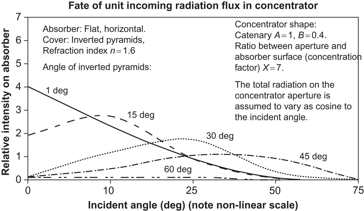
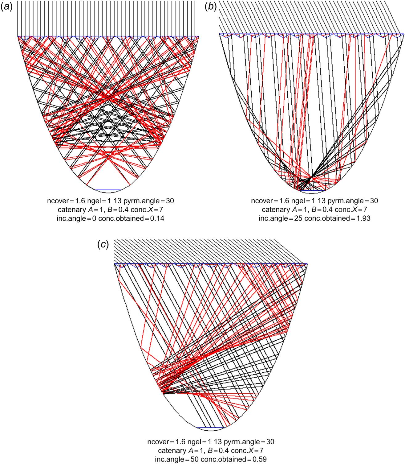
Figure 4.96 shows some ray-tracing experiments for a catenary-shaped concentrator holding a flat absorber at the bottom, with a concentration factor X=7 (ratio of absorber and aperture areas, here lines). The cover has an inverted pyramid shape. This is routinely used for flat-plate devices (see Fig. 4.57), with the purpose of extending the path of the light rays inside the semiconductor material so that absorption is more likely. For the concentrator, the purpose is only to make it more likely that some of the rays reach the absorber, by changing their direction from one that would not have led to impact onto the absorber. However, at the same time, some rays that otherwise would have reached the absorber may now become diverted. Thus, not all incident angles benefit from the concentrator, and it has to be decided whether the desired acceptance interval is broad (say, 0°–60°) or can be narrowed, e.g., to 0°–30°. As illustrated, the concentration of rays toward the center absorber is paid for by up to half of the incident rays’ being reflected upward after suffering total reflection on the lower inside of the cover glass.
The result of varying some of the parameters is shown in Fig. 4.95. An inverted pyramid angle of 0° corresponds to a flat-plate glass cover, and the figure shows that in this situation the concentration is limited to incident angles below 20°, going from a factor of four to unity. With increasing pyramid angle, the maximum concentration is moved toward higher incident angles, but its absolute value declines. The average concentration factor over the ranges of incident angles occurring in practice for a fixed collector is not even above unity, meaning that a PV cell without the concentrating device would have performed better.
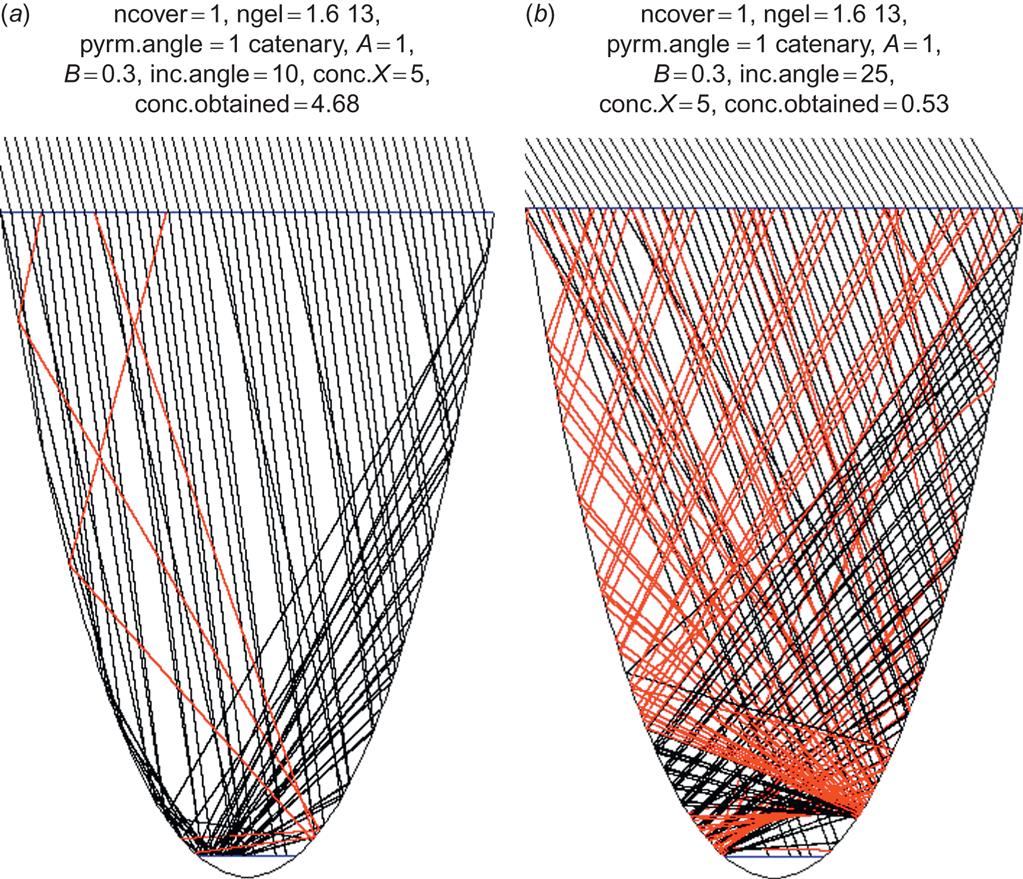
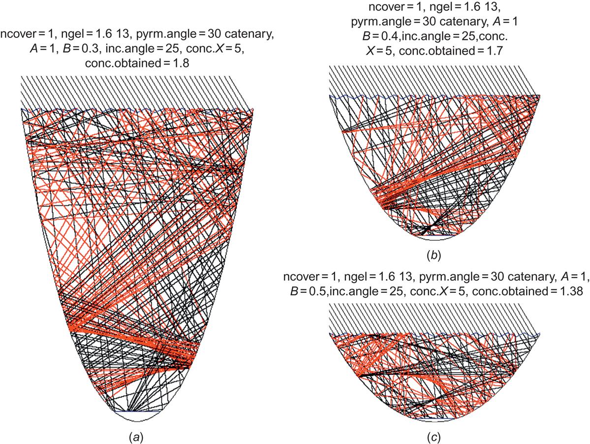
Another idea is to direct the cover pyramids upward, but to avoid “stretching out” the rays again at the lower glass boundary by having the entire trough filled with the refractive substance (which might be a gel or plastic material, textured at the upper surface). This is illustrated in Figs. 4.97a–c for an X=5 concentrator. For a deep catenary-shaped collector, all rays up to 10° may be led to the absorber, but in this case (Figs 4.97a and 4.98), incident angles above 25° are not accepted. To get reasonable acceptance, pyramid angles around 30° would again have to be chosen, and Figs. 4.97a–c show that the concentration penalty in trying to extend the acceptance interval to angles above 35° (by decreasing the depth of the concentrator, see Fig. 4.99) is severe. The best choice is still the deep catenary shape, with maximum concentration between 2 and 3 and average concentration over the interesting interval of incident angles (say, to 60°) no more than about 1.5. This is better than the inverted pyramid structure in Fig. 4.96, but it is still doubtful whether the expense of the concentrator is warranted. The collector efficiency, as measured relative to total aperture area, is the ratio of absorber intensity and X, i.e., considerably less than the cell efficiency.

Generation 24 h a day at constant radiation intensity could be achieved by placing the photovoltaic device perpendicular to the direction of the Sun at the top of the Earth’s atmosphere. Use of photovoltaic energy systems is, as mentioned, common on space vehicles and also on satellites in orbit around the Earth. It has been suggested that, if a large photovoltaic installation were placed in a geosynchronous orbit, the power generated might be transmitted to a fixed location on the surface of the Earth, after having been converted to microwave frequency (see, for example, Glaser, 1977).
4.4.5 Solar cooling and other applications
A variety of other applications of solar energy thermal conversion have been considered. Comfortable living conditions and food preservation require cooling in many places. As in the case of heating, the desired temperature difference from the ambient is usually only about 10–30°C. Passive systems like those depicted in Figs. 4.76 and 4.77 may supply adequate cooling in the climatic regions for which they were designed. Radiative cooling is very dependent on the clearness of the night sky (cf. section 3.1.4). It is only recently that materials have been identified that can provide more daytime cooling (by thermal emission) than warming from device heating. The idea is to reflect as much sunlight as possible by an integrated photonic reflector consisting of several layers of HfO2 and SiO2 with individually optimized thickness, and 97% reflection has been achieved (Raman et al., 2014).
In desert regions with a clear night sky, the difference between the winter ambient temperature and the effective temperature of the night sky has been used to freeze water. In Iran, the ambient winter temperature is typically a few degrees Celsius above the freezing point of water, but the temperature Te of the night sky is below 0°C. In previous centuries, ice (for use in the palaces of the rich) was produced from shallow ponds surrounded by walls to screen out daytime winter sunlight, and the ice produced during the night in such natural icemakers (“yakhchal,” see Bahadori, 1977) could be stored for months in very deep (say, 15 m) underground containers.
Many places characterized by hot days and cool nights have taken advantage of the heat capacity of thick walls or other structures to smooth out the diurnal temperature variations. If additional cooling is required, active solar cooling systems may be employed, and “cold storage” may be introduced to cover the cooling requirement independent of variations in solar radiation, in analogy to “hot storage” of solar heating systems.
A solar cooling system may consist of flat-plate collectors delivering the absorbed energy to a “hot storage,” which is then used to drive an absorption cooling cycle (Fig. 4.100), drawing heat from the “cool storage,” to which the load areas are connected (see, for example, Wilbur and Mancini, 1976). In principle, only one kind of storage is necessary, but, with both hot and cold storage, the system can simultaneously cover both heating needs (e.g., hot water) and cooling needs (e.g., air conditioning).
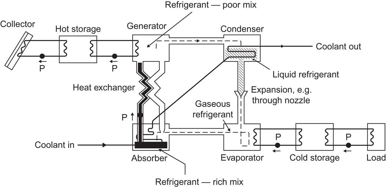
The absorption cooling cycle (Fig. 4.100) is achieved by means of an absorbent–refrigerant mix, such as LiBr–H2O or H2O–NH3. The lithium–bromide–water mix is more suitable for flat-plate solar collector systems, having a higher efficiency than the water–ammonia mix for the temperatures characteristic of flat-plate collectors. LiBr is hygroscopic, i.e., it can mix with water in any ratio. Solar heat is used in a “generator” to vaporize some water from the mix. The resulting vapor is led to a condenser unit, using a coolant flow, and is then expanded to regain a gaseous phase, whereby it draws heat from the area to be cooled, and subsequently is returned to an “absorber” unit. Here it becomes absorbed in the LiBr–H2O mix with the help of a coolant flow. The coolant inlet temperature would usually be the ambient one, and the same coolant passes through the absorber and the condenser. The coolant exit temperature would then be above ambient, and the coolant cycle could be made closed by exchanging the excess heat with the surroundings (e.g., in a “cooling tower”). The refrigerant-rich mix in the absorber is pumped back to the generator and is made up for by recycling refrigerant-poor mix from the generator to the absorber (e.g., entering through a spray system). In order not to waste solar heat or coolant flow, these two streams of absorbent–refrigerant mix are made to exchange heat in a heat exchanger. The usefulness of a given absorbent–refrigerant pair is determined by the temperature dependence of vaporization and absorption processes.
In dry climates, a very simple method of cooling is to spray water into an airstream (evaporative cooling). If the humidity of the air should remain unchanged, the air has first to be dried (spending energy) and then cooled by evaporating water into it, until the original humidity is again reached.
In principle, cooling by means of solar energy may also be achieved by first converting the solar radiation to electricity by one of the methods described in sections 4.4.1, 4.4.2, or 4.4.4 and then using the electricity to drive a thermodynamic cooling cycle, such as the Rankine cycle in Fig. 4.3.
The same applies if the desired energy form is mechanical work, as in the case of pumping water from a lower to a higher reservoir (e.g., for irrigation of agricultural land). In practice, however, the thermodynamic cycles discussed in section 4.1.2 are used directly to make a pump produce mechanical work on the basis of the heat obtained from a solar collector. Figure 4.101 shows two types of devices based on the Stirling cycle, using air or another gas as a working fluid (cf. Fig. 4.3). In the upper part of the figure, two ball valves ensure an oscillatory, pumping water motion, maintained by the tendency of the temperature gradient in the working fluid (air) to move air from the cold to the hot region. The lower part of the figure shows a “free piston Stirling engine,” in which the oscillatory behavior is brought about by the presence of two pistons of different mass, the heavy one being delayed by half an oscillatory period with respect to the lighter one. The actual water pumping is done by the “membrane movements” of a diaphragm, but if the power level is sufficient, the diaphragm may be replaced by a piston pump. For Stirling cycle operation, the working fluid is taken as a gas. This is an efficient cycle at higher temperatures (e.g., with use of a focusing solar collector), but if the heat provided by the (flat-plate) solar collector is less than about 100°C, a larger efficiency may be obtained by using a two-phase working fluid (corresponding to one of the Rankine cycles shown in Fig. 4.3). If focusing solar collectors are used, the diaphragm may be replaced by a more efficient piston pump.

Two Rankine-type solar pumps, based on a fluid-to-gas and gas-to-fluid cycle, are outlined in Fig. 4.102. The one shown in the upper part of the figure is based on a cyclic process. The addition of heat evaporates water in the container on the left, causing water to be pumped through the upper one-way valve. When the vapor reaches the bottom of the U-tube, all of it moves to the container on the right and condenses. New water is drawn from the bottom reservoir, and the pumping cycle starts all over again. This pump is intended for wells of shallow depth, below 10 m (Boldt, 1978).
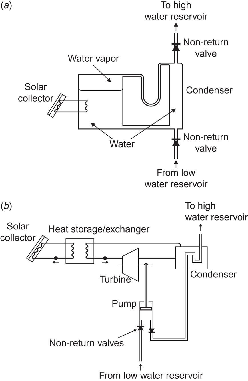
Figure 4.102b shows a pump operated by a conventional Rankine engine, expanding the working fluid to the gas phase and passing it through a turbine, and then condensing the gas using the pumped water as coolant, before returning the working fluid to the heat exchanger receiving solar absorbed heat. For all the pumps based on a single thermodynamic cycle, the maximum efficiency (which cannot be reached in a finite time) is given by (4.4) and the actual efficiency is given by an expression of the form (4.19).
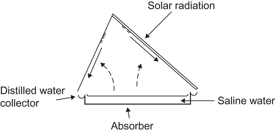
Distillation of saline water (e.g., seawater) or impure well water may be obtained by a solar still, a simple example of which is shown in Fig. 4.103. The side of the cover system facing the Sun is transparent, whereas the part sloping in the opposite direction is highly reflective and thus remains at ambient temperature. It therefore provides a cold surface for condensation of water evaporated from the saline water surface (kept at elevated temperature due to the solar collector part of the system). In more advanced systems, some of the heat released by condensation (about 2.3 × 10⁶ J kg−1, which is also the energy required for vaporization) is recovered and used to heat more saline water (Talbert et al., 1970).
4.5 Electrochemical energy conversion
Electrochemical energy conversion is the direct conversion of chemical energy, i.e., free energy of the form (4.8), into electrical power or vice versa. A device that converts chemical energy into electric energy is called a fuel cell (if the free energy-containing substance is stored within the device rather than flowing into the device, the term primary battery is sometimes used). A device that accomplishes the inverse conversion (e.g., electrolysis of water into hydrogen and oxygen) may be called a driven cell. The energy input for a driven cell need not be electricity, but could be solar radiation, for example, in which case the process would be photochemical rather than electrochemical. If the same device can be used for conversion in both directions, or if the free energy-containing substance is regenerated outside the cell (energy addition required) and recycled through the cell, it may be called a regenerative or reversible fuel cell and, if the free energy-containing substance is stored inside the device, a regenerative or secondary battery.
The basic ingredients of an electrochemical device are two electrodes (sometimes called anode and cathode) and an intermediate electrolyte layer capable of transferring positive ions from the negative to the positive electrode (or negative ions in the opposite direction), while a corresponding flow of electrons in an external circuit from the negative to the positive electrode provides the desired power. Use has been made of solid electrodes and fluid electrolytes (solutions), as well as fluid electrodes (e.g., in high-temperature batteries) and solid electrolytes (such as ion-conducting semiconductors). A more detailed treatise on fuel cells may be found in Sørensen (2012).
4.5.1 Fuel cells
The difference in electric potential, Δϕext, between the electrodes (cf. the schematic illustration in Fig. 4.104) corresponds to an energy difference eΔϕext for each electron. The total number of electrons that could traverse the external circuit may be expressed as the product of the number of moles of electrons, ne, and Avogadro’s constant NA, so the maximum amount of energy emerging as electrical work is
(4.142)
where ![]() (Faraday’s constant) is sometimes introduced. This energy must correspond to a loss (conversion) of free energy,
(Faraday’s constant) is sometimes introduced. This energy must correspond to a loss (conversion) of free energy,
(4.143)
which constitutes the total loss of free energy from the “fuel” for an ideal fuel cell. This expression may also be derived from (4.8), using (4.2) and ΔQ=TΔS, because the ideal process is reversible, and ΔW=−PΔV+ΔW(elec).
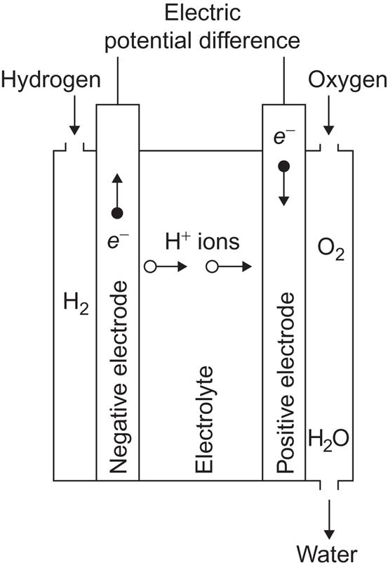
Figure 4.104 shows an example of a fuel cell, based on the free energy change ΔG=−7.9×10⁻¹⁹ J for the reaction
[cf. (3.50)]. Hydrogen gas is led to the negative electrode, which may consist of a porous material, allowing H+ ions to diffuse into the electrolyte, while the electrons enter the electrode material and may flow through the external circuit. If a catalyst (e.g., a platinum film on the electrode surface) is present, the reaction at the negative electrode
(4.144)
may proceed at a much enhanced rate (see, for example, Bockris and Shrinivasan, 1969). Gaseous oxygen (or oxygen-containing air) is similarly led to the positive electrode, where a more complex reaction takes place, the net result of which is
(4.145)
This reaction may be built up by simpler reactions with only two components, such as oxygen first picking up electrons or first associating with a hydrogen ion. A catalyst can also stimulate the reaction at the positive electrode. Instead of porous electrodes, which allow direct contact between the input gases and the electrolyte, membranes can be used (cf. also Bockris and Shrinivasan, 1969), like those found in biological material, i.e., membranes that allow H+ to diffuse through but not H2, etc.
The drop in free energy (4.143) is usually considered mainly associated with reaction (4.145), expressing G in terms of a chemical potential (3.36), e.g., of the H+ ions dissolved in the electrolyte. Writing the chemical potential μ as Faraday’s constant times a potential ϕ, the free energy for n moles of hydrogen ions is
(4.146)
When the hydrogen ions “disappear” at the positive electrode according to reaction (4.145), this chemical free energy is converted into electrical energy (4.142) or (4.143), and, since the numbers of electrons and hydrogen ions in (4.145) are equal, n=ne, the chemical potential μ is given by
(4.147)
Here ϕ is the quantity usually referred to as the electromotive force (e.m.f.) of the cell, or standard reversible potential of the cell, if taken at standard atmospheric pressure and temperature. From the value of ΔG quoted above, corresponding to −2.37×10⁵ J per mole of H2O formed, the cell’s e.m.f. becomes
(4.148)
with n=2 since there are two H+ ions for each molecule of H2O formed. The chemical potential (4.147) may be parametrized in the form (3.37), and the cell e.m.f. may thus be expressed in terms of the properties of the reactants and the electrolyte [including the empirical activity coefficients appearing in (3.37) as a result of generalizing the expression obtained from the definition of the free energy, (4.6), assuming P, V, and T to be related by the ideal gas law, PV=RT, valid for one mole of an ideal gas (cf., for example, Angrist, 1976)].
The efficiency of a fuel cell is the ratio between the electrical power output (4.142) and the total energy lost from the fuel. However, it is possible to exchange heat with the surroundings, and the energy lost from the fuel may thus be different from ΔG. For an ideal (reversible) process, the heat added to the system is
and the efficiency of the ideal process thus becomes
(4.149)
For the hydrogen–oxygen fuel cell considered above, the enthalpy change during the two processes (4.144) and (4.145) is ΔH=−9.5×10⁻¹⁹ J, or −2.86×10⁵ J per mole of H2O formed, and the ideal efficiency is
There are reactions with positive entropy change, such as 2C+O2→2CO, which may be used to cool the surroundings and at the same time create electric power with an ideal efficiency above one (1.24 for CO formation).
In actual fuel cells, a number of factors tend to diminish the power output. They may be expressed in terms of “expenditure” of cell potential fractions on processes not contributing to the external potential,
where each of the terms −ϕi corresponds to a specific loss mechanism. Examples of loss mechanisms are blocking of pores in the porous electrodes [e.g., by piling up of the water formed at the positive electrode in process (4.145)], internal resistance of the cell (heat loss), and the buildup of potential barriers at or near the electrolyte–electrode interfaces. Most of these mechanisms limit the reaction rates and thus tend to place a limit on the current of ions that may flow through the cell. There will be a limiting current, IL, beyond which it will not be possible to draw any more ions through the electrolyte, because of either the finite diffusion constant in the electrolyte, if the ion transport is dominated by diffusion, or the finite effective surface of the electrodes at which the ions are formed. Figure 4.105 illustrates the change in Δϕext as a function of current, expressed as the difference between potential functions at each of the electrodes, Δϕext=ϕc−ϕa. This representation gives some indication of whether the loss mechanisms are connected with the positive or negative electrode processes, and, in this case, the largest fraction of the losses is connected with the more complex positive electrode reactions. For other types of fuel cells, it may be negative ions that travel through the electrolyte, with corresponding changes in characteristics.
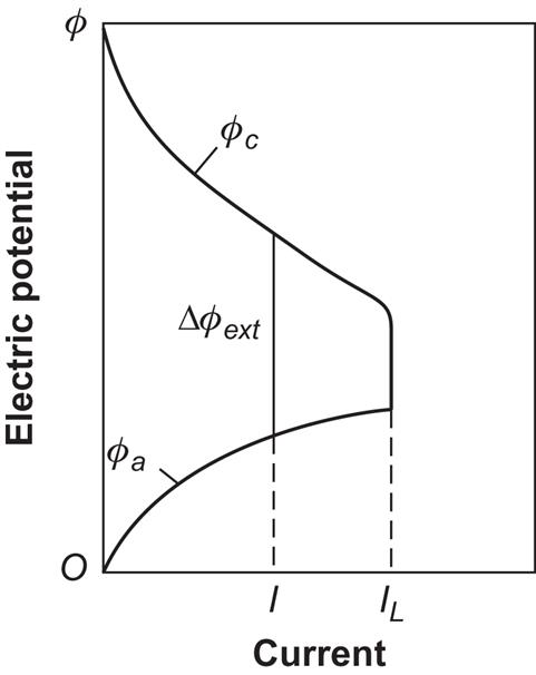
It follows from diagrams of the type in Fig. 4.105 that there will be an optimum current, usually lower than IL, for which the power output will be maximal,
Dividing by the rate at which fuel energy ΔH is added to the system in a steady-state situation maintaining the current Iopt, one obtains the actual efficiency of conversion maximum,
(4.150)
The potential losses within the cell may be described in terms of an internal resistance, the existence of which implies non-zero energy dissipation, if energy is to be extracted in a finite time. This is the same fundamental type of loss as that encountered in solar cells (4.106) and in the general thermodynamic theory described in section 4.1.1.
4.5.1.1 Reverse operation of fuel cells
A driven-cell conversion based on the dissociation of water may be accomplished by electrolysis, using components similar to those of the hydrogen–oxygen fuel cell to perform the inverse reactions. Thus, the efficiency of an ideal conversion may reach 1.20, according to (4.150), implying that the electrolysis process draws heat from the surroundings.
If a fuel cell is combined with an electrolysis unit, a regenerative system is obtained, and if hydrogen and oxygen can be stored, an energy storage system, a battery, results. The electric energy required for the electrolysis need not come from the fuel cell, but may be the result of an intermittent energy conversion process (e.g., wind turbine, solar photovoltaic cell, etc.).
Direct application of radiant energy to the electrodes of an electrochemical cell has been suggested, aiming at the achievement of the driven-cell process (e.g., dissociation of water) without having to supply electric energy. The electrodes could be made of suitable p- and n-type semiconductors, and the presence of photo-induced electron–hole excitations might modify the electrode potentials ϕa and ϕc in such a way that the driven-cell reactions become thermodynamically possible. Owing to the electrochemical losses discussed above, additional energy would have to be provided by solar radiation. Even if the radiation-induced electrode processes have a low efficiency, the overall efficiency may still be higher for photovoltaic conversion of solar energy into electricity followed by conventional electrolysis (Manassen et al., 1976). In recent years, several such photo-electrochemical devices have been constructed. Some of them are described in section 4.4.2. Direct hydrogen production by photo-electrochemical devices is discussed in Sørensen (2012).
4.5.1.2 Fuel-cell design
The idea of converting fuel into electricity by an electrode–electrolyte system originated in the 19th century (Grove, 1839). The basic principle behind a hydrogen–oxygen fuel cell is described above. The first practical applications were in powering space vehicles, starting during the 1970 s. During the late 1990 s, fuel-cell road vehicles were predicted to be ready within a decade, but it did not happen, due to problems with durability and cost. Hybrid vehicles allow a smaller (and thus less costly) fuel cell rating, but if combined with traction batteries the lowering of cost may turn out as difficult as for pure fuel cell vehicles. However, hybrids between either battery electric vehicles or fuel cell vehicles and conventional internal combustion engine vehicles may smooth the transition.
First, hybrids between conventional internal combustion engines and batteries reduce pollution in cities (they use batteries that are charged by the engine at convenient times or that are charged by off-road plug-in power supplies), while using the fuel-based engine for long highway trips will relieve demand on battery size. Second, if and when (presumably) both battery and fuel-cell technologies have come down in cost, the hybrid car could replace the internal combustion engine with a fuel cell plus electric motor, thus allowing total reliance on primary energy from hydrogen or grid electricity, which may both be renewable (see Sørensen, 2006; 2010; 2012).
Fuel technology is described in detail in Sørensen (2012). Here, only some general remarks are made about the development from early fuel-cell concepts to the present-day situation.
Originally developed for stationary power applications, phosphoric acid cells use porous carbon electrodes with a platinum catalyst and phosphoric acid as electrolyte and feed hydrogen to the negative electrode, with electrode reactions given by (4.144) and (4.145). Their operating temperature is 175–200°C, and water is continuously removed.
Alkaline cells use KOH as electrolyte and have electrode reactions of the form
Their operating temperature is 70–100°C, but specific catalysts require maintenance of fairly narrow temperature regimes. Also, the hydrogen fuel must be very pure and, notably, not contain any CO2. Alkaline fuel cells have been used extensively on spacecraft and recently in an isolated attempt for road vehicles (Hoffmann, 1998). Their relative complexity and use of corrosive compounds requiring special care in handling make it unlikely that the cost can be reduced to levels acceptable for general-purpose use.
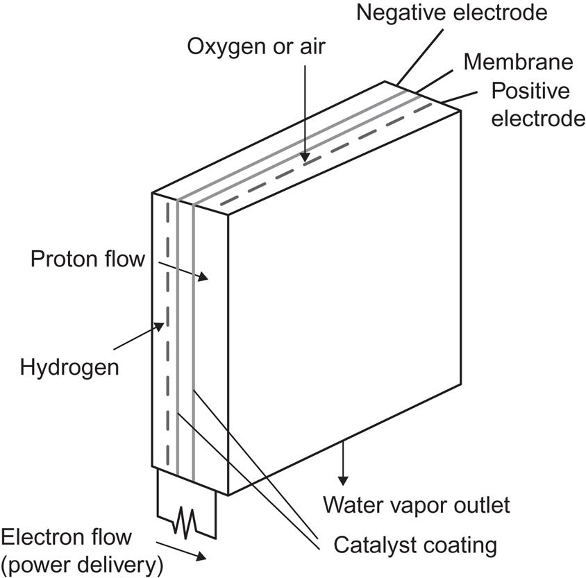
The third fuel cell in commercial use is the proton exchange membrane (PEM) cell. It has been developed over a fairly short period of time and is considered to hold the greatest promise for economic application in the transportation sector. It contains a solid polymer membrane sandwiched between two gas diffusion layers and electrodes. The membrane material may be polyperfluorosulfonic acid. A platinum or Pt–Ru alloy catalyst is used to break hydrogen molecules into atoms at the negative electrode, and the hydrogen atoms are then capable of penetrating the membrane and reaching the positive electrode, where they combine with oxygen to form water, again with the help of a platinum catalyst. The electrode reactions are again (4.144) and (4.145), and the operating temperature is 50–100°C (Wurster, 1997).
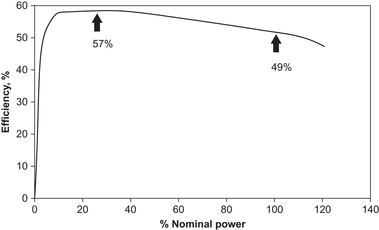
Figure 4.106 shows a typical layout of an individual cell. Several of them are then stacked on top of each other. This modularity implies that PEM cells can be used for applications requiring little power (1 kW or less). PEM cell stacks dominate the current wealth of demonstration projects in road transportation, portable power, and special applications. The efficiency of conversion for small systems is between 30% and 50%, but a 50 kW system has recently shown an efficiency in the laboratory of near 60%. As indicated in Fig. 4.107, an advantage of particular importance for automotive applications is the high efficiency at partial loads, which alone gives a factor of 2 improvement over current internal combustion engines.
For use in automobiles, compressed or liquefied hydrogen is limited by low energy density and safety precautions for containers, but most of all by the requirement for a new infrastructure for fueling. The hydrogen storage problem, which until recently limited fuel-cell projects to large vehicles like buses, may be solved by use of metal hydride or carbon nanofiber stores (see Chapter 5). In order to avoid having to make large changes to gasoline and diesel filling stations, methanol has been proposed as the fuel to be distributed to the vehicle fuel tank. The energy density of methanol is 4.4 kWh liter−1, which is half that of gasoline. This is quite acceptable owing to methanol’s higher efficiency of conversion. Hydrogen is then produced onboard, by a methanol reformer, before being fed to the fuel cell to produce the electric power for an electric motor. The set-up is illustrated in Fig. 4.108. Prototype vehicles with this set-up have been tested (cf. Takahashi, 1998; Brown, 1998), but the reformer technology turned out to have many problems and most current vehicle fuel-cell concepts plan to use hydrogen directly, thereby also avoiding methanol emissions and the health issues connected with the methanol infrastructure.

Methanol, CH3OH, may, however, still find use in fuel-cell development, in a direct methanol PEM fuel cell, without the extra step of reforming to H2. PEM fuel cells that accept a mixture of methanol and water as feedstock have been developed (Bell, 1998) but still have lower energy conversion efficiency than hydrogen-fueled PEM cells. Because methanol can be produced from biomass, hydrogen may be eliminated from the energy system. On the other hand, handling of surplus production of wind or photovoltaic power might still conveniently involve hydrogen as an intermediate energy carrier, since it may have direct uses and thus may improve the system efficiency by avoiding the losses incurred in methanol production. The electric power to hydrogen conversion efficiency is about 65% in high-pressure alkaline electrolysis plants (Wagner et al., 1998; Sørensen, 2012), and the efficiency of the further hydrogen (plus CO or CO2 and a catalyst) to methanol conversion is around 70%. Also, the efficiency of producing methanol from biomass is about 45%, whereas higher efficiencies are obtained if the feedstock is methane (natural gas) (Jensen and Sørensen, 1984; Nielsen and Sørensen, 1998).
For stationary applications, fuel cells of higher efficiency may be achieved by processes operating at higher temperatures. One line of research has been molten carbonate fuel cells, with electrode reactions
The electrolyte is a molten alkaline carbonate mixture retained within a porous aluminate matrix. The carbonate ions formed at the positive electrode travel through the matrix and combine with hydrogen at the negative electrode at an operating temperature of about 650°C. The process was originally aimed at hydrogen supplied from coal gasification or natural gas conversion. Test of a new 250-kW system is taking place at a power utility company in Bielefeld, Germany (Hoffmann, 1998). The expected conversion efficiency is about 55%, and some of the additional high-temperature heat may be utilized. Earlier experiments with molten carbon fuel cells encountered severe problems with material corrosion.
Considerable efforts are being dedicated to solid electrolyte cells. Solid oxide fuel cells (SOFC) use zirconia as the electrolyte layer to conduct oxygen ions formed at the positive electrode. Electrode reactions are
The reaction temperature is 700–1000°C. The lower temperatures are desirable, due to lower corrosion problems, and may be achieved by using a thin electrolyte layer (about 10 μm) of yttrium-stabilized zirconia sprayed onto the negative electrode as a ceramic powder (Kahn, 1996). A number of prototype plants (in the 100-kW size range) are in operation. Current conversion efficiency is about 55%, but it could reach 70–80% in the future (Hoffmann, 1998).
Particularly for vehicle applications of hydrogen-based technologies, efforts are needed to ensure a high level of safety in collisions and other accidents. Because of the difference between the physical properties of hydrogen fuel and the hydrocarbon fuels currently in use (higher diffusion speed, flammability, and explosivity over wider ranges of mixtures with air), there is a need for new safety-related studies, particularly where hydrogen is stored onboard in containers at pressures typically of 20–50 MPa. A few such studies have already been done (Brehm and Mayinger, 1989; see also Sørensen, 2012).
4.5.2 Other electrochemical energy conversion
This chapter describes a number of general principles that have been, or may become, of use in designing actual conversion devices, primarily those aimed at utilizing the renewable flows of energy. Clearly, not all existing or proposed devices have been covered.
The present energy system is dominated by fuels. Solar, wind, and hydro energy bring us away from fuels, but fuels may still play an important role, e.g., in the transport sector. A number of technologies are available to convert fuels among themselves and into electricity and heat or motive power. Many of the technologies can also be used for fuels derived from renewable energy sources. (Fuels derived from biomass are dealt with separately in section 4.6.) For renewable energy sources, such as wind and solar power, one way of dealing with fluctuating production would be to convert surplus electricity to a storable fuel. This could be hydrogen obtained by electrolysis (section 5.3.3 and Sørensen, 2012) or by reversible fuel cells (section 5.3.4). The further conversion of hydrogen to the energy forms in demand can be accomplished by methods already available, for example, for natural gas, such as boilers, engines, gas turbines, and fuel cells.
So far, this chapter describes at least one example of conversion into a useful form of energy for each of the renewable resources described in Chapter 3. This section contains an example of converting more speculative sources of energy, such as the salinity differences identified in section 3.4.3, as renewable energy resources of possible interest.
4.5.2.1 Conversion of ocean salinity gradients
As discussed in section 3.4.3 (Fig. 3.69), a salinity difference like the one existing between fresh (river) and saline (ocean) water, may be used to drive an osmotic pump, and the elevated water may in turn be used to generate electricity by an ordinary turbine (cf. section 4.3.4).
An alternative method, aiming directly at electricity production, takes advantage of the fact that the salts of saline water are ionized to a certain degree and thus may be used to derive an electrochemical cell of the type discussed in section 4.5.1 (Pattie, 1954; Weinstein and Leitz, 1976). Small amounts of power may even be generated by driving an electrolyte through small pores of, e.g., MoS2 by a salinity or pressure gradient (Feng et al., 2016).
The electrochemical cell shown in Fig. 4.109 may be called a dialytic battery, since it is formally the same as the dialysis apparatus producing saline water with electric power input. The membrane allows one kind of ion to pass and thereby reach the corresponding electrode (in contrast to the osmotic pump in Fig. 3.69, where water could penetrate the membrane but ions could not). The free energy difference between the state with free Na+ and Cl− ions (assuming complete ionization) and the state with no such ions is precisely the difference between saline and fresh water, calculated in section 3.4.3 and approximately given by (3.38). Assuming further that each Na+ ion reaching electrode A neutralizes one electron, and that correspondingly each Cl− ion at electrode B gives rise to one electron (which may travel in the external circuit), then the electromotive force, i.e., the electric potential ϕ of the cell, is given in analogy to (4.146), with the number of positive ions per mole equal to ![]() , and ϕ is related to the change in free energy (3.38), just as (4.146) is related to (4.143),
, and ϕ is related to the change in free energy (3.38), just as (4.146) is related to (4.143),
or
(4.151)