
Inserting (5.25) into (5.30), a second-order differential equation for the determination of τr(r) results. The solution depends on materials properties through ρ, Y, and μ and on the state of rotation through ω. Once the radial stress is determined, the tangential one can be evaluated from (5.25).
As an example, consider a plane disc of radius rmax, with a center hole of radius rmin. In this case, the derivatives of b(r) vanish, and the solution to (5.30) and (5.25) is
(5.31)
The radial stress rises from zero at the inner rim, reaches a maximum at r=(rminrmax)1/2, and then declines to zero again at the outer rim. The tangential stress is maximal at the inner rim and declines outward. Its maximum value exceeds the maximum value of the radial stress for most relevant values of the parameters (μ is typically around 0.3).
Comparing (5.25) with (5.16) and the expression for I, it is seen that the energy density W in (5.16) can be obtained by isolating the term proportional to ω2 in (5.25), multiplying it by 1/2r, and integrating over r. The integral of the remaining terms is over a stress component times a shape-dependent expression, and it is customary to use an expression of the form
(5.32)
where M=∫ρb(r)r dθ dr is the total flywheel mass and σ is the maximum stress [cf. (5.18)]. Km is called the shape factor. It depends only on geometry, if all stresses are equal, as in the constant-stress disc, but as the example of a flat disc has indicated [see (5.31)], the material properties and the geometry cannot generally be factorized. Still, the maximum stress occurring in the flywheel may be separated, as in (5.32), in order to leave a dimensionless quantity Km to describe details of the flywheel construction (also, the factor ρ has to be there to balance ρ in the mass M, in order to make Km dimensionless). Expression (5.32) may now be read in the following way: given a maximum acceptable stress σ, there is a maximum energy storage density given by (5.32). It does not depend on ω, and it is largest for light materials and for large design stresses σ. The design stress is typically chosen as a given fraction (safety factor) of the tensile strength. If the tensile strength itself is used in (5.32), the physical upper limit for energy storage is obtained, and using (5.16), the expression gives the maximum value of ω for which the flywheel will not fail by deforming permanently or by disintegrating.
5.5.4 Flywheel performance
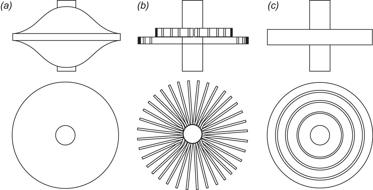
Some examples of flywheel shapes and the corresponding calculated shape factors Km are given in Table 5.6. The infinitely extending disc of constant stress has a theoretical shape factor of unity, but for a practical version with finite truncation, Km of about 0.8 can be expected. A flat, solid disc has a shape factor of 0.6, but if a hole is pierced in the middle, the value reduces to about 0.3. An infinitely thin rim has a shape factor of 0.5 and a finite one, of about 0.4, and a radial rod or a circular brush (cf. Fig. 5.18) has Km equal to one-third.
Table 5.6
| Shape | Km |
| Constant-stress disc | 1 |
| Flat, solid disc (μ=0.3) | 0.606 |
| Flat disc with center hole | ~0.3 |
| Thin rim | 0.5 |
| Radial rod | 1/3 |
| Circular brush | 1/3 |
According to (5.32), the other factors determining the maximum energy density are the maximum stress and the inverse density, in the case of a homogeneous material. Table 5.7 gives tensile strengths and/or design stresses with a safety factor included and gives densities for some materials contemplated for flywheel design.
Table 5.7
Properties of materials considered for flywheels (Davidson et al., 1980; Hagen et al., 1979)
| Material | Density (kg m−3) | Tensile Strength (106 N m−2) | Design Stress (106 N m−2) |
| Birch plywood | 700 | 125 | 30 |
| “Super-paper” | 1100 | 335 | |
| Aluminum alloy | 2700 | 500 | |
| Mild steel | 7800 | 300 | |
| Maraging steel | 8000 | 2700 | 900 |
| Titanium alloy | 4500 | 650 | |
| Carbon fiber (40% epoxy) | 1550 | 1500 | 750 |
| E-glass fiber (40% epoxy) | 1900 | 1100 | 250 |
| S-glass fiber (40% epoxy) | 1900 | 1750 | 350 |
| Kevlar fiber (40% epoxy) | 1400 | 1800 | 1000 |
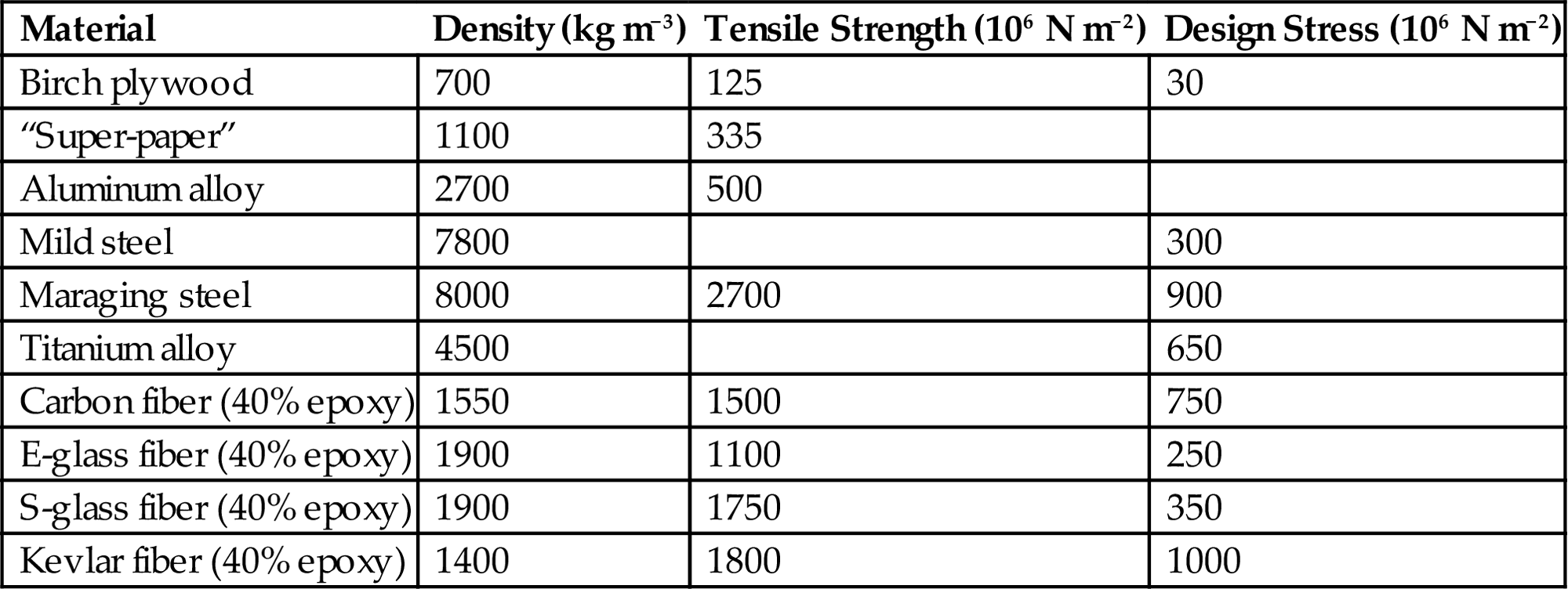
For automotive purposes, the materials with the highest σ/ρ values may be contemplated, although they are also generally the most expensive. For stationary applications, weight and volume are less decisive, and low material cost becomes a key factor. This is the reason for considering cellulosic materials (Hagen et al., 1979). One example is plywood discs, where the disc is assembled from layers of unidirectional plies, each with different orientation. Using (5.32) with the unidirectional strengths, the shape factor should be reduced by a factor of almost 3. Another example in this category is paper-roll flywheels, that is, hollow, cylindrically wound shapes, for which the shape factor is Km=(1+(rmin/rmax)2)/4 (Hagen et al., 1979). The specific energy density would be about 15 kJ kg−1 for the plywood construction and 27 kJ kg−1 for “super-paper” hollow torus shapes.
Unidirectional materials may be used in configurations like the flywheel illustrated in Fig. 5.18b, where tangential (or “hoop”) stresses are absent. Volume efficiency is low (Rabenhorst, 1976). Generally, flywheels made from filament have an advantage in terms of high safety, because disintegration into a large number of individual threads makes a failure easily contained. Solid flywheels may fail by expelling large fragments, and for safety, such flywheels are not proper in vehicles, but may be placed underground for stationary uses.
Approximately constant-stress shapes (cf. Fig. 5.18a) are not as volume efficient as flat discs. Therefore, composite flywheels of the kind shown in Fig. 5.18c have been contemplated (Post and Post, 1973). Concentric flat rings (e.g., made of Kevlar) are separated by elastomers that can eliminate breaking stresses when the rotation creates differential expansion of adjacent rings. Each ring must be made of a different material in order to keep the variations in stress within a small interval. The stress distribution inside each ring can be derived from the expressions in (5.31), assuming that the elastomers fully take care of any interaction between rings. Alternatively, the elastomers can be treated as additional rings, and the proper boundary conditions can be applied (see, for example, Toland, 1975).
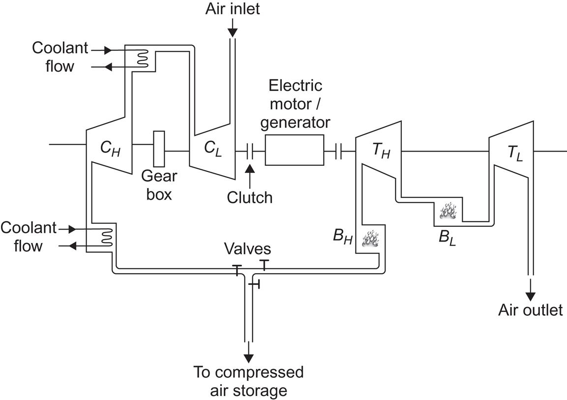
Flywheels of the types described above may attain energy densities of up to 200 kJ kg−1. The problem is to protect this energy against frictional losses. Rotational speeds would typically be 3–5 revolutions per second. The commonly chosen solution is to operate the flywheel in near vacuum and to avoid any kind of mechanical bearings. Magnetic suspension has recently become feasible for units of up to about 200 t, using permanent magnets made from rare-earth cobalt compounds and electromagnetic stabilizers (Millner, 1979). In order to achieve power input and output, a motor generator is inserted between the magnetic bearing suspension and the flywheel rotor. If the motor is placed inside the vacuum, a brushless type is preferable.
For stationary applications, the weight limitations may be circumvented. The flywheel could consist of a horizontally rotating rim wheel of large dimensions and weight, supported by rollers along the rim or by magnetic suspension (Russell and Chew, 1981; Schlieben, 1975). Energy densities of about 3000 kJ kg−1 could, in principle, be achieved by using fused silica composites (cf. fibers of Table 5.7). The installations would then be placed underground in order to allow reduced safety margins. Unit sizes could be up to 105 kg.
5.5.5 Compressed gas storage
Gases tend to be much more compressible than solids or fluids, and investigations of energy storage applications of elastic energy on a larger scale have therefore concentrated on the use of gaseous storage media.
Storage on a smaller scale may make use of steel containers, such as the ones common for the compressed air used in mobile construction work. In this case, the volume is fixed and the amount of energy stored in the volume is determined by the temperature and the pressure. If air is treated as an ideal gas, the (thermodynamic) pressure P and temperature T are related by the equation of state
(5.33)
where V is the volume occupied by the air, ν is the number of moles in the volume, and ℜ=8.315 J K−1 mol−1. The pressure P corresponds to the stress in the direction of compression for an elastic cube, except that the sign is reversed (in general, the stress equals –P plus viscosity-dependent terms). The container may be thought of as a cylinder with a piston enclosing a given number of moles of gas, say, air. The compressed air is formed by compressing the enclosed air from standard pressure at the temperature of the surroundings, that is, increasing the force fx applied to the piston, while the volume decreases from V0 to V. The amount of energy stored is
(5.34)
where A is the cylinder cross-sectional area, x and x0 are the piston positions corresponding to V and V0, and P is the pressure of the enclosed air.
For large-scale storage applications, underground cavities have been considered. The three possibilities investigated until now are salt domes, cavities in solid rock formations, and aquifers.
Cavities in salt deposits may be formed by flushing water through the salt. The process has, in practical cases, been extended over a few years, in which case the energy spent (and cost) has been very low (Weber, 1975). Salt domes are salt deposits extruding upward toward the surface, therefore allowing cavities to be formed at modest depths.
Rock cavities may be either natural or excavated, and the walls are properly sealed to ensure air-tightness. If excavated, they are much more expensive to make than salt caverns.
Aquifers are layers of high permeability, permitting underground water flows along the layer. In order to confine the water stream to the aquifer, there have to be encapsulating layers of little or no permeability above and below the water-carrying layer. Aquifers usually do not stay at a fixed depth, and thus, they can have slightly elevated regions where a certain amount of air can become trapped without impeding the flow of water. This possibility for air storage (under the elevated pressure corresponding to the depth involved) is illustrated in Fig. 5.19c.
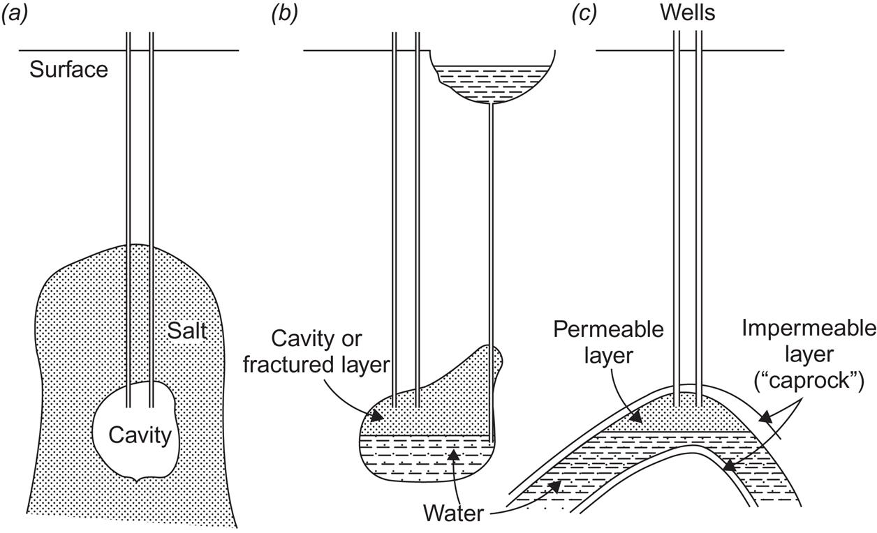
Figure 5.19 illustrates the forms of underground air storage mentioned: salt, rock, and aquifer storage. In all cases, site selection and preparation are a fairly delicate process. Although the general geology of the area considered is known, the detailed properties of the cavity will not become fully known until the installation is complete. The ability of the salt cavern to keep an elevated pressure may not live up to expectations based on sample analysis and pressure tests at partial excavation. The stability of a natural rock cave, or of a fractured zone created by explosion or hydraulic methods, is also uncertain until actual full-scale pressure tests have been conducted. For aquifers, decisive measurements of permeability can be made at only a finite number of places, so surprises are possible due to rapid permeability change over small distances of displacement (cf. Adolfson et al., 1979).
The stability of a given cavern is influenced by two design features that operation of the compressed air storage system will entail: notably temperature and pressure variations. It is possible to keep the cavern wall temperature nearly constant, either by cooling the compressed air before letting it down into the cavern or by performing the compression so slowly that the temperature rises only to the level prevailing on the cavern walls. The latter possibility (isothermal compression) is impractical for most applications, because excess power must be converted at the rate at which it is produced. Most systems, therefore, include one or more cooling steps. With respect to the problem of pressure variations, when different amounts of energy are stored, the solution may be to store the compressed air at constant pressure but variable volume. In this case, either the storage volume itself should be variable, as it is with aquifer storage (when variable amounts of water are displaced), or the underground cavern should be connected to an open reservoir (Fig. 5.19b), so that a variable water column may respond to the variable amounts of air stored at the constant equilibrium pressure prevailing at the depth of the cavern. This kind of compressed energy storage system may alternatively be viewed as a pumped hydro storage system, with extraction taking place through air-driven turbines rather than through water-driven turbines.
5.5.6 Adiabatic storage
Consider now the operation of a variable-pressure system. The compression of ambient air takes place approximately as an adiabatic process, that is, without heat exchange with the surroundings. If γ denotes the ratio between the partial derivatives of pressure with respect to volume at constant entropy and at constant temperature,
(5.35)
and the ideal gas law (5.33) gives (∂ P/∂ V)T=– P/V, so that for constant γ,
(5.36)
The constant on the right-hand side is here expressed in terms of the pressure P0 and volume V0 at a given time. For air at ambient pressure and temperature, γ=1.40. The value decreases with increasing temperature and increases with increasing pressure, so (5.36) is not entirely valid for air. However, in the temperature and pressure intervals relevant for practical application of compressed air storage, the value of γ varies less than ±10% from its average value.
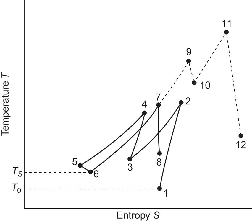
Inserting (5.36) into (5.34), we get the amount of energy stored,
(5.37)
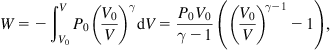 (5.37)
or, alternatively,
(5.38)
 (5.38)
More precisely, this is the work required for the adiabatic compression of the initial volume of air. This process heats the air from its initial temperature T0 to a temperature T, which can be found by rewriting (5.33) in the form
and combining it with the adiabatic condition (5.36),
(5.39)
Since desirable pressure ratios in practical applications may be up to about P/P0=70, maximum temperatures exceeding 1000 K can be expected. Such temperature changes would be unacceptable for most types of cavities considered, and the air is therefore cooled before transmission to the cavity. Surrounding temperatures for underground storage are typically about 300 K for salt domes and somewhat higher for storage in deeper geological formations. With this temperature denoted as Ts, the heat removed if the air is cooled to Ts at constant pressure amounts to
(5.40)
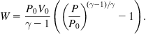
where cP is the heat capacity at constant pressure. Ideally, the heat removed would be kept in a well-insulated thermal energy store, so that it can be used to reheat the air when it is taken up from the cavity to perform work by expansion in a turbine, with the associated pressure drop back to ambient pressure P0. Viewed as a thermodynamic process in a temperature–entropy (T, S)-diagram, the storage and retrieval processes in the ideal case are as shown in Fig. 5.20. The process leads back to its point of departure, indicating that the storage cycle is loss-free under the idealized conditions assumed so far.
In practice, the compressor has a loss (of maybe 5%–10%), meaning that not all the energy input (electricity, mechanical energy) is used to perform compression work on the air. Some is lost as friction heat, and so on. Furthermore, not all the heat removed by the cooling process can be delivered to reheat the air. Heat exchangers have finite temperature gradients, and there may be losses from the thermal energy store during the time interval between cooling and reheating. Finally, the exhaust air from actual turbines has temperatures and pressures above ambient. Typical loss fractions in the turbine may be around 20% of the energy input, at the pressure considered above (70 times ambient) (Davidson et al., 1980). If less than 10% thermal losses could be achieved, the overall storage cycle efficiency would be about 65%.
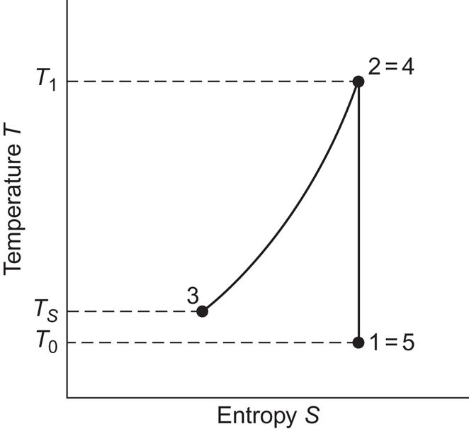
The real process may proceed as shown in Fig. 5.21, as function of temperature and entropy changes. The compressor loss in the initial process 1-2 modifies the vertical line to include an entropy increase. Furthermore, compression has been divided into two steps (1-2 and 3-4) in order to reduce the maximum temperatures. Correspondingly, there are two cooling steps (2-3 and 4-5), followed by a slight final cooling performed by the cavity surroundings (5-6). The work-retrieval process involves, in this case, a single step 6-7 of reheating by use of heat stored from the cooling processes (in some cases, more than one reheating step is employed). Finally, 7-8 is the turbine stage, which leaves the cycle open by not having the air reach the initial temperature (and pressure) before it leaves the turbine and mixes into the ambient atmosphere. In addition, this expansion step shows deviations from adiabaticity, seen in Fig. 5.21 as an entropy increase.
There are currently only a few utility-integrated installations. The earliest full-scale compressed storage facility has operated since 1978 at Huntorf, Germany. It is rated at 290 MW and has about 3×10⁵ m3 storage volume (Lehmann, 1981). It does not have any heat recuperation, but it has two fuel-based turbine stages, implying that the final expansion takes place from a temperature higher than any of those involved in the compression stages (and also at higher pressure). This is indicated in Fig. 5.21 as 7-9-10-11-12, where steps 7-9 and 10-11 represent additional heating based on fuel, while steps 9-10 and 11-12 indicate expansion through turbines. If heat recuperation is added, as it is in the 110 MW plant operated by the Alabama Electric Corp. (USA) since 1991, point 7 moves upward toward point 9, and point 8 moves in the direction of 12, altogether representing an increased turbine output (Linden, 2003).
The efficiency calculation is changed in the case of additional fuel combustion. The additional heat input may be described by (5.40) with appropriate temperatures substituted, and the primary enthalpy input H0 is obtained by dividing H by the fuel-to-heat conversion efficiency. In the case of a finite compressor efficiency ηc, the input work Win to the compressor changes from (5.38) to
(5.41)
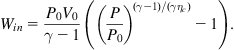 (5.41)
The work delivered by the turbine receiving air of pressure P1 and volume V1, and exhausting it at P2 and V2, with a finite turbine efficiency ηt, is
(5.42)
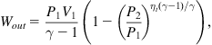 (5.42)
which, except for the appearance of ηt, is just (5.38) rewritten for the appropriate pressures and volume.
When there is only a single compressor and a single turbine stage, the overall cycle efficiency is given by
(5.43)
For the Huntorf compressed air storage installation, η is 0.41. Of course, if the work input to the compressor is derived from fuel (directly or through electricity), Win may be replaced by the fuel input W0 and a fuel efficiency defined as
(5.44)
If Win/W0 is taken as 0.36, ηfuel for the example becomes 0.25, which is 71% of the conversion efficiency for electric power production without going through the store. The German installation is used for providing peak power on weekdays, and is charged during nights and weekends.
Figure 5.22 shows the physical layout of the German plant, and Fig. 5.23 shows the layout of a more advanced installation with no fuel input, corresponding to the two paths illustrated in Fig. 5.21.

5.5.7 Aquifer storage
The aquifer storage system shown in Fig. 5.19c would have an approximately constant working pressure, corresponding to the average hydraulic pressure at the depth of the air-filled part of the aquifer. According to (5.34), the stored energy in this case simply equals the pressure P times the volume of air displacing water in the aquifer. This volume equals the physical volume V times the porosity p, that is, the fractional void volume accessible to intruding air (there may be additional voids that the incoming air cannot reach), so the energy stored may be written
(5.45)
Typical values are p=0.2 and P around 6×10⁶ N m−2 at depths of about 600 m, with useful volumes of 109 to 1010 m3 for each site. Several such sites have been investigated for the possible storage of natural gas.
An important feature of an energy storage aquifer is the time required for charging and emptying. This time is determined by the permeability of the aquifer. The permeability is basically the proportionality factor between the flow velocity of a fluid or gas through the sediment and the pressure gradient causing the flow. The linear relationship assumed may be written
(5.46)
where ν is the flow velocity, η is the viscosity of the fluid or gas, ρ is its density, P is the pressure, and s is the path-length in the downward direction. K is the permeability, being defined by (5.46). In metric (SI) units, the unit of permeability is m2. The unit of viscosity is m2 s−1. Another commonly used unit of permeability is the darcy. One darcy equals 1.013×10¹² m2. If filling and emptying of the aquifer storage are to take place in a matter of hours, rather than days, permeability has to exceed 1011 m2. Sediments, such as sandstone, have permeabilities ranging from 1010 to 3×10¹² m2, often with considerable variation over short distances.
In actual installations, losses occur. The cap-rock bordering the aquifer region may not have negligible permeability, implying a possible leakage loss. Friction in the pipes leading to and from the aquifer may cause a loss of pressure, as may losses in the compressor and turbine. Typically, losses of about 15% are expected in addition to those of the power machinery. Large aquifer stores for natural gas are in operation: the store at Stenlille, Denmark has 109 m3 total volume, from which 3.5×10⁸ m3 of gas can be extracted at the employed pressure of 17 MPa (DONG, 2003). The same gas utility company built an excavated salt dome gas storage at Lille Thorup that has a slightly smaller volume but allows 4.2×10⁸ m3 of gas to be extracted at 23 MPa.
5.5.7.1 Hydrogen storage
Hydrogen can be stored like other gases, compressed in suitable containers capable of managing the high diffusivity of hydrogen, as well as sustaining the pressures required to bring the energy density up to useful levels. However, the low energy density of gaseous hydrogen has brought alternative storage forms into the focus of investigation, such as liquid hydrogen and hydrogen trapped inside metal hydride structures or inside carbon-based or other types of nanotubes (cf. Sørensen, 2012).
Hydrogen is an energy carrier, not a primary energy form. The storage cycle therefore involves both the production of hydrogen from primary energy sources and the retrieval of the energy form demanded by a second conversion process.
5.5.8 Hydrogen production
Conventional hydrogen production is by catalytic steam-reforming of methane (natural gas) or gasoline with water vapor. The process, which typically takes place at 850°C and 2.5×10⁶ Pa, is
(5.47)
followed by the catalytic shift reaction
(5.48)
Finally, CO2 is removed by absorption or membrane separation. The heat produced by (5.48) often cannot be directly used for (5.47). For heavy hydrocarbons, including coal dust, a partial oxidation process is currently in use (Zittel and Wurster, 1996). An emerging technology is high-temperature plasma-arc gasification, and a pilot plant based on this technology operates on natural gas at 1600°C in Norway (at Kvaerner Engineering). The advantage of this process is the pureness of the resulting products (in energy terms, 48% hydrogen, 40% carbon, and 10% water vapor) and therefore low environmental impact. Since all the three main products are useful energy carriers, the conversion efficiency may be said to be 98% minus the energy needed for the process.
However, conversion of natural gas to carbon is not normally desirable, and the steam can be used only locally, so 48% efficiency is more meaningful.
Production of hydrogen from biomass may be achieved by biological fermentation or by high-temperature gasification similar to that used for coal. These processes are described in more detail in section 4.6.2. Production of hydrogen from (wind- or solar-produced) electricity may be achieved by conventional electrolysis (demonstrated by Faraday in 1820 and widely used since about 1890) or by reversible fuel cells, with current efficiencies of about 70% and over 90%, respectively.
Electrolysis conventionally uses an aqueous alkaline electrolyte, with the anode and cathode areas separated by a microporous diaphragm (replacing earlier asbestos diaphragms), so that
(5.49)
(5.50)
At 25°C, the change in free energy, ΔG, is 236 kJ mol−1, and electrolysis would require a minimum amount of electric energy of 236 kJ mol−1, while the difference between enthalpy and free energy changes, ΔH − ΔG, in theory could be heat from the surroundings. The energy content of hydrogen (equal to ΔH) is 242 kJ mol−1 (lower heating value), so T ΔS could exceed 100%. However, if heat is added at 25°C, the process is exceedingly slow. Temperatures used in actual installations are so high that the heat balance is positive and cooling has to be applied. This is largely a consequence of electrode overvoltage, mainly stemming from polarization effects. The cell potential V for water electrolysis may be expressed by
(5.51)
where Vr is the reversible cell potential. The overvoltage has been divided into the anodic and cathodic parts Va and Vc. The current is j, and R is the internal resistance of the cell. The last three terms in (5.51) represent the electrical losses, and the voltage efficiency ηV of an electrolyzer operating at a current j is given by
(5.52)
while the thermal efficiency is
(5.53)
with the Faraday constant being ![]() =96 493 coulombs mol−1, and n being the number of moles transferred in the course of the overall electrochemical reaction to which ΔG relates.
=96 493 coulombs mol−1, and n being the number of moles transferred in the course of the overall electrochemical reaction to which ΔG relates.
Efforts are being made to increase the efficiency above the current 50% to 80% (for small to large electrolyzers) by increasing the operating temperature and optimizing electrode materials and cell design; in that case, the additional costs should be less than for the emerging solid-state electrolyzers, which are essentially fuel cells operated in reverse, i.e., using electric power to produce hydrogen and oxygen from water in an arrangement and with reaction schemes formally the same as those of the fuel cells described in section 4.5. If the same fuel cell allows operation in both directions, it is called a reversible fuel cell.
A third route contemplated for hydrogen production from water is thermal decomposition of water. Because direct thermal decomposition of water molecules requires temperatures exceeding 3000 K, which is not possible with presently available materials, attempts have been made to achieve decomposition below 800°C by an indirect route using cyclic chemical processes. Such thermochemical or water-splitting cycles were originally designed to reduce the required temperature to the low values attained in nuclear reactors, but could, of course, be used with other technologies generating heat at around 400°C. An example of the processes studied (Marchetti, 1973) is the three-stage reaction
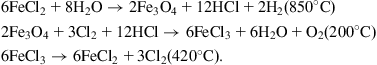
The first reaction still requires a high temperature, implying a need for energy to be supplied, in addition to the problem of the corrosive substances involved. Researchers are still a long way from creating a practical technology.
The process of water photodissociation is described in section 3.5.1. There have been several attempts to imitate the natural photosynthetic process, using semiconductor materials and membranes to separate the hydrogen and oxygen formed by application of light (Calvin, 1974; Wrighton et al., 1977). So far, no viable reaction scheme has been found, either for artificial photodissociation or for hybrid processes using heat and chemical reactions in side processes (Hagenmuller, 1977).
Processing of the hydrogen produced involves removal of dust and sulfur, as well as other impurities, depending on the source material (e.g., CO2 if biogas is the source).
5.5.9 Hydrogen storage forms
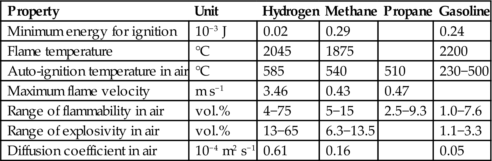
The storage forms relevant for hydrogen are connected with its physical properties, such as the energy density shown in Table 5.5 for hydrogen in various forms. Combustion and safety-related properties are shown in Table 5.8 and are compared with those of methane, propane, and gasoline. Hydrogen’s high diffusivity has implications for container structure, and hydrogen has a large range of flammability/explosivity to consider in all applications.
Table 5.8
Safety-related properties of hydrogen and other fuels (with use of Zittel and Wurster, 1996)
| Property | Unit | Hydrogen | Methane | Propane | Gasoline |
| Minimum energy for ignition | 10−3 J | 0.02 | 0.29 | 0.24 | |
| Flame temperature | °C | 2045 | 1875 | 2200 | |
| Auto-ignition temperature in air | °C | 585 | 540 | 510 | 230−500 |
| Maximum flame velocity | m s−1 | 3.46 | 0.43 | 0.47 | |
| Range of flammability in air | vol.% | 4−75 | 5−15 | 2.5−9.3 | 1.0−7.6 |
| Range of explosivity in air | vol.% | 13−65 | 6.3−13.5 | 1.1−3.3 | |
| Diffusion coefficient in air | 10−4 m2 s−1 | 0.61 | 0.16 | 0.05 |
5.5.9.1 Compressed storage in gaseous form
The low volume density of hydrogen at ambient pressure (Table 5.5) makes compression necessary for energy storage applications. Commercial hydrogen containers presently use pressures of 20–30×106 Pa, with corresponding energy densities of 1900−2700×106 J m−3, which is still less than 10% of that of oil. Research is in progress for increasing pressures to about 70 MPa, using high-strength composite materials such as Kevlar fibers. Inside liners of carbon fibers (earlier, glass/aluminum was used) are required to reduce permeability. Compression energy requirements influence storage-cycle efficiencies and involve long transfer times. The work required for isothermal compression from pressure p1 to p2 is of the form
where A is the hydrogen gas constant 4124 J K−1 kg−1 times an empirical, pressure-dependent correction (Zittel and Wurster, 1996). To achieve compression, a motor rated at Bm must be used, where m is the maximum power throughput and B, depending on engine efficiency, is around 2.
5.5.9.2 Liquid hydrogen stores
Because the liquefaction temperature of hydrogen is 20 K (−253°C), the infrastructure and energy requirements for liquefaction are substantial (containers and transfer pipes must be superinsulated). On the other hand, transfer times are low (currently 3 min to charge a passenger car). The energy density is still 4–5 times lower than for conventional fuels (see Table 5.5). The liquefaction process requires very clean hydrogen, as well as several cycles of compression, liquid nitrogen cooling, and expansion.
5.5.9.3 Metal hydride storage
Hydrogen diffused into appropriate metal alloys can achieve storage at volume densities over two times that of liquid hydrogen. However, the mass storage densities are still less than 10% of those of conventional fuels (Table 5.5), making this concept doubtful for mobile applications, despite the positive aspects of nearly loss-free storage at ambient pressures (0–6 MPa) and transfer accomplished by adding or withdrawing modest amounts of heat (associated with high safety in operation), according to
(5.54)
where the hydride may be body-centered cubic lattice structures with about 6×1028 atoms per m3 (such as LaNi5H6, FeTiH2). The currently highest density achieved is for metal alloys absorbing two hydrogen atoms per metal atom (Toyota, 1996). The lattice absorption cycle also cleans the gas, because impurities in the hydrogen gas are too large to enter the lattice.
5.5.9.4 Methanol storage
One current prototype hydrogen-fueled vehicle uses methanol as storage, even if the desired form is hydrogen (because the car uses a hydrogen fuel cell to generate electricity for its electric motor; Daimler-Chrysler-Ballard, 1998). The reason is the simplicity of the methanol storage and filling infrastructure. In the long run, transformation of hydrogen to methanol and back seems too inefficient, and it is likely that the methanol concept will be combined with methanol fuel cells (cf. section 4.7), while hydrogen-fueled vehicles must find simpler storage alternatives.
5.5.9.5 Graphite nanofiber stores
Current development of nanofibers has suggested wide engineering possibilities for both electric and structural adaptation, including the storage of foreign atoms inside “balls” or “tubes” of large carbon structures (Zhang et al., 1998). Indications are that hydrogen may be stored in nanotubes in quantities exceeding the capacity of metal hydrides, and at a lower weight penalty, but no designs exist yet (Service, 1998).
5.5.10 Regeneration of power from hydrogen
Retrieval of energy from stored hydrogen may be by conventional low-efficiency combustion in Otto engines or gas turbines, or it may be through fuel cells at a considerably higher efficiency, as described in section 4.7 and in Sørensen (2012).
5.5.11 Battery storage
Batteries may be described as fuel cells where the fuels are stored inside the cell rather than outside it. Historically, batteries were the first controlled source of electricity, with important designs being developed in the early 19th century by Galvani, Volta, and Daniell, before Grove’s discovery of the fuel cell and Planté’s construction of the lead–acid battery. Today, available batteries use a wide range of electrode materials and electrolytes, but, despite considerable development efforts aimed at the electric utility sector, in practice battery storage is still restricted to small-scale use (consumer electronics, motor cars, etc.).
Efforts are being made to find systems with better performance than the long-employed lead–acid batteries, which are restricted by a low energy density (see Table 5.5) and a limited life. Alkaline batteries, such as nickel–cadmium cells, proposed around 1900 but first commercialized during the 1970s, are the second largest market for use in consumer electronics and, recently, in electric vehicles. Despite their high cost, lithium-ion batteries have had a rapid impact since their introduction in 1991 (see below). They allow charge topping (i.e., charging before complete discharge) and have a high energy density, suitable for small-scale portable electronic equipment.
Rechargeable batteries are called accumulators or secondary batteries, whereas use-once-only piles are termed primary batteries. Table 5.9 gives some important characteristics of various battery types. The research goals set in 1977 for high-power batteries have been reached in commercially available products, but the goals for high-energy-density cells have not quite been reached. One reason for the continued high market share of lead–acid batteries is the perfection of this technology that took place over the last decades.
Table 5.9
Characteristics of selected batteries (Jensen and Sørensen, 1984; Cultu, 1989; Scrosati, 1995; Buchmann, 1998) and comparison with 1977 development goals (Weiner, 1977)
| Type | Electrolyte | Energy Efficiency (%) | Energy Density (Wh kg−1) | Power Densities | Cycle Life (Cycles) | Operating Temperatures (°C) | |
| Peak (W kg−1) | Sustained (W kg−1) | ||||||
| Commercial | |||||||
| Lead–acid | H2SO4 | 75 | 20−35 | 120 | 25 | 200−2000 | −20 to 60 |
| Nickel–cadmium | KOH | 60 | 40−60 | 300 | 140 | 500–2000 | −40 to 60 |
| Nickel–metal-hydride | KOH | 50 | 60−80 | 440 | 220 | <3000 | 10 to 50 |
| Lithium-ion | LiPF6 | 70 | 100−200 | 720 | 360 | 500−2000 | −20 to 60 |
| Under development | |||||||
| Sodium–sulfur | β-Al2O3 | 70 | 120 | 240 | 120 | 2000 | 300 to 400 |
| Lithium–sulfide | AlN | 75 | 130 | 200 | 140 | 200 | 430 to 500 |
| Zinc–chlorine | ZnCl2 | 65 | 120 | 100 | 0 | ||
| Lithium–polymer | Li–β-Alu | 70 | 200 | >1200 | −20 to 60 | ||
| 1977 goal cells | |||||||
| High energy | 65 | 265 | 55–100 | 2500 | |||
| High power | 70 | 60 | 280 | 140 | 1000 | ||

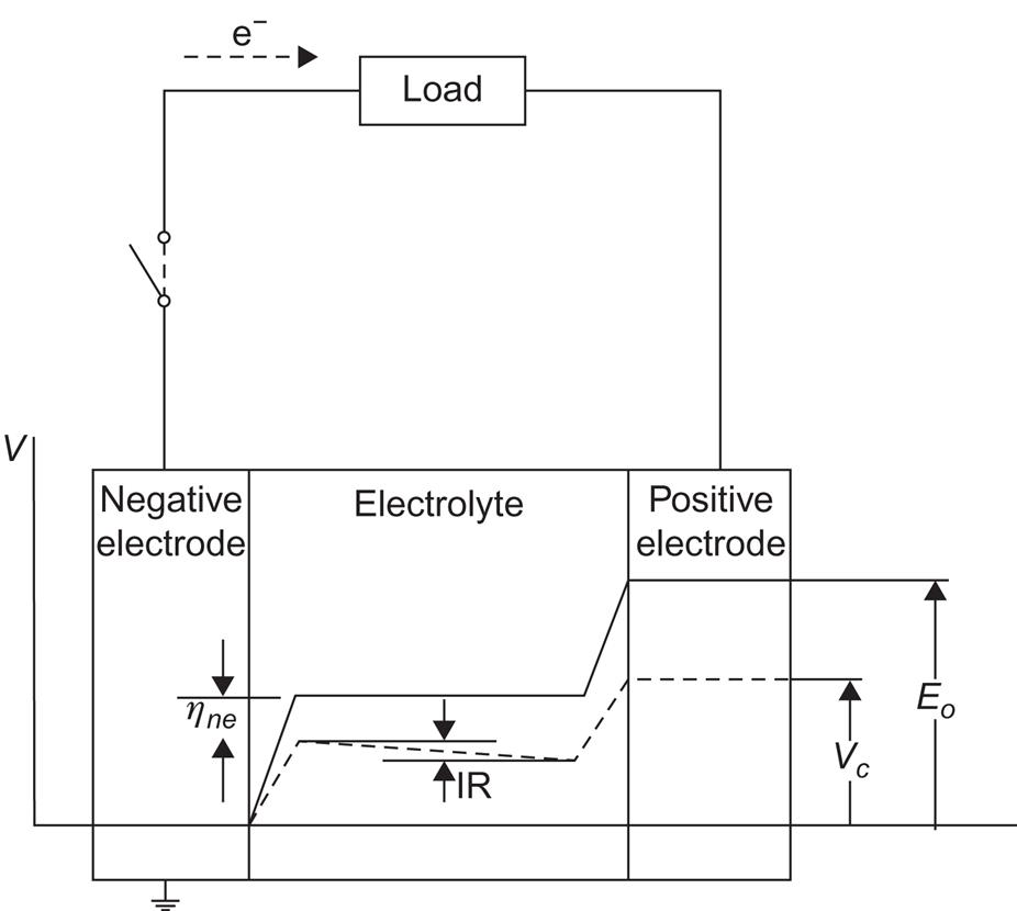
An electrochemical storage battery has properties determined by cell voltage, current, and time constants. The two electrodes delivering or receiving power to or from the outside are called en and ep (negative and positive electrode). (The conventional terms anode and cathode are confusing in the case of rechargeable batteries.) Within the battery, ions are transported between the negative and positive electrodes through an electrolyte. This, as well as the electrodes, may be solid, liquid, or, in theory, gaseous. The electromotive force E0 is the difference between the electrode potentials for an open external circuit,
(5.55)
where it is customary to measure all potentials relative to some reference state. The description of open-cell behavior uses standard steady-state chemical reaction kinetics. However, when current flows to or from the cell, equilibrium thermodynamics is no longer applicable, and the cell voltage Vc is often parametrized in the form
(5.56)
where I is the current at a given time, R is the internal resistance of the cell, and η is a “polarization factor” receiving contributions from the possibly very complex processes taking place in the transition layer separating each electrode from the electrolyte. Figure 5.24 illustrates the different potential levels across the cell for open and closed external circuits (cf., for example, Bockris and Reddy, 1973).
5.5.11.1 The lead–acid battery
In the electrolyte (aqueous solution of sulfuric acid) of a lead–acid battery, three reactions are at work,
(5.57)
 (5.57)
and at the (lead and lead oxide) electrodes, the reactions are
(5.58)
The electrolyte reactions involve ionization of water and either single- or double-ionization of sulfuric acid. At both electrodes, lead sulfate is formed, from lead oxide at the positive electrode and from lead itself at the negative electrode. Developments have included sealed casing, thin-tube electrode structure, and electrolyte circulation. As a result, the internal resistance has been reduced, and the battery has become practically maintenance-free throughout its life. The energy density of the lead–acid battery increases with temperature and decreases with discharge rate (by about 25% when going from 10 to 1 h discharge, and by about 75% when going from 1 h to 5 min discharge; cf. Jensen and Sørensen, 1984). The figures given in Table 5.9 correspond to an average discharge rate and an 80% depth of discharge.
While flat-plate electrode-grid designs are still in use for automobile starter batteries, tubular-plate designs have a highly increased cycle life and are used for electric vehicles and increasingly for other purposes. The projected life of tubular-plate batteries is about 30 years, according to enhanced test cycling. Charging procedures for lead–acid batteries influence battery life.
5.5.11.2 Alkaline electrolyte batteries
Among the alkaline electrolyte batteries, nickel–cadmium batteries, which have been used since about 1910, were based upon investigations during the 1890s by Jungner. Their advantage is a long lifetime (up to about 2000 cycles) and, with careful use, a nearly constant performance, independent of discharge rate and age (Jensen and Sørensen, 1984). However, they do not allow drip charging and easily drop to low capacity if proper procedures are not followed. During the period 1970–1990, they experienced an expanding penetration in applications for powering consumer products, such as video cameras, cellular phones, portable players, and portable computers, but they have now lost most of these markets to the more expensive lithium-ion batteries.
Iron–nickel oxide batteries, which were used extensively in the early part of the 20th century in electric motorcars, have inferior cell efficiency and peaking capability, owing to their low cell voltage and high internal resistance, which also increases the tendency for self-discharge. Alternatives, such as nickel–zinc batteries, are hampered by low cycle life.
The overall reaction for NiCd batteries may be summarized as
(5.59)
The range of cycle lives indicated in Table 5.9 reflects the sensitivity of NiCd batteries to proper maintenance, including frequent deep discharge. For some applications, it is not practical to have to run the battery down to zero output before recharging.
An alternative considered is nickel–metal hydride batteries, which exhibit a slightly higher energy density but so far have a shorter cycle life.
5.5.11.3 High-temperature batteries
Research on high-temperature batteries for electric utility use (cf. Table 5.9) has been ongoing for several decades, without decisive breakthroughs. Their advantage would be fast, reversible chemistry, allowing for high current density without excess heat generation. Drawbacks include serious corrosion problems, which have persisted and have curtailed the otherwise promising development of, for example, the sodium–sulfur battery. This battery has molten electrodes and a solid electrolyte; it is usually of tubular shape and is made from ceramic beta-alumina materials. Similar containment problems have affected zinc–chlorine and lithium–sulfur batteries.
5.5.11.4 Lithium-ion batteries
Lithium metal electrode batteries attracted attention several decades ago (Murphy and Christian, 1979), owing to their potentially very high energy density. However, explosion risks delayed commercial applications until the lithium-ion concept was developed by Sony in Japan (Nagaura, 1990). Its electrode materials are LiCoO2 and LixC6 (carbon or graphite), respectively, with an electrolyte of lithium hexafluorophosphate dissolved in a mixture of ethylene carbonate and dimethylcarbonate (Scrosati, 1995). The battery is built from alternating layers of electrode materials, between which the lithium ions oscillate cyclically (Fig. 5.25). The cell potential is high, 3.6 or 7.2 V. Lithium-ion batteries do not accept overcharge, and a safety device is usually integrated in the design to provide automatic venting in case of emergency. Owing to its high power density (by weight or volume) and easy charging (topping up is possible without loss of performance), the lithium-ion battery has rapidly penetrated to the high-end portable equipment sector. Its safety record is excellent, justifying abandoning the lithium metal electrode, despite some loss of power. The remaining environmental concern is mainly the use of cobalt, which is very toxic and requires an extremely high degree of recycling to be acceptable. With time, cost has declined and Li-ion batteries are currently used on an intermediate scale, in garden equipment, craftsman tools and electric vehicles, from bicycles and wheelchairs to cars and buses. Applications for bulk power storage in dealing with the intermittency of several renewable energy systems is still awaiting further technology development to reduce cost and environmental risks (Sørensen, 2015).

Ongoing research on lithium-ion batteries aims at bringing the price further down and avoiding the use of cobalt, while maintaining the high level of safety and possibly improving performance. The preferred concept uses an all-solid-state structure with lithium–beta–alumina forming a layered electrolyte and LiMn2O4 or LiMnO2 as the positive electrode material (Armstrong and Bruce, 1996). The reaction at the positive electrode belongs to the family of intercalation reactions (Ceder et al., 1998),
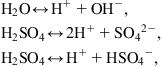
Other ideas include use of lithium–polymer batteries. Currently, the ionic conductivity of solid polymer materials is too low to allow ambient temperature operation, but operating temperatures of around 80°C should be acceptable for non-portable applications (Tarascon and Armand, 2001). After several years of research, lithium–oxygen or lithium–air batteries have now shown properties considered promising (Ogasawara et al., 2006; Armand and Tarascon, 2008; Lu et al., 2016). Fig. 5.26 shows the layout of a Li2O2 battery using a MnO2 nanowire as catalyst (Débart et al., 2008). Many other rechargeable battery configurations have been researched for decades, such as aluminum-ion batteries offering low flammability, but degradation and other problems have so far prevented industrial development (Lin et al., 2015).
Mandatory recycling of batteries has already been introduced in several countries and is clearly a must for some of the recently emerging battery designs.
Currently, lithium-ion batteries are being used in devices requiring larger and larger storage capacity, from vacuum cleaners and garden equipment to electric bicycles and cars. Electric road vehicles may finally have reached the point of being a realistic bid for a zero-emission technology.
If batteries ever get to the point of being suitable for use in the grid-based electricity supply sector, it is likely to be for short-term and medium-term storage. Batteries have already been extensively incorporated into off-grid systems, such as rural power systems (whether based upon renewable energy or diesel sets) and stand-alone systems, such as security back-up facilities. Utility battery systems could serve as load-leveling devices and emergency units, as well as back-up units for variable primary supplies from variable renewable sources.
The small-scale battery options currently extremely popular in the consumer sector have one very promising possibility, namely, decoupling production and load in the electricity supply sector, which traditionally has been strongly focused upon a rigid expectation that any demand will be instantaneously met. If many household appliances become battery operated, the stringent requirements placed upon the electricity system to meet peak loads may become less burdensome. A considerable off-peak demand for charging rechargeable batteries could provide precisely the load control desired (as seen from the utility end), whether it be nearly a constant load pattern or a load following the variations in renewable energy supplies. The same goes for batteries serving the transportation sector (electric vehicles). Freedom from having to always be near an electric plug to use power equipment is seen as a substantial consumer benefit, which many people are willing to pay a premium price for.
5.5.11.5 Reversible fuel cells (flow batteries)
As mentioned above, fuel cells in reverse operation may replace alkaline electrolysis for hydrogen production, and if fuel cells are operated in both directions, they constitute an energy storage facility. Obvious candidates for further development are current PEM fuel cells, with hydrogen or methanol as the main storage medium. Presently, prototypes of hydrogen/oxygen or hydrogen/air reversible PEM fuel cells suffer from the inability of currently used membranes to provide high efficiency both ways. Whereas 50% efficiency is acceptable for electricity production, only the same 50% efficiency is achieved for hydrogen production, which is lower than the efficiency of conventional electrolysis (Proton Energy Systems, 2003). Fuel cells operated in reverse mode have reached nearly 100% hydrogen production efficiency using a few very large membranes (0.25 m2), but such cells are not effective for power production (Yamaguchi et al., 2000).
Early development of reversible fuel cells, sometimes called flow batteries and then referred to as redox flow batteries, used the several ionization stages of vanadium as a basis for stored chemical energy. The reactions at the two electrodes would typically involve
and
The electrode material would be carbon fiber, and an ion-exchange membrane placed between the electrodes would ensure the charge separation. Specific energy storage would be about 100 kJ kg−1. Recently, Skyllas-Kazacos (2003) proposed replacing the positive electrode process with a halide-ion reaction, such as
in order to increase the storage density. Other developments propose replacing expensive vanadium with cheaper sodium compounds, using reactions like
and the reverse reactions. A 120 MWh store with a maximum discharge rate of 15 MW, based upon these reactions, has just been completed at Little Barford in the United Kingdom. [A similar plant is under construction by the Tennessee Valley Authority in the United States (Anonymous, 2002).] Physically, the fuel-cell hall and cylindrical reactant stores take up about equal amounts of space. The cost is estimated at 190 euro per kWh stored or 1500 euro per kW rating (Marsh, 2002).
In the more-distant future, reversible-fuel-cell stores are likely to be based on hydrogen, because it offers the advantage of being useful as a fuel throughout the energy sector. Scenarios exploring this possibility in detail is presented elsewhere (Sørensen, 1975, 2002, 2003a, 2003b, 2012; and in Sørensen et al., 2001, 2004, 2008), but the same idea is used in the energy scenarios presented in section 6.7.
The particular storage options involving hydrogen and fuel cells are described in Sørensen (2012), but some of them just involve materials with crystal structures of high energy storage density and various options for charging and retrieving the energy. An example is graphene (Bonaccorso et al., 2015), considered for storage of relatively short duration.
5.5.12 Other storage forms
5.5.12.1 Capacitors
For short-term energy storage, capacitors have been in use for a long time, typically in small devices to smooth energy delivery or to satisfy demands for high levels of power. The possibility of using capacitors (called supercapacitors is the capacitance density is high) for more substantial storage tasks has been investigated, with designs of added complexity such as electrochemical capacitors with double layers separated by an electrolyte primarily aimed to increase the internal surface area of electrode-to-electrode charge transfer. The charge or discharge rate is high but the storage capacity is low (Miller and Simon, 2008). This offers advantages over lithium ion batteries in situations where rapid charge of discharge is essential.
5.5.12.2 Direct storage of light
Energy storage by photochemical means is essential for green plants, but attempts to copy their technique have proved difficult, because of the nature of the basic ingredient: the membrane formed by suitably engineered double layers, which prevents recombination of the storable reactants formed by the solar-induced photochemical process. Artificial membranes with similar properties are difficult to produce at scales beyond that of the laboratory. Also, there are significant losses in the processes, which are acceptable in natural systems but which would negatively affect the economy of man-made systems.
The interesting chemical reactions for energy storage applications accepting direct solar radiation as input use a storing reaction and an energy retrieval reaction of the form
An example is absorption of a solar radiation quantum for the purpose of fixing atmospheric carbon dioxide to a metal complex, such as a complex ruthenium compound. If water is added and the mixture is heated, methanol can be produced,
The metal complex is denoted [M] in this reaction equation. Solar radiation is used to recycle the metal compound by reforming the CO2-containing complex. The reaction products of a photochemical reaction are likely to back-react if they are not prevented from doing so. This is because they are necessarily formed at close spatial separation distances, and the reverse reaction is energetically favored because it is similar to the reactions by which the stored energy may be regained.
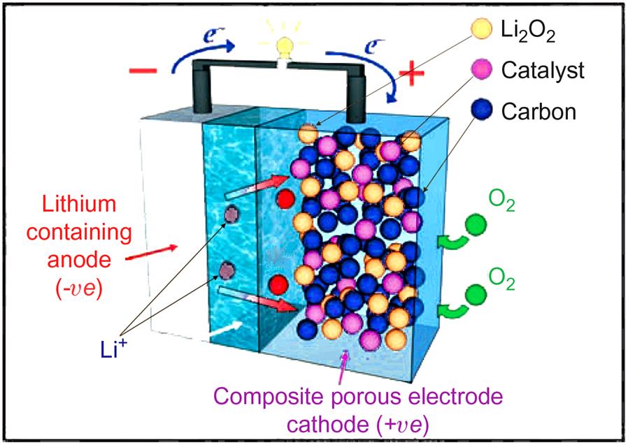
One solution to this problem is to copy the processes in green plants by having the reactants with a preference for recombination form on opposite sides of a membrane. The membranes could be formed using surface-active molecules. The artificial systems consist of a carbohydrate chain containing 5–20 atoms and, on one end, a molecule that associates easily with water (“hydrophilic group”). A double layer of such cells, with the hydrophilic groups facing in opposite directions, makes a membrane. If it is closed, for example, forming a shell (Fig. 5.27), it is called a micelle.
Consider now the photochemical reaction bringing A to an excited state A*, followed by ionization,
Under normal circumstances, the two ions would have a high probability of recombining, and the storage process would not be very efficient. But if A+ can be made to form in a negatively charged micelle, the expelled electron would react with B to form B− outside the micelle, and B− will not be able to react with A+. The hope is to be able to separate macroscopic quantities of the reactants, which would be equivalent to storing meaningful amounts of energy for later use (see, for example, Calvin, 1974), but efficiencies of artificial photosynthetic processes have remained low (Steinberg-Yfrach et al., 1998). Recently, matrix structures have been identified that delay the back-reaction by hours or more, but as yet the retrieval of the stored energy is made correspondingly more difficult. The materials are layered viologen compounds [such as N,N′-dimethyl-4,4′-bipyridinium chloride, methyl viologen (Slama-Schwok et al., 1992), or zirconium phosphate–viologen compounds with Cl and Br inserts (Vermeulen and Thompson, 1992)].
Research on photochemical storage of energy is at a very early stage and certainly not close to commercialization. If the research is successful, a new set of storage options will be available. However, it should be stressed that storage cycle efficiencies will not be very high. For photo-induced processes, the same limitations exist as for photovoltaic cells: for example, only part of the solar spectrum is useful and losses are associated with transitions through definite atomic and molecular energy states. Further losses are involved in transforming the stored chemicals to the energy form demanded.
5.5.12.3 Superconducting storage
A magnetic field represents energy stored. When a magnet is charged by a superconducting coil (e.g., a solenoid), heat losses in the coil may be practically zero, and the system constitutes an electromagnetic energy store with rapid access time for discharging. Maintenance of the coil materials (type II superconductors, such as NbTi) near the absolute zero temperature requires cryogenic refrigeration by, for example, liquid helium. Owing to the cost of structural support as well as protection against high magnetic flux densities around the plant, underground installation is envisaged. A storage level of 1 GJ is found in the scientific installation from the mid-1970s at the European physics laboratory CERN at Geneva (the installation aims at preserving magnetic energy across intervals between the accelerator experiments performed at the laboratory). A 100 GJ superconducting store has been constructed in the United States by the Department of Defense, who want to exploit the fact that superconducting stores can accumulate energy at modest rates but release it during very short times, as is required in certain antimissile defense concepts (Cultu, 1989). This is still a prototype development. Economic viability is believed to require storage ratings of 10–100 TJ, and, ideally, high-temperature superconductors can be used to reduce the cooling requirements (however, limited success has been achieved in raising the critical temperature; cf. Locquet et al., 1998).
Only type II superconductors are useful for energy storage purposes, since the superconducting property at a given temperature T (below the critical temperature that determines the transition between the normal and superconducting phase) disappears if the magnetic field exceeds a critical value, Bc(T) (magnetic field here is taken to mean magnetic flux density, a quantity that may be measured in units of tesla=V s m−2). Type II superconductors are characterized by a high Bc(T), in contrast to type I superconductors.
A magnetic field represents stored energy, with the energy density w related to the magnetic flux density (sometimes called magnetic induction) B by where μ0 (=1.26×10⁻⁶ henry m−1) is the vacuum permeability. When the superconducting coil is connected to a power source, the induced magnetic field represents a practically loss-free transfer of energy to the magnetic storage. With a suitable switch, the power source may be disconnected, and energy may later be retrieved by connecting the coil to a load circuit. Cycle efficiencies will not be 100%, owing to the energy required for refrigerating the storage. Since the magnetic field must be kept below the critical value Bc(T), increased capacity involves building larger magnets.
Conventional circuit components, such as capacitors, also represent an energy store, as do ordinary magnets. Such devices may be very useful to smooth out short-term variations in electrical energy flows from source to user, but they are unlikely to find practical uses as bulk storage devices.
Part II: Mini projects, discussion issues, and exercises
II.1
Find out what kinds of hourly and seasonal variations one can expect for the power production from a photovoltaic array mounted on an inclined rooftop in the area where you live.
You will need some solar radiation data for your local region. Satellite sources usually contain data only for horizontal surfaces, so it is better to find locally measured data for inclined surfaces suitable for solar panels. If such data are difficult to find, perhaps you can find separate solar radiation data for the direct and scattered parts (or for the direct and total radiation, from which you can derive the scattered radiation, at least if you assume it to be identical for any direction within a hemisphere). Such datasets are contained in reference-year data, which architects and consulting engineers use for design of buildings. Reference-year data exist for one or more urban locations in most countries of the world and allow you to calculate the total solar radiation falling on a particular inclined surface at a particular time of the day and the year. (Each particular time corresponds to a particular direction to the Sun, so that manipulating direct radiation becomes a simple geometric transformation. If you need help to calculate this relation, look in Chapter 3.).
You will also have to make assumptions on the function of the solar photovoltaic system. Initially, assume that it has a fixed efficiency for all sunlight. If you want to go further, you could include the wavelength-dependence of the panel efficiency, but, in that case, you need to know the frequency composition of the incoming radiation, which is more likely to be available from satellite data that may be found on the Internet.
II.2
Discuss the production of heat of the temperature TL from an amount of heat available, of temperature T above TL, and access to a large reservoir of temperature Tref below TL.
Quantities of heat with temperatures T and Tref may be simply mixed in order to obtain heat of the desired temperature.
Alternatively, a thermodynamic cycle may be used between the temperatures T and Tref to produce a certain amount of mechanical or electrical energy, which then is used to power the compressor of a heat pump, lifting heat from the Tref reservoir to the desired temperature TL.
As a variant, use a thermodynamic cycle between the temperatures T and TL, producing less work but on the other hand providing reject heat at the desired temperature. Again, a heat pump is used to provide more heat of temperature TL on the basis of the work output from the thermodynamic cycle.
What are the simple and the second law efficiencies in the individual cases?
II.3
Discuss design aspects of a propeller-type wind energy converter for which no possibility of changing the overall pitch angle θ0 is to be provided.
Consider, for instance, a design similar to the one underlying Figs. 4.17–4.22, but which is required to be self-starting at a wind speed of 2 m s−1 and to have its maximum power coefficient at a wind speed of 4 m s−1. Find the tip-speed ratio corresponding to this situation for a suitable overall pitch angle θ0 and for given assumptions on the internal torque Q0(Ω), e.g., that Q0 is independent of the angular velocity Ω, but proportional to the third power of the blade radius R, with the proportionality factor being given by
with ucut-in=2 m s−1.
Compare the power produced per square meter swept at a wind speed of 4, 6, and 10 m s−1 to the power that could be derived from a solar cell array of the same area.
For an actual design of wind energy converters, the blade shape and twist would not be given in advance, and one would, for a device with fixed angular velocity, first decide on this angular velocity (e.g., from generator and gearbox considerations) and then choose a design wind speed and optimize the blade shape c(r) and blade twist θ(r), in order to obtain a large power coefficient at the design speed and possibly to avoid a rapid decrease in the power coefficient away from the design point.
The blade shape c(r), of course, depends on blade number B, but to lowest order, the performance is independent of changes that leave the product of (cr) for the individual blades and B unchanged. Name some other considerations that could be important in deciding on the blade number.
II.4
In section 4.3.1, a maximum power coefficient Cp far above unity is suggested for certain cases of sail-driven propulsion on friction-free surfaces. Is this not a contradiction, like taking more power out than there is in the wind?
(Hint: Cp is defined relative to the wind power per unit area, which is of immediate relevance for rotors sweeping a fixed area. But what is the area seen by a sailing vessel moving with velocity U?).
II.5
Based, for example, on local data, such as those suggested in problem 1, what is the ratio between the daily amount of solar radiation that on a clear day in different seasons intercepts a fully tracking collector system, and the amount reaching a flat plate of fixed, south-facing orientation and a certain tilt angle s?
What is the relative importance of east–west tracking alone and solar height tracking alone?
II.6
Discuss shore-based wave energy converters, e.g., converters based on letting the wave trains ascend an inclined (and maybe narrowing) ramp, so that kinetic energy is converted into potential energy of elevation, which may be used to drive a turbine.
The simple solutions for gravity waves in a deep ocean, which were considered in the beginning of section 2.5.2, cannot be used directly for waves approaching shallow coastal waters. However, it may be assumed that the wave period remains unchanged, but that the amplitude a of the wave surface increases in such a way that the total power remains constant as the velocity potential becomes altered due to the boundary condition of no motion at the sea floor. This assumption implies the neglect of frictional dissipation at the sea floor.
There is a maximum ramp height that will permit a wave to reach the top and cross it into an elevated reservoir. If the turbine used requires a larger height to function well, a narrowing ramp construction may be used to give some fraction of the water mass the desired elevation.
II.7
Combine biomass productivity data with estimated efficiencies of fuel production by anaerobic fermentation processes (section 4.6.2) to give overall conversion efficiencies of bioconversion of solar energy into fuels. (A global biomass productivity map may be found in B. Sørensen: Biomass for energy: how much is sustainable? The map can be downloaded from the download-section at http://energy.ruc.dk; otherwise assume 1%–2% of incoming solar radiation converted into biomass.)
Compare this to other methods of converting solar radiation into mechanical or electrical work, and discuss their relative virtues other than conversion efficiency.
II.8
Estimate the magnitude of, and seasonal variation in, energy contained in stored food, separately for standing crops on the field, for livestock to be used for food, and for actually stored food (in grain stores, supermarkets, freezers, etc.). Compare food energy stored to the energy value of emergency stores of oil and natural gas, for example, in your own country.
(Hint: Data will have to be found at many different places. Some are in Chapter 6. You could estimate energy stored in supermarkets by your own spot checks of the declarations on typical food products, which should include their energy content.)
II.9
Estimate the potential world production of equivalent crude oil from Euphorbia plants, assuming only arid land is utilized and annual harvest yields are 40 MJ m−2. Areas of different types of land, including arid land, may be found on the Internet.
II.10
Consider a continuous-operation biogas digester for a one-family farm. The digester feedstock is pig slurry (collected daily) and straw (stored). The biogas is used for cooking, for hot water, and for space heating. Estimate the load curves for different seasons and calculate the volume of uncompressed gas storage required if load is to be met at any time during the year.
II.11
Consider pure methanol- and ethanol-driven cars, and, for comparison, a gasoline-driven car, weighing 800 kg and going on average 18 km per liter of gasoline and 500 km on a full tank. Calculate the mass penalties for methanol and ethanol fuel tanks, if the same operation range is required. Assume that the fuel usage varies linearly with total mass of the car.
II.12
Consider a thermal storage of temperature T (say, 200°C) aimed at receiving electric energy through a heat pump (with access to a reservoir of temperature Tref) and delivering electrical energy by means of a thermodynamic engine cycle (available coolant also of temperature Tref). What is the theoretical maximum cycle efficiency, and what can be expected in practice?
II.13
Discuss energy and power levels for the following “natural hydro energy” concept. Behind a seashore mountain chain there are a number of elevated water reservoirs (e.g., 200 m above sea level). The sea is characterized by a high evaporation rate (from solar energy), and the prevailing winds carry the evaporated water toward the coast, where a high percentage of the water returns to the land as rain on the mountainous region’s reservoirs (or imagine that precipitation is stimulated by seeding the clouds with some kind of condensation nuclei). Sample evaporation and precipitation rates may be found in meteorological tables or may be extracted from Chapter 2.
The water is returned from the reservoirs to the sea through hydropower plants. In a refined model, storage losses from the reservoirs due to evaporation should be included.
II.14
On the basis of time sequences of data for an automobile (e.g., your own), try to construct a load-duration curve for the entire period. Based on this, estimate a suitable level of rated power, if the engine should only cover average load, and specify the amount of storage needed for operating a hybrid car with a fuel-based engine rated at the average power needed, a battery store and an electric motor capable of delivering the maximum power required. The electric motor can be considered, to a good approximation, loss-free.
(Hint: A load-duration curve shows the fraction of time during which power demand exceeds a given value as a function of that power value.)
II.15
Construct the load-duration curve for space heating of a dwelling at your geographical location. Assume that this load is to be covered by an energy converter providing constant power all year and that loss-free heat storage is available. Determine the magnitude of the constant-converter output that, through use of storage, will suffice to cover the load at all times. Further, determine the minimum storage size needed. Compare the constant-converter output to the range of power provided by currently used heating systems. Use estimated losses for actual storage systems that may be relevant to assess what the required storage capacity would be in case the storage involved realistic losses.
II.16
A steam turbine power plant with a steam temperature of 700 K and a condenser temperature of 350 K has an efficiency of 0.36 (electric output energy divided by input steam energy), and the turbine efficiency is 20% less than the Carnot efficiency (εmax). Calculate the efficiency of the electric generator.
II.17
An electric vehicle of mass 1000 kg (excluding the battery) is designed for a 50 km range in a city driving cycle. The vehicle is equipped with a new 500 kg battery, and the average energy consumption is measured to be 0.3 kWh km−1 (from the battery). At a speed of 36 km h−1, the required acceleration is 2.0 m s−2, and the power required to overcome the frictional losses is one-third of the total power required. Do the same calculation for an acceleration a=1.5 m s−2.
II.18
Estimate the total hydro resource available for storage applications in a country or region. Characterize the natural reservoirs in terms of water volume and feasible turbine head, and identify the geological formations that could be considered for underground reservoir construction. In this way, arrive at rough storage capacities for short- and long-term storage separately. Estimation may be repeated for different regions and the results compared.
II.19
Use (5.39) to express the compressed storage energy (5.38) in terms of the temperature difference T−T0. rather than in terms of the pressure P.
II.20
Compare the energy needed to compress a certain amount of air by an adiabatic process with that required for an isothermal and an isobaric process.
II.21
Calculate the shape factor for a thin-rim flywheel, as well as mass- and volume-specific energy density, assuming the material to be steel. Do the same calculation numerically for some of the flywheel types shown in Fig. 5.18 (using data from Tables 5.6 and 5.7) and compare the properties. Discuss priorities for various types of application.