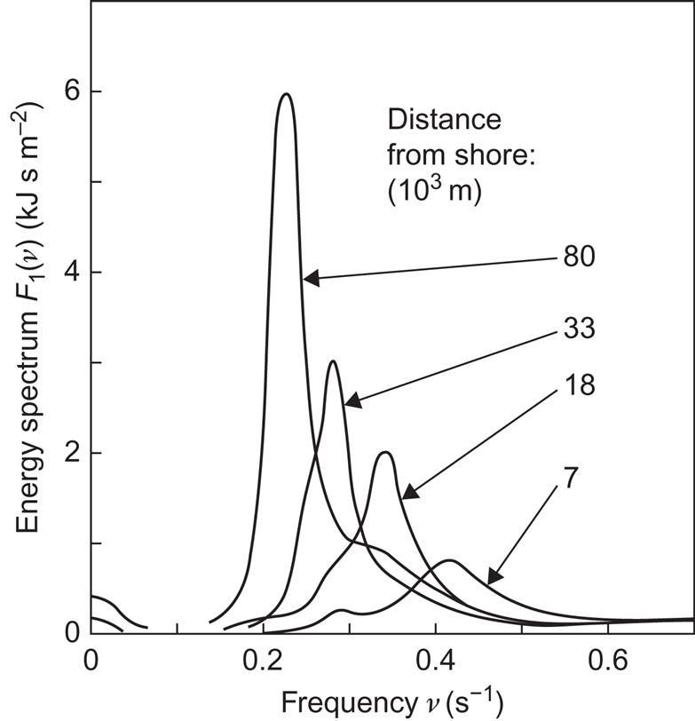
The position of the spectral peak will move downward as a function of time owing to non-linear wave–wave interactions, i.e., interactions between different spectral components of the wave field, as discussed in connection with (2.81) (Hasselmann, 1962). This behavior is clearly seen in the laboratory experiments of Mitsuyasu (1968), from which Fig. 3.53 shows an example of the time derivative of the energy spectrum, ∂F1(ν)/∂t. Energy is transferred from middle to smaller frequencies. In other experiments, some transfer is also taking place in the direction of larger frequencies. Such a transfer is barely present in Fig. 3.53. The shape of the rate-of-transfer curve is similar to the one found in later experiments for real oceanic conditions (Hasselmann et al., 1973), and both are in substantial agreement with the non-linear theory of Hasselmann.
Observations of ocean waves often exist in the form of statistics on the occurrences of given combinations of wave height and period. The wave height may be expressed as the significant height, Hs, or the root mean square displacement of the wave surface, Hrms. For a harmonic wave, these quantities are related to the surface amplitude, a, by
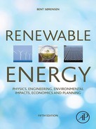
The period is usually given by the observed zero-crossing period. Figures 3.54 and 3.55 give examples of such measured frequency distributions, based on a year’s observation at the North Atlantic Station “India” (59°N, 19°W, the data quoted by Salter, 1974) and at the North Sea Station “Vyl” (55.5°N, 5.0°E, based on data discussed in Problem III.2). The probability of finding periods between 8 and 10 s and wave heights, a, between 0.3 and 1.5 m is quite substantial at Station India, of the order of 0.3. Also, the probability of being within a band of zero-crossing periods with a width of about 2 s and a center that moves slowly upward with increasing wave height is nearly unity (the odd values characterizing the contour lines of Fig. 3.54 are due to the original definition of sampling intervals in terms of feet and Hs).


3.3.4 Power in the waves
The power of a harmonic wave, i.e., the energy flux per unit length of wave crest, passing through a plane perpendicular to the direction of propagation, is from (2.84)
(3.28)
For the spectral distribution of energy given by the function F1 (section 3.3.1), each component must be multiplied by the group velocity ∂ω(k)/∂k. Taking ω=(gk)1/2 for ocean gravity waves, the group velocity becomes g/(2ω), and the power becomes
(3.29)
Based on observed energy spectra, F1, as a function of frequency or period T=2π/ω, the power distribution [(3.29) before integration] and total power may be constructed. Figure 3.56 gives the power distribution at the North Atlantic station also considered in Fig. 3.54. Using data for an extended period, the average distribution (labeled “year”) was calculated and, after extraction of data for the periods December–February and June–August, the curves labeled winter and summer were constructed (Mollison et al., 1976).

Compared with Fig. 3.34, for example, Fig. 3.56 shows that the seasonal variations in wave power at the open ocean site are substantial and equivalent to the seasonal variations in wind power at considerable height (maybe around 100 m, considering that the roughness length over the ocean is smaller than at the continental site considered in Fig. 3.36).
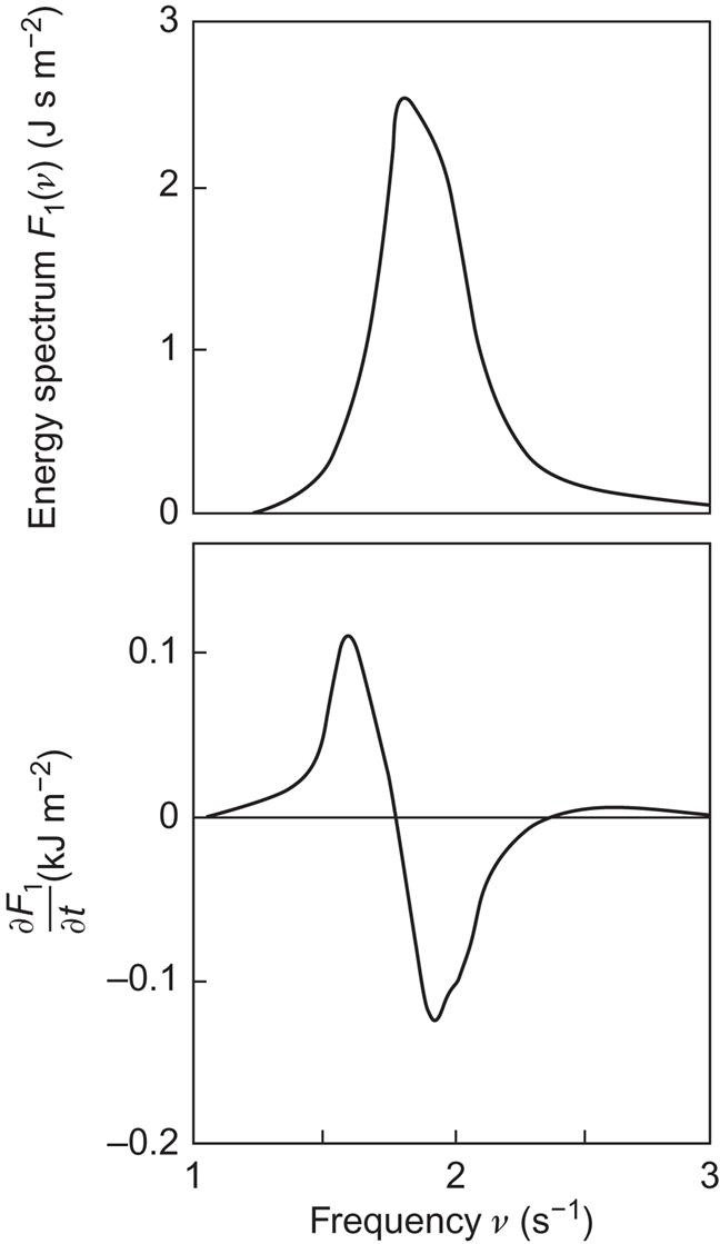
Figure 3.57 summarizes some of the data available on the geographical distribution of wave power. The figures given are yearly mean power at a specific location, and most of the sites chosen are fairly near to a coast, although still in open ocean. The proximity of a shore is important for energy extraction from wave motion. Whether such a condition will continue to apply will depend on the development of suitable methods for long-range energy transfer (Chapter 5).
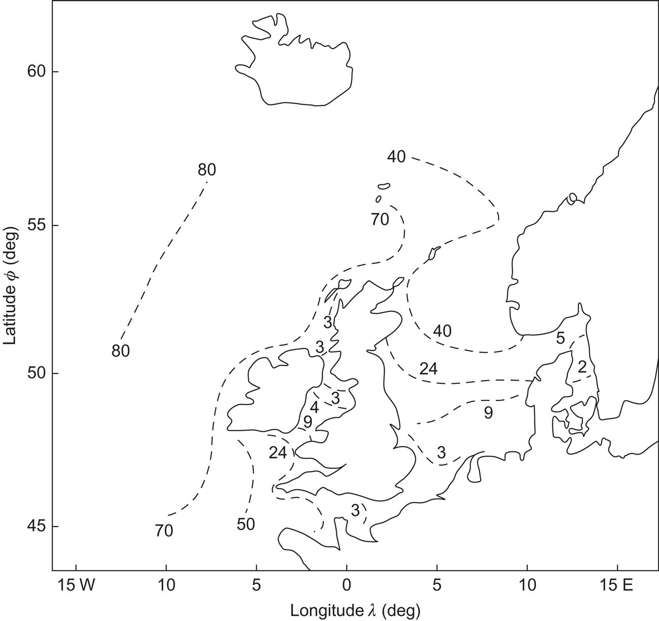
In Fig. 3.58, a more detailed map of wave power availability for the north European region is shown, based on the iso-power lines estimated in initial assessments of wave power in the United Kingdom, supplemented with estimates based on data for the waters surrounding Denmark. The rapid decrease in power after passing the Hebrides in approaching the Scottish coast from the Atlantic and also after moving southward through the North Sea is noteworthy.
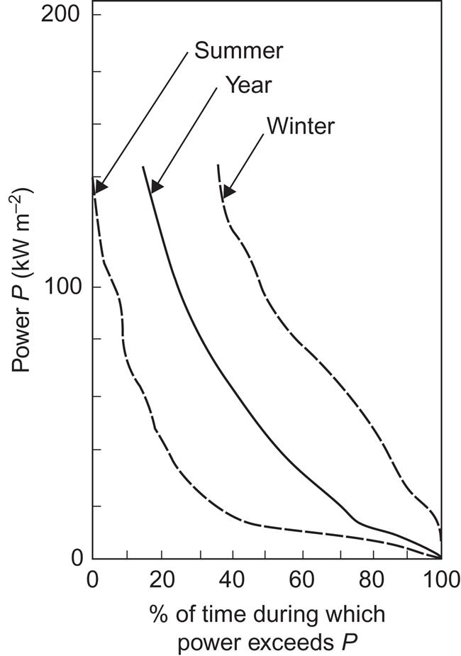
The variability of wave power may be described in terms similar to those used for wind energy. Figure 3.59 shows the power duration curves for Station India in the North Atlantic, based on all year or the summer or winter periods only, as in Fig. 3.56. Again, the occurrence of periods of low and high power depends markedly on seasonal changes.
3.3.4.1 Waves in a climatic context
As in the case of wind energy, little is known about the possible impact of large-scale energy extraction from wave power. One may argue that the total amount of energy involved is so small compared to the energy exchanged by atmospheric processes that any climatic consequence is unlikely. However, the exchange of latent and sensible heat, as well as matter, between the ocean and the atmosphere may, to a large extent, depend on the presence of waves. In particular, the rates of transfer may be high in the presence of breaking waves, and the extraction of energy from wave motion may prevent waves from developing a wave profile to the point of breaking. Thus, a study of the environmental implications of wave energy utilization, which seems to lend itself very naturally to computer simulation techniques, should be undertaken in connection with proposed energy extraction schemes. As suggested in previous sections, this is likely to be required for any large-scale use of renewable energy, despite the intuitive feeling that such energy sources are “non-polluting.” Yet the limited evidence available, mostly deriving from analogies to natural processes, does suggest that the results of more detailed analyses will be that renewable energy flows and stores can be utilized in quantities exceeding present technological capability, without worry about environmental or general climatic disturbances.
3.3.5 Tides
The average rate of dissipation of tidal energy, as estimated from the slowing down of the Earth’s rotation, is about 3×10¹² W. Of this, about a third can be accounted for by frictional losses in shallow sea regions, bays, and estuaries, according to Munk and MacDonald (1960).
In order to understand the concentration of tidal energy in certain coastal regions, a dynamic picture of water motion under the influence of tidal forces must be considered. The equations of motion for the oceans, (2.61) and (2.62), must be generalized to include the acceleration due to tidal attraction, that is, Ftidal/m where an approximate expression for the tidal force is given in (2.68). Numerical solutions to these equations (see, for example, Nihoul, 1977) show the existence of a complicated pattern of interfering tidal waves, exhibiting in some points zero amplitude (nodes) and in other regions deviations from the average water level far exceeding the “equilibrium tides” of a fraction of a meter (section 2.5.3). These features are in agreement with observed tides, an example of which is shown in Fig. 3.60. Newer data based on satellite measurements can be followed in near-real-time on the Internet (NASA, 2004).

The enhancement of tidal amplitudes in certain bays and inlets can be understood in terms of resonant waves. Approximating the inlet by a canal of constant depth h, the phase velocity of the tidal waves is Ut=(gh)1/2 (Wehausen and Laitone, 1960), and the wavelength is
where Tt is the period. For the most important tidal wave, Tt equals half a lunar day, and the condition for resonance may be written
(3.30)
where i is an integer, so that the length L of the inlet is a multiple of a quarter wavelength. For i=1, the resonance condition becomes L=34 973 h1/2 (L and h in meters). Bays and inlets satisfying this condition are likely to have high tidal ranges, with the range being the difference between highest and lowest water level. An example of this is the Severn inlet near Bristol in the United Kingdom, as seen from Fig. 3.60. Cavanagh et al. (1993) estimate the total European potential to be 54 GW or about 100 TWh y−1, of which 90% is in France and the United Kingdom.
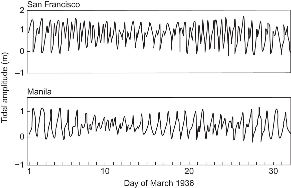
As discussed in section 2.5.3, the tides at a given location cannot be expected to have a simple periodicity, but rather are characterized by a superposition of components with different periods, the most important of which is equal to a half or full lunar or solar day. As a function of time, the relative phases of the different components change, leading to regularly changing amplitudes, of which two different patterns are shown in Fig. 3.61. The upper one is dominated by the half-day period, while the lower one is dominated by the full-day period.
If the water level at high tide, averaged over an area A, is raised by an amount H over the level at low tide, then the potential energy involved is
and the maximum power that could be extracted or dissipated would be, as an average over a tidal period Tt,
(3.31)
Based on measured tidal ranges, and on an estimate of the area A of a bay or inlet that could reasonably be enclosed by a barrage for the purpose of utilizing the energy flow (3.31), a number of favorable sites have been identified, as shown in Fig. 3.62. These include only localities with considerable concentration of tidal energy, because if the tidal range decreases, the area to be enclosed in order to obtain the same power increases quadratically, and the length of barrage will have to be correspondingly greater. For the same reason, sites of adequate tidal range, but no suitable bay, which could be enclosed by a reasonably small length of barrage, have been excluded. Of course, the term reasonable rests on an economic judgment that may be valid only under given circumstances. It is estimated that 2–3 GW may be extracted in Europe, half at costs in the range 10–20 euro-cents (or U.S. cents) per kWh (Cavanagh et al., 1993, using costing methodology of Baker, 1987), and 20–50 GW in North America (Sorensen and MacLennan, 1974; Bay of Fundy Tidal Power Review Board, 1977).

Environmental impacts may arise from utilization of tidal power. When the La Rance tidal plant was built in the 1960s, the upper estuary was drained for water over 2 years, a procedure that would hardly be considered environmentally acceptable today. Alternative building methods using caissons or diaphragms exist, but in all cases the construction times are long and careful measures have to be taken to protect the biosphere (e.g., when stirring up mud from the estuary seabed). Generally, the coastal environment is affected by the building and operation of tidal power plants, both during construction and to a lesser extent during operation, depending on the layout (fish bypasses, etc., as known from hydropower schemes). Some fish species may be killed in the turbines, and the interference with the periodic motion of bottom sand may lead to permanent siltation problems (and it has at La Rance).
The total estimated power of about 120 GW at the best sites throughout the world may be larger than what can be considered economical, but smaller than the amount of tidal energy actually available. It is still 12% of the above-mentioned estimate of the total dissipation of tidal energy in the vicinity of land, and it is unlikely that all the coastal sites yielding a total of 1000 GW would be suitable for utilization, so the order of magnitude is likely to be correct. The 2000 GW remaining [relative to the tidal power derived from astronomical data (Munk and MacDonald, 1960)] presumably becomes dissipated in the open ocean.
The maximal tidal power believed to be accessible, as well as the total resource estimate, is about 10% of the corresponding figures for hydropower, discussed in section 3.3.2. Tidal variations are coupled to river run-off and sea-level rise due to global greenhouse warming (Miller and Douglas, 2004).
3.4 Heat flows, reservoirs, and other sources of energy
A large fraction of incoming solar radiation is stored as heat near the surface of the Earth. According to Fig. 2.20, on average 47% is absorbed by the oceans and continents. The more detailed picture in Fig. 2.90 shows that 38% is absorbed by the oceans, 9% by the continents, and 24% by the atmosphere. Chapter 2 deals with some of the ways in which this energy could be distributed and eventually dissipated. Previous sections deal with the incoming radiation itself and with the kinetic energy in atmospheric and oceanic motion derived from the solar input by a number of physical processes. Storage of potential energy is also considered in connection with the processes of lifting water to a higher elevation, either in waves or in evaporated water, which may later condense and precipitate at a higher topographical level. Still, the energy involved in such kinetic and potential energy-creating processes is much less than the latent and sensible heat fluxes associated with the evaporation and condensation processes themselves and with the conversion of short-wavelength radiation to stored heat. The heat will be re-radiated as long-wavelength radiation in situations of equilibrium, but the temperature of the medium responsible for the absorption will rise, and in some cases the temperature gradients between the absorbing regions and other regions (deep soil, deep ocean, etc.), which do not themselves absorb solar radiation, cause significant heat flows.
Utilization of heat flows and stored heat may be direct if the desired temperature of use is no higher than that of the flow or storage. If this is not so, two reservoirs of different temperature may be used to establish a thermodynamic cycle yielding a certain amount of work, limited by the second law of thermodynamics. An alternative conversion scheme makes use of the heat pump principle by expending work added from the outside. Such conversion methods are considered in Chapter 4, while the focus here is on identifying the heat sources that are most suitable for utilization. The solar energy stores and flows are surveyed in section 3.4.1, whereas section 3.4.2 deals with the energy stored in the interior of the Earth and the corresponding geothermal flows.
3.4.1 Solar-derived heat sources
The ability of land and sea to act as a solar energy absorber and further as an energy store, to a degree determined by the local heat capacity and the processes that may carry heat away, is of profound importance for the entire biosphere. For example, food intake accounts only for 25%–30% of man’s total acquisition of energy during a summer day in central Europe (Budyko, 1974). The rest is provided by the body’s absorption of solar energy. The biological processes that characterize the present biosphere have vanishing rates if the temperature departs from a rather narrow range of about 270–320 K. Present forms of life thus depend on the greenhouse effect’s maintaining temperatures at the Earth’s surface in this range, at least during a fraction of the year (the growing season), and it is hard to imagine life on the frozen “white Earth” (see section 2.4.2) that would result if the absorption processes were minimized.
Utilization of heat stores and flows may then be defined as uses in addition to the benefits of the “natural” thermal regime of the Earth, but often no sharp division can be drawn between “natural” and “artificial” uses. For this reason, an assessment of the “magnitude” of the resource is somewhat arbitrary, and in each case it must be specified what is included in the resource base.
Total energy absorption rates are indicated in Fig. 2.90, and it is clear that the oceans are by far the most significant energy accumulators. The distributions of yearly average temperatures along cross-sections of the main oceans are shown in Figs. 2.67–2.69.
The potential of a given heat storage for heat pump usage depends on two temperatures: that of the storage and the required usage temperature. This implies that no energy “amount” can be associated with the energy source, and a discussion of heat pump energy conversion is therefore deferred to Chapter 4. An indication of possible storage temperatures may be derived from Figs. 2.67–2.69 for the oceans, Fig. 2.103 for a continental site, and Fig. 2.32 for the atmosphere.
For utilization without addition of high-grade mechanical or electric energy, two reservoirs of differing temperatures must be identified. In the oceans, Figs. 2.67–2.69 indicate the presence of a number of temperature gradients, most noticeable at latitudes below 50° and depths below 1000–2000 m. Near the Equator, the temperature gradients are largest over the first few hundred meters, and they are seasonally stable, in contrast to the gradients in regions away from the Equator, which are largest during summer and approach zero during winter. At still higher latitudes, there may be ice cover during a part or all of the year. The temperature at the lower boundary of the ice, i.e., at the water–ice interface, is almost constantly equal to 271.2 K (the freezing point of seawater), and in this case a stable temperature difference can be expected between the water and the atmosphere, particularly during winter.
It follows from Fig. 2.90 that over half the solar energy absorbed by the oceans is used to evaporate water. Of the remaining part, some will be transferred to the atmosphere as sensible heat convection, but most will eventually be re-radiated to the atmosphere (and maybe to space) as long-wavelength radiation. The length of time during which the absorbed energy will stay in the oceans before being used in one of the above ways, determines the temperature regimes. At the ocean surface, residence times of a fraction of a day are associated with diurnal temperature variations, while residence times normally increase with depth and reach values of several hundred years in the deepest regions (section 2.3.2).
If oceanic temperature gradients are used to extract energy from the surface region, a cooling of this region may result, unless the currents in the region are such that the cooling primarily takes place elsewhere. A prediction of the climatic impact of heat extraction from the oceans thus demands a dynamic investigation like the one offered by the general circulation models discussed in section 2.3.2. The energy extraction would be simulated by an additional source term in (2.65), and attention should be paid to the energy loss from the ocean’s surface by evaporation, which would decrease at the places with lowered temperatures. Extraction of energy from the oceans may for this reason lead to an increase of the total downward energy flux through the surface, as noted by Zener (1973). In addition to possible climatic effects, oceanic energy extraction may have an ecological effect, partly because of the temperature change and partly because of other changes introduced by the mixing processes associated with at least some energy conversion schemes (e.g., changing the distribution of nutrients in the water). Assuming a slight downward increase in the concentration of carbon compounds in seawater, it has also been suggested that artificial upwelling of deep seawater (used as cooling water in some of the conversion schemes discussed in Chapter 4) could increase the CO2 transfer from ocean to atmosphere (Williams, 1975).
3.4.1.1 The power in ocean thermal gradients
In order to isolate the important parameters for assessing the potential for oceanic heat conversion, Fig. 3.63 gives a closer view of the temperature gradients in a number of cases with large and stable gradients. For locations at the Equator, seasonal changes are minute, owing to the small variations in solar input. For locations in the Florida Strait, the profiles are stable, except for the upper 50–100 m, owing to the Gulf Stream transport of warm water originating in tropical regions. The heat energy content relative to some reference point of temperature Tref is cV(T – Tref), but only a fraction of this can be converted to mechanical work, and the direct use of water at temperatures of about 25°C above ambient is limited, at least in the region near the Equator. Therefore, in aiming at production of mechanical work or electricity, the heat value must be multiplied by the thermodynamic efficiency (cf. Chapter 4), i.e., the maximum fraction of the heat at temperature T that can be converted to work. This efficiency, which would be obtained by a hypothetical conversion device operating in accordance with an ideal Carnot cycle, is (cf. section 4.1.2)
(3.32)
where the temperatures should be in K.

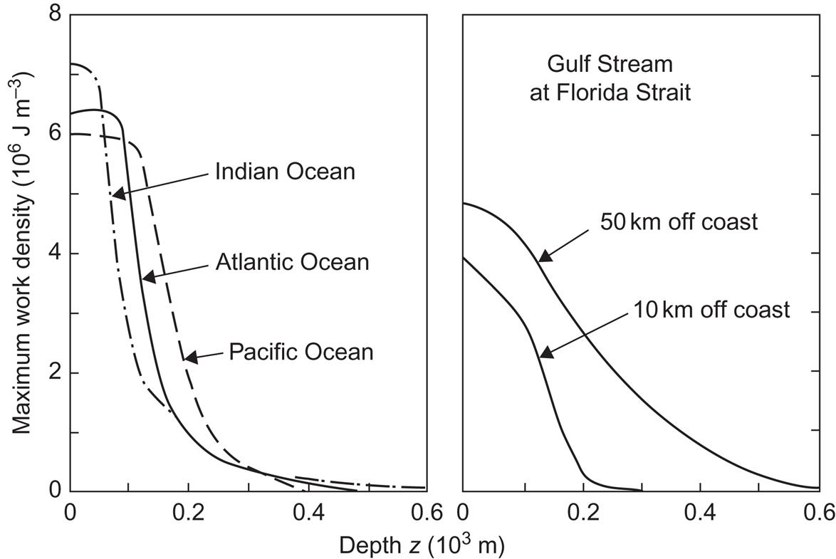
Taking the reference temperature (the “cold side”) as Tref=6°C, corresponding to depths of 380 m (Gulf Stream, 10 km from coast), 680 m (Gulf Stream, 50 km from coast), 660 m (Atlantic Ocean), 630 m (Pacific Ocean), and 1000 m (Indian Ocean) (see Fig. 3.63), one obtains the maximum energy that can be extracted from each cubic meter of water at temperature T (as a function of depth), in the form of mechanical work or electricity,
This quantity is shown in Fig. 3.64 for the sites considered in the preceding figure. It is seen that, owing to quadratic dependence on the temperature difference, the work density is high only for the upper 100 m of the tropical oceans. Near the coast of Florida, the work density drops more slowly with depth, owing to the presence of the core of the warm Gulf Stream current (cf. Fig. 3.50). Below the current, the work density drops with a different slope, or rather different slopes, because of the rather complex pattern of weaker currents and countercurrents of different temperatures.
The power that could be extracted is obtained by multiplying the work density by the transfer coefficient of the conversion device, that is, the volume of water from which a maximum energy prescribed by the Carnot value can be extracted per second. This quantity is also a function of T and Tref, and losses relative to the ideal Carnot process are included in terms of a larger “effective” volume necessary for extracting a given amount of work. If the device were an ideal Carnot machine and the amount of water processed were determined by the natural flow through the device, then at a flow rate of 1 m s−1 (typical of the Gulf Stream current) the power extracted would be 3–4 MW m−2 facing the current flow direction, according to Fig. 3.64. In practice, as the treatment in Chapter 4 shows, only a fraction of this power will be obtained.
An indication of the global distribution of locations with large ocean temperature gradients may be obtained from Fig. 3.65, which gives the average temperature difference between the surface water and the water at a depth of 200 m for the time of the year when this difference is smallest. As mentioned above, seasonal variation is very small in the equatorial region, whereas the summer temperature difference is far greater than the winter temperature difference at mid- and high latitudes, as seen from Fig. 3.66.
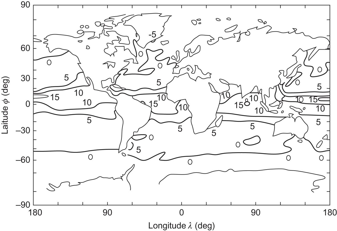

The availability of currents that could promote flow through a temperature-gradient-utilizing device may be estimated from the material in section 3.3.1, but it should be borne in mind that the currents are warm only after passage through the equatorial region. It then follows from Fig. 3.42 that most currents on the Northern Hemisphere are warm, while most currents in the Southern Hemisphere originate in the Antarctic region and are cold.
3.4.1.2 Temperature gradients in upper soil and air
The temperature gradient due to absorption of solar radiation in continental soil or rock has a diurnal and a seasonal component, as discussed in section 2.3.2. Transport processes in soil or rock are primarily by conduction rather than by mass motion (ground water does move a little, but its speeds are negligible compared with ocean currents), which implies that the regions that are heated are much smaller (typically depths of up to 0–7 m in the diurnal cycle and up to 15 m in the seasonal cycle). The seasonal cycle may be practically absent for locations in the neighborhood of the Equator. An example of the yearly variation at fairly high latitude is given in Fig. 2.103. The picture of the diurnal cycle is very similar except for scale, as follows from the simple model given by (2.40)–(2.42). Therefore, the potential for extracting mechanical work or electricity from solar-derived soil or rock temperature gradients is very small. Direct use of the heat is usually excluded as well, because the temperatures in soil or rock are mostly similar to or slightly lower than that of the air. An exception may be dry rock, which can reach temperatures substantially above the ambient after some hours of strong solar exposure. Extraction of heat from soil or rock by means of the heat pump principle is possible and is discussed in the next chapter.
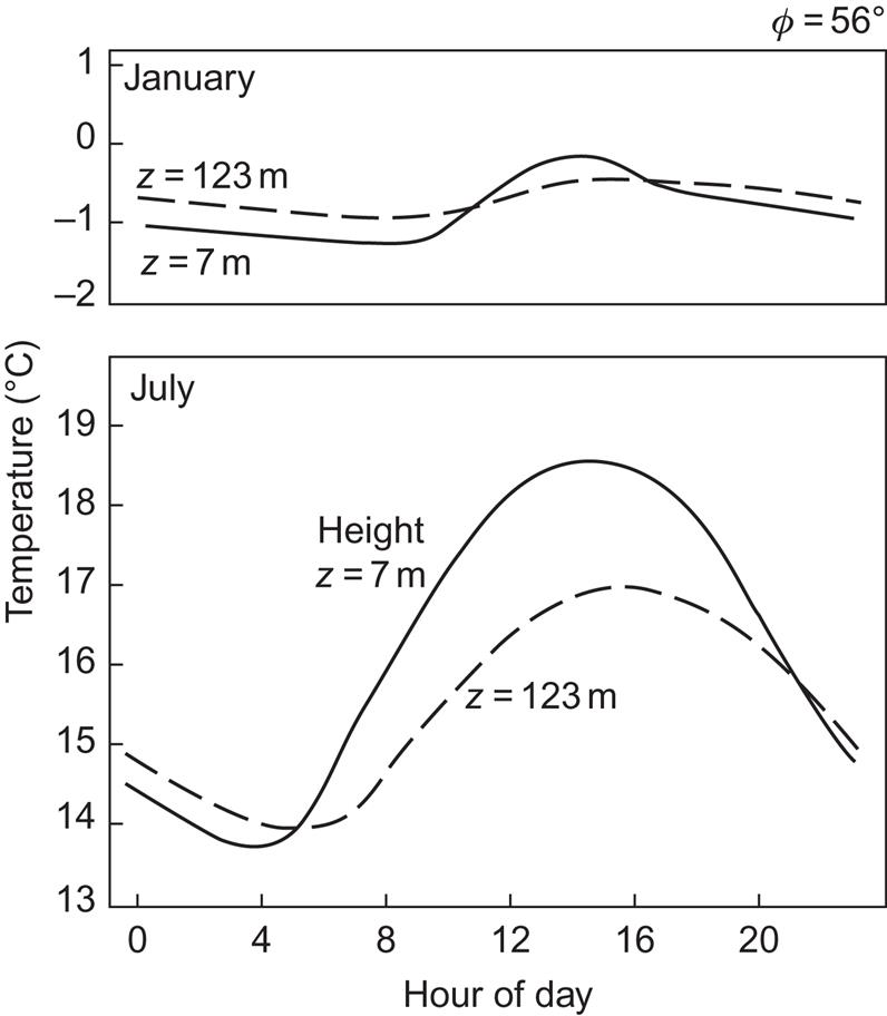
Temperature gradients in the atmosphere are rather small but of stable sign (except for the layer near the ground) up until the tropopause (see Fig. 2.29). At higher altitudes, the gradient changes sign a few times (Fig. 2.28). The temperature gradient over the first few hundred meters above ground is largely determined by the sign of the net total radiation flux, which exhibits a daily cycle (cf. Fig. 2.1) characterized by downward net flux during daylight and upward net flux at night. An example of the corresponding diurnal variation in temperature at heights of 7 and 123 m is shown in Fig. 3.67 for January and July at a location 56°N.
The density of air also decreases with height (Fig. 2.28), and the heat capacity is small (e.g., compared with that of water), so the potential for energy conversion based on atmospheric heat is small per unit of volume. Energy production using the atmospheric temperature gradient would require the passage of very large quantities of air through an energy extraction device, and the cold air inlet would have to be placed at an elevation kilometers above the warm air inlet. However, heat pump use of air near ground level is possible, just as it is for solar energy stored in the upper soil.
3.4.2 Geothermal flows and stored energy
Heat is created in some parts of the interior of the Earth: as a result of radioactive disintegration of atomic nuclei. In addition, the material of the Earth is in the process of cooling down from an initial high temperature or as a result of heat carried away after being released within the interior by condensation and possibly other physical and chemical processes.
3.4.2.1 Regions of particularly high heat flow
Superimposed on a smoothly varying heat flow from the interior of the Earth toward the surface are several abnormal flow regions. The subsurface temperature exhibits variations associated with the magnitude of the heat flow and heat capacity—or, in general, the thermal properties—of the material. The presence of water (or steam) and other molten material is important for the transportation and concentration of heat. Until now, the vapor-dominated concentrations of geothermal energy have attracted the most attention as potential energy extraction sources. However, the occurrence of hot springs or underground steam reservoirs is limited to a very few locations. Reservoirs containing superheated water (brine) are probably more common, but are hard to detect from general geological data.
Some reservoirs attract special interest owing to chemical processes in brine–methane mixtures that release heat and increase the pressure, while the conductivity of such mixtures is low (so-called geo-pressurized systems, cf. Rowley, 1977). Dry rock accumulation of heat is probably the most common type of geothermal heat reservoir (i.e., storage with temperature above average), but it does not lend itself so directly to utilization because of the difficulties in establishing sufficiently large heat transfer surfaces. A number of high-temperature reservoirs are present in volcanic systems in the form of lava pools and magma chambers.
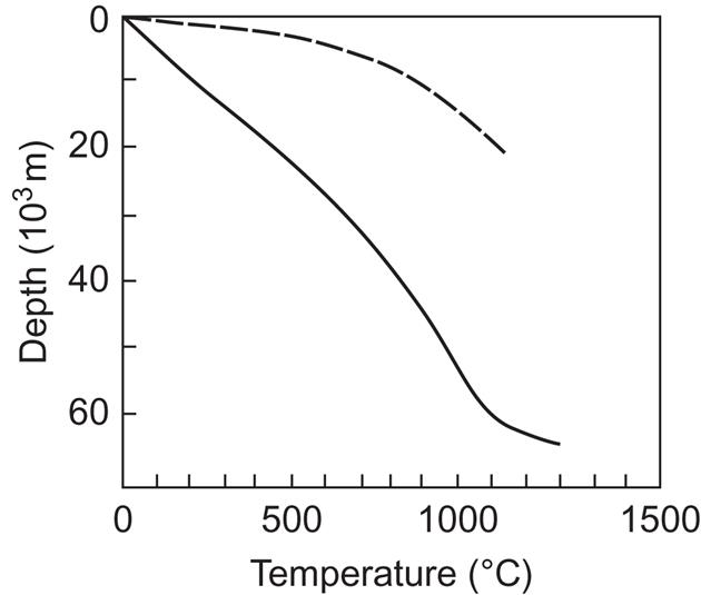
Whereas the smoothly varying average heat flow from the interior of the Earth can be considered a renewable energy resource (see below), the reservoirs of abnormal temperature are not necessarily large in relation to possible usage and do not get renewed at rates comparable to possible extraction rates. It is estimated that electric power generation by use of geothermal steam at the locations where such steam is available will be possible for only about 50 years. The total amount of geothermal heat stored in water or steam to a depth of 10 000 m is estimated to be 4×10²¹ J, of which some (1–2)×1020 J is capable of generating steam of above 200°C (World Energy Conference, 1974). The same source estimates the total amount of energy stored in dry rocks to a depth of 10 km as around 1027 J. Steam of temperatures above 200°C represents an average power of 240×109 W for a period of 50 years.
It follows from the above that most of the abnormal geothermal heat reservoirs must be considered non-renewable resources on the same footing as fossil and fissile deposits. However, the average geothermal heat flow also corresponds to temperature gradients between the surface and reachable interior of the Earth, which can be used for energy extraction, at least if suitable transfer mechanisms can be established. These may be associated with water flow in regions of high permeability, so that water that has been cooled by an energy extraction device may regain the temperature of the surrounding layer in a relatively short time.
3.4.2.2 The origin of geothermal heat
The radioactive elements mainly responsible for geothermal heat production at present are 235U (decay rate 9.7×10⁻¹⁰ year−1), 238U (decay rate 1.5×10⁻¹⁰ year−1), 232Th (decay rate 5.0×10⁻¹¹ year−1), and 40K (decay rate 5.3×10⁻¹⁰ year−1). These isotopes are present in different concentrations in different geological formations. They are more abundant in the granite-containing continental shields than in the ocean floors. Most of the material containing the radioactive elements is concentrated in the upper part of the Earth’s crust. In the lower half of the crust (total depth around 40 km), radiogenic heat production is believed to be fairly constant, at a value of about 2×10⁻⁷ W m−3 (Pollack and Chapman, 1977). The rate of radiogenic heat production at the top of the continental crust is typically at least ten times higher, but it decreases with depth and reaches the lower crust value approximately halfway through the crust. The amount of radioactivity in the mantle (occupying the volume between the core and the crust) and in the core (the radius of which is about half the total radius) is poorly known, but models indicate that very little radioactive heat production takes place in the mantle or core.
From the radioactive decay of the above-mentioned isotopes, it can be deduced that the temperature of an average piece of rock near the surface of the crust must have decreased some 900°C during the last 4.5×10⁹ years (i.e., since the Sun entered the main burning sequence; Goguel, 1976). At present, radiogenic heat production accounts for an estimated 40% of the continental average heat flow at the surface. The rest, as well as most of the heat flow at the oceanic bottom, may then be due to cooling associated with expenditure of stored heat.
In order to assess the nature and origin of the heat stored in the interior of the Earth, the creation and evolution of the planet must be modeled. As discussed in section 2.1.1, the presence of heavy elements in the Earth’s crust would be explained if the material forming the crust was originally produced during one or more supernovae outbursts. It is also consistent to assume that this material was formed over a prolonged period, with the last contribution occurring some 108 years before the condensation of the material forming the Earth (Schramm, 1974).
A plausible model of the formation of the planetary system assumes an initial nebula of dust and gases (including the supernova-produced heavy elements), the temperature of which would increase toward the center. The Sun might then be formed by gravitational collapse (cf. section 2.1.1). The matter not incorporated into the “protosun” would slowly cool, and parts of it would condense into definite chemical compounds. The planets would be formed by gravitational accretion of matter, at about the same time as, or slightly earlier than, the formation of the Sun (Reeves, 1975).
One hypothesis is that the temperature at a given distance from the protosun would be constant during the formation of planets like the Earth (equilibrium condensation model; see, for example, Lewis, 1974). As temperature declines, a sequence of condensation processes occurs: at 1600 K, oxides of calcium, aluminum, etc.; at 1300 K, nickel–iron alloys; at 1200 K, enstatite (MgSiO3); at 1000 K, alkali-metal-containing minerals (feldspar, etc.); at 680 K, troilite (FeS). The remaining iron would be progressively oxidized, and, at about 275 K, water would be formed. The assumption that the Earth was formed at a constant temperature of about 600 K implies that it would have a composition characteristic of the condensation state at that temperature.
Other models can be formulated that would also be relatively consistent with the knowledge of the (initial) composition of the Earth’s interior. If, for example, the planet formation process was slow compared to the cooling of the nebula, then different layers of the planet would have compositions characteristic of different temperatures and different stages of condensation.
It is also possible that the creation of the Sun and the organization of the primordial nebula did not follow the scheme outlined above, but were the results of more violent events, such as the close passage of a supernova star.
If the assumption of a constant temperature of about 600 K during the formation of the Earth is accepted, then the subsequent differentiation into crust, mantle, and core (each of the latter two having two subdivisions) is a matter of gravitational settling, provided that the interior was initially in the fluid phase or that it became molten as a result of the decay of radioactive isotopes (which, as mentioned, must have been much more abundant at that time, partly because of the exponential decay of the isotopes present today and partly owing to now-absent short-lived isotopes). The crust would have formed very quickly as a result of radiational cooling, but the presence of the crust would then have strongly suppressed further heat loss from the interior. The central region may have been colder than the mantle during the period of core formation by gravitational settling (Vollmer, 1977).
Gravitational settling itself is a process by which gravitational (potential) energy is transformed into other energy forms. It is believed that most of this energy emerged as heat, and only a smaller fraction as chemical energy or elastic energy. If the differentiation process took place over a short time interval, the release of 26×1030 J would have heated material of heat capacity similar to that of crustal rocks to a temperature of about 5000 K. If the differentiation was a prolonged process, then the accompanying heat would, to a substantial extent, have been radiated into space, and the temperature would never have been very high (Goguel, 1976). The present temperature increases from about 300 K at the surface to perhaps 4000 K in the center of the core. During the past, convective processes as well as formation of steam plumes in the mantle are likely to have been more intense than at present. The present heat flow between the mantle and the crust is about 25×1012 W, while the heat flow at the surface of the crust is about 30×1012 W (Chapman and Pollack, 1975; Pollack and Chapman, 1977).
If heat conduction and convective processes of all scales can be approximately described by the diffusion equation (2.28), supplemented with a heat source term describing the radioactive decay processes, in analogy to the general transport equation (2.44), then the equation describing the cooling of the Earth may be written
(3.33)
where K is the effective diffusion coefficient and S is the radiogenic heat production divided by the local heat capacity C. The rate of heat flow is given by
(3.34)
where the thermal conductivity λ equals KC, according to (2.39). If the temperature distribution depends only on the radial co-ordinate r, and K is regarded as a constant, (3.33) reduces to
(3.35)
The simplified version is likely to be useful only for limited regions. The diffusion coefficient K is on average of the order of 10−6 m2 s−1 in the crust and mantle, but increases in regions allowing transfer by convection. The thermal conductivity λ of a material depends on temperature and pressure. It averages about 3 W m−1 K−1 in crust and mantle, but may be much higher in the metallic regions of the core. The total amount of heat stored in the Earth (relative to the average surface temperature) may be estimated from ∫volumeλK−1(T – Ts)dx, which has been evaluated as 4×1030 J (World Energy Conference, 1974). Using the average heat outflow of 3×10¹³ W, the relative loss of stored energy presently amounts to 2.4×10⁻¹⁰ per year. This is the basis for treating the geothermal heat flow on the same footing as the truly renewable energy resources. Also, in the case of solar energy, the energy flow will not remain unchanged for periods of the order billions of years, but will slowly increase, as discussed in sections 2.1.1 and 2.4.2, until the Sun leaves the main sequence of stars (at which time the radiation will increase dramatically).
3.4.2.3 Distribution of the smoothly varying part of the heat flow
The important quantities for evaluating the potential of a given region for utilization of the geothermal heat flow are the magnitude of the flow and its accessibility.
The temperature gradient and heat flow are usually large in young geological formations and, in particular, at the mid-oceanic ridges, which serve as spreading centers for the mass motion associated with continental drift. In the continental shields, the gradient and flow are much smaller, as illustrated in Fig. 3.68. Along sections from the mid-oceanic ridges to the continental shields, the gradient may gradually change from one to the other of the two types depicted in Fig. 3.68. In some regions the temperature gradients change much more abruptly (e.g., in going from the Fenno-Scandian Shield in Norway to the Danish Embayment; cf. Balling, 1976), implying in some cases a high heat flux for land areas (e.g., northwestern Mexico, cf. Smith, 1974).
Maps of the geographical distribution of heat flow, both at the surface of the crust and at the surface of the mantle, have been prepared by Chapman and Pollack (1975; Pollack and Chapman, 1977) by supplementing available data with estimates based on tectonic settling and, for oceanic regions, the age of the ocean floor. The results, shown in Figs. 3.69a and b, are contours of a representation in terms of spherical harmonic functions of latitude and longitude, Ylm(ϕ, λ), of maximum degree l=12. The advantage of this type of analysis is that oscillations of wavelength smaller than about 3000 km will be suppressed, so that the maps are presumably describing the smoothly varying average flow without perturbations from abnormal flow regions. A comparison between the calculation shown in Fig. 3.69a and one in which the model predictions have also been used in regions where measurements do exist, has convinced Chapman and Pollack that little change will result from future improvements in the data coverage. The map showing the mantle flow, Fig. 3.69b, is obtained by subtracting the contribution from the radiogenic heat production in the crust from the surface flow map. To do this, Pollack and Chapman have used a model for the continental regions in which the heat production decreases exponentially from its local value at the surface of the crust,
where b=8.5 km (if not measured), until it reaches the constant value CS=2.1×10⁻⁷ W m−3 assumed to prevail throughout the lower crust. For oceanic regions, the difference between mantle and surface heat flows is estimated on the basis of the cooling of the oceanic crust (assumed to behave like a 6.5-km thick layer of basalt) with a fixed lower boundary temperature of 1200°C. The time during which such cooling has taken place (the “age” of the sea floor) is determined from the present surface heat flow (Pollack and Chapman, 1977).
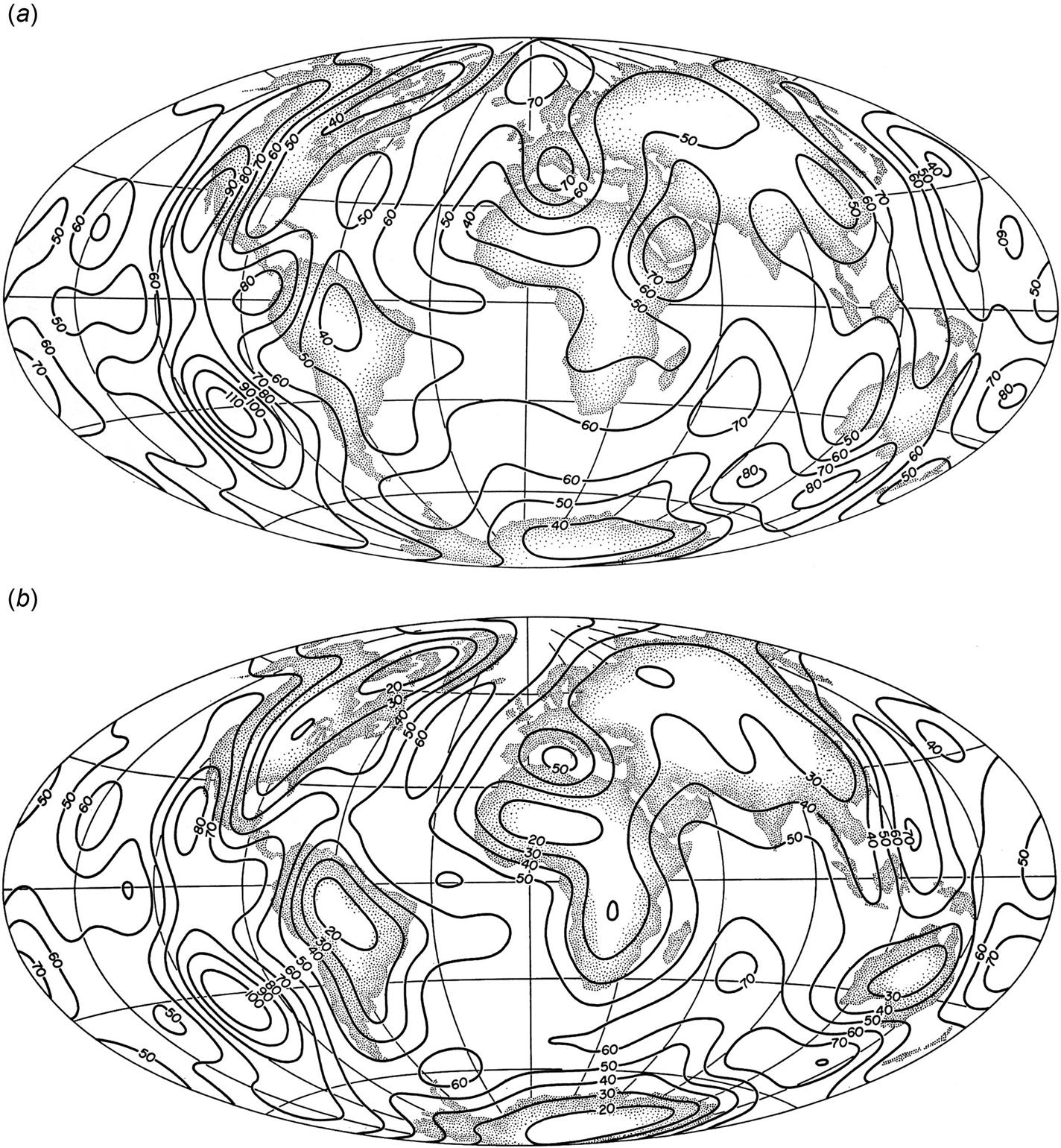
Mantle heat flow is very regular, with low continental values and increasing flow when approaching the oceanic ridges, particularly in the southern Pacific Ocean. The surface heat flow is considerably more irregular, in a manner determined by the composition of the crust at a given location, but the mean fluctuation around the average value of 5.9×10⁻² W m−2 is only 22%. The surface heat flow has similar values if evaluated separately for continents and oceans (5.3 and 6.2×10⁻² W m−2, respectively), while the contrast is larger for the upper mantle flow (2.8 and 5.7×10⁻² W m−2, respectively).
The usefulness of a given flow for purposes of energy extraction depends on the possibilities for establishing a heat transfer zone of sufficient flux. As mentioned earlier, the most appealing heat transfer method is by circulating water. In this case, the rate of extraction depends on the permeability of the geological material (defined as the fluid speed through the material, for a specified pressure gradient and fluid viscosity). The pressure is also of importance in determining whether hot water produced at a depth will rise to the top of a drill-hole unaided, or will have to be pumped to the surface. High permeability is likely to be found in sand-containing sedimentary deposits, while granite and gneiss rock have very low porosity and permeability. Schemes for hydraulic fractionation or granulation caused by detonation of explosives have been proposed, with the purpose of establishing a heat transfer area large enough that vast areas of hot rock formations could be accessed for extraction of geothermal energy, for example, by circulating water through man-made regions of porous material.
3.4.3 Ocean thermal and salinity gradients
The preceding parts of this chapter are concerned with renewable energy flows and stores based on solar radiation, gravitation between celestial bodies, the mechanical energy involved in atmospheric and oceanic circulation, as well as a number of (sensible or latent) heat sources, the origin of which were solar or geological. It is believed that the most important of such sources are listed, but some significant sources may have been omitted.
In the description of heat sources, in particular, the list is far from complete, considering that any difference in temperature constitutes a potential source of energy. It may not be practical to attempt to extract energy from the difference in air or soil temperature between the Arctic and Equatorial regions, but the corresponding difference in water temperature is, in fact, the basis for the temperature gradients in some oceanic regions (discussed in section 3.4.2), owing to water transport by currents. One case in which a stable temperature difference might be usable in ways similar to those proposed for ocean temperature gradients is offered by the difference between the Arctic air temperature and the water temperature at the base of the ice sheets covering Arctic oceans. The average air temperature is about –25°C for the period October–March, but the temperature at the ice–water interface is necessarily close to 0°C (although not quite zero because of salinity- and pressure-induced depreciation of the freezing point, cf. Fig. 3.66). Other ocean thermal energy conversion (OTEC) proposals have focused on the temperature difference between warm currents, such as the Gulf Stream, and surrounding, colder bodies of water. The temperature difference is small and a thermodynamic engine working between such temperatures will have exceedingly low efficiency. In addition, tampering with currents like the Gulf Stream could have large environmental effects on the regions depending on heat delivery from warm currents (such as Northern Europe in the case of the Gulf Stream).
It is natural to ask whether other energy forms, such as electromagnetic, earthquake, chemical (of which bioenergy is treated in section 3.5), or nuclear energy, can be considered as energy resources and to what extent they are renewable. Examples of such energy forms are discussed in sections 3.4.4 and 3.4.5.
Useful chemical energy may be defined as energy that can be released through exothermic chemical reactions. In general, chemical energy is associated with chemical bonds between electrons, atoms, and molecules. The bonds may involve overlapping electron wavefunctions of two or more atoms, attraction between ionized atoms or molecules, and long-range electromagnetic fields created by the motion of charged particles (notably electrons). In all cases, the physical interaction involved is the Coulomb force. Examples of chemical energy connected with molecular bonds are given in section 3.5 (bioenergy sources, including fossil fuels).
The organization of atoms or molecules in regular lattice structures represents another manifestation of chemical bonds. Some substances possess different crystalline forms that may exist under given external conditions. In addition to the possibility of different solid phases, phase changes associated with transitions among solid, liquid, and gas phases all represent different levels of latent energy.
3.4.3.1 Salinity differences
Solutions represent another form of chemical energy, relative to the pure solvent. The free energy of a substance with components i=1, 2, …, there being ni mol of the ith component, may be written
(3.36)
where μi is the chemical potential of component i. For a solution, μi can be expressed in the form (see, for example, Maron and Prutton, 1959)
(3.37)
where ![]() is the gas constant (8.3 J K−1 mol−1), T is the temperature (K), and xi=ni/(Σjnj) the mole fraction.
is the gas constant (8.3 J K−1 mol−1), T is the temperature (K), and xi=ni/(Σjnj) the mole fraction. ![]() is the chemical potential that would correspond to xi=1 at the given pressure P and temperature T, and fi is the activity coefficient, an empirical constant that approaches unity for ideal solutions, an example of which is the solvent of a very dilute solution (whereas, in general, fi cannot be expected to approach unity for the dissolved component of a dilute solution).
is the chemical potential that would correspond to xi=1 at the given pressure P and temperature T, and fi is the activity coefficient, an empirical constant that approaches unity for ideal solutions, an example of which is the solvent of a very dilute solution (whereas, in general, fi cannot be expected to approach unity for the dissolved component of a dilute solution).
It follows from (3.36) and (3.37) that a solution represents a lower chemical energy than the pure solvent. The most common solution present in large amounts on the Earth is saline ocean water. Relative to this, pure or fresh water, such as river run-off, represents an elevated energy level. In addition, there are salinity differences within the oceans, as shown in Figs. 2.67–2.69.
Taking the average ocean salinity as about 33×10−3 (mass fraction), and regarding this entirely as ionized NaCl, nNa+=nCl− becomes about 0.56×10³ mol and nwater=53.7×10³ mol, considering a volume of 1 m3. The chemical potential of ocean water, μ, relative to that of fresh water, μ0, is then from (3.37)
Consider now a membrane that is permeable for pure water but impermeable for salt (i.e., for Na+ and Cl− ions) as indicated in Fig. 3.70. On one side of the membrane, there is pure (fresh) water, on the other side saline (ocean) water. Fresh water will flow through the membrane, trying to equalize the chemical potentials μ0 and μ initially prevailing on each side. If the ocean can be considered as infinite and being rapidly mixed, then nNa+ will remain fixed, also in the vicinity of the membrane. In this case each m3 of fresh water penetrating the membrane and becoming mixed will release an amount of energy, which from (3.49) is
(3.38)

For a temperature T≈285 K (considered fixed), δG≈2.65×10⁶ J. The power corresponding to a fresh-water flow of 1 m3 s−1 is thus 2.65×10⁶ W (cf. Norman, 1974). The worldwide run-off of about 4×10¹³ m3 y−1 (Fig. 2.65) would thus correspond to an average power of around 3×10¹² W.
The arrangement schematically shown in Fig. 3.70 is called an osmotic pump. The flow of pure water into the tube will ideally raise the water level in the tube, until the pressure of the water-head balances the force derived from the difference in chemical energy. The magnitude of this osmotic pressure, Posm, relative to the atmospheric pressure P0 on the fresh-water surface, is found from the thermodynamic relation
where V is the volume, S is the entropy, and T is the temperature. Assuming that the process will not change the temperature (i.e., considering the ocean a large reservoir of fixed temperature), insertion of (3.38) yields
(3.39)
Inserting the numerical values of the example above, Posm=2.65×10⁶ N m−2, corresponding to a water-head some 250 m above the fresh-water surface. If the assumption of fixed mole fraction of salt in the tube is to be realized, it would presumably be necessary to pump saline water into the tube. The energy spent for pumping, however, would be mostly recoverable, since it also adds to the height of the water-head, which may be used to generate electricity as in a hydropower plant.
An alternative way of releasing the free energy difference between solutions and pure solvents is possible when the dissolved substance is ionized (the solution is then called electrolytic). In this case, direct conversion to electricity is possible, as further discussed in Chapter 4.
3.4.4 Nuclear energy
Atomic nuclei (consisting of protons and neutrons) form the bulk of the mass of matter on Earth as well as in the known part of the present universe (cf. section 2.1.1). A nucleus is usually understood to be a bound system of Z protons and N neutrons (unbound systems, resonances, may be formed under laboratory conditions and they are observed in cosmic ray showers for short periods of time). Such a nucleus contains an amount of nuclear binding energy, given by
with the difference between the actual energy EZ,N of the bound system and the energy corresponding to the sum of the masses of the protons and neutrons if these were separated from each other. It thus costs energy to separate all the nucleons, and this is due to the attractive nature of most nuclear forces.
However, if the binding energy B (i.e., the above energy difference with opposite sign) is evaluated per nucleon, one obtains a maximum around 56Fe (cf. section 2.1.1), with lower values for both lighter and heavier nuclei. Figure 3.71a shows the trends of –B/A, where A=Z+N is the nucleon number. For each A, only the most tightly bound nucleus (Z, A−Z) has been included, and only doubly even nuclei have been included (if Z or N is odd, the binding energy is about 1 MeV lower).

This implies that nuclear material away from the iron region could gain binding energy (and thereby release nuclear energy) if the protons and neutrons could be restructured to form 56Fe. The reason why this does not happen spontaneously for all matter on Earth is that potential barriers separate the present states of nuclei from the state of the most stable nucleus and that very few nuclei are able to penetrate these barriers at the temperatures prevailing on Earth.
A few nuclei do spontaneously transform to more tightly bound systems (the natural radioactive nuclei mentioned in section 3.4.2), but the rate at which they penetrate the corresponding “barriers” is low, since otherwise they would no longer be present on Earth now, some 5×10⁹ years after they were formed. As mentioned in section 3.4.2, these nuclei are responsible for 40% of the average heat flow at the surface of continents and contribute almost nothing to the heat flow at the ocean floors.
As schematically illustrated in Fig. 3.71b, the barrier that a nucleus of A≈240 must penetrate in order to fission is typically a very small fraction (2%–3%) of the energy released by the fission process. This barrier has to be penetrated by quantum tunneling. The width of the barrier depends on the initial state of the fissioning nucleus. It is smaller if the nucleus is in an excited state rather than in its ground state. Some heavy isotopes, such as 235U, easily absorb neutrons, forming a compound system with a dramatically reduced fission barrier and hence with a dramatically increased fission probability. This process is called induced fission, and it implies that by adding a very small amount of energy to a “fissile” element like 235U, by slow-neutron bombardment, a fission energy of some 200 MeV can be released, mostly in the form of kinetic energy of the products, but a few percent usually occurring as delayed radioactivity of unstable fragments. An example of binary fission, i.e., with two end-nuclei plus a number of excess neutrons (which can induce further fission reactions), is
The probability of finding an asymmetrical mass distribution of the fragments is often larger than the probability of symmetric fission. The reason why further fission processes yielding nuclei in the ![]() region do not occur is the high barrier against fission for nuclei with Z2/A
region do not occur is the high barrier against fission for nuclei with Z2/A ![]() 30 and the low probability of direct fission of, say, uranium into three fragments closer to the iron region (plus a larger number of neutrons).
30 and the low probability of direct fission of, say, uranium into three fragments closer to the iron region (plus a larger number of neutrons).
The amount of recoverable fissile material in the Earth’s crust would correspond to a fission-energy of about 1022 J (Ion, 1975). However, heavy elements other than those fissioning under slow-neutron bombardment can be made fissile by bombardment with more energetic neutrons or some other suitable nuclear reaction, spending an amount of energy much smaller than that which may later be released by fission. An example is ![]() , which may absorb a neutron and emit two electrons, thus forming
, which may absorb a neutron and emit two electrons, thus forming ![]() , which is a fissile element, capable of absorbing neutrons to form
, which is a fissile element, capable of absorbing neutrons to form ![]() , the fission cross-section of which is appreciable. Including resources by which fissile material may be “bred” in this way, a higher value may be attributed to the recoverable energy resource associated with nuclear fission. This value depends both on the availability of resource material, such as 238U (the isotope ratio 238U to 235U is practically the same for all geological formations of terrestrial origin), and on the possibility of constructing devices with a high “breeding ratio.” Some estimates indicate a 60-fold increase over the energy value of the “non-breeder” resource (World Energy Conference, 1974).
, the fission cross-section of which is appreciable. Including resources by which fissile material may be “bred” in this way, a higher value may be attributed to the recoverable energy resource associated with nuclear fission. This value depends both on the availability of resource material, such as 238U (the isotope ratio 238U to 235U is practically the same for all geological formations of terrestrial origin), and on the possibility of constructing devices with a high “breeding ratio.” Some estimates indicate a 60-fold increase over the energy value of the “non-breeder” resource (World Energy Conference, 1974).
As indicated in Fig. 3.71b, the energy gain per nucleon that could be released by fusion of light elements is several times larger than that released by fission of heavy elements. A number of possible fusion processes are mentioned in section 2.1.1. These reactions take place in stars at high temperature. On Earth, they have been demonstrated in the form of explosive weapons, with the temperature and pressure requirements being provided by explosive fission reactions in a blanket around the elements to undergo fusion. Controlled energy production by fusion reactions such as 2H+3H or 2H+2H is under investigation, but at present the necessary temperatures and confinement requirements have not been met. Theoretically, the fusion processes of elements with mass below the iron region are, of course, highly exenergetic, and energy must be added only to ensure a sufficient collision frequency. In practice, it may take a while to realize devices for energy extraction for which the net energy gain is at all positive.
In theory, the nuclear fusion energy resources are much larger than the fission resources, but in any case only a fraction of the total nuclear energy on Earth (relative to an all-iron state) could ever become energy resources on a habitable planet. In principle, the nuclear energy resources are clearly non-renewable, and the recoverable amounts of fissionable elements do not appear large compared with the possible requirements of man during the kind of time span for which he may hope to inhabit the planet Earth. However, it cannot be denied that the fusion resources might sustain man’s energy expenditure for a long time, if, for example, the reaction chain entirely based on naturally occurring deuterium could be realized [cf. the cosmological reactions occurring some 300 s after the singularity in the Big Bang theory (section 2.1.1), at temperatures between 109 and 108 K]:
The abundance of 2H in seawater is about 34×10−6 (mass fraction). The potential nuclear energy released by one of the deuterium−to−helium fusion chains is thus 1013 J m−3 of seawater, or over 1031 J for all the oceans (an energy storage equivalent to the entire thermal energy stored in the interior of the Earth, cf. section 3.4.2).
The prime environmental concern about utilization of fission or fusion energy is the inherent change in the radioactive environment. The fragments formed by fission reactions cover a wide range of nuclear isotopes, most of which are unstable and emit nuclear radiation of gamma or particle type (see, for example, Holdren, 1974). Also, fusion devices are likely to produce large amounts of radioactivity, because the high-energy particles present in the reaction region may escape and experience frequent collisions with the materials forming the “walls,” the confinement, and thereby induce nuclear reactions. The range of radioactive elements formed by fusion reactions can be partially optimized from an environmental point of view (minimizing the production of the most biologically hazardous isotopes) by choosing appropriate materials for the confinement, but the choice of materials is also limited by the temperature and stability requirements (see, for example, Post and Ribe, 1974).
Large-scale implementation of fission- or fusion-based energy conversion schemes will raise the question of whether it will be possible safely to manage and confine the radioactive “wastes” that, if released to the general environment, could cause acute accidents and long-range alterations in the radiological environment to which man is presently adapted. These dangers exist equally for the use of nuclear reactions in explosive weapons, in addition to the destructive effect of the explosion itself, and in their case no attempt is made to confine or to control the radioactive material.
In addition to possible health hazards, the use of nuclear energy may also have climatic consequences, such as those associated with enhanced heat flow (during nuclear war; cf. Feld, 1976) or with the routine emissions of radioactive material (e.g., 85Kr from the uranium fuel cycle; cf. Boeck, 1976).
In summary, nuclear energy production based on existing once-through reactors constitutes a footnote in history, given the very limited amounts of fissile resources available for this mode of operation, comparable at most to those of oil. Nuclear fusion research has been ongoing for more than 50 years, so far with little success. Commercialization is still predicted to happen some 50 years into the future, just as it was at any earlier stage.
3.4.5 Atmospheric electricity
The Earth is surrounded by a magnetic field, and from a height of about 80 km a substantial fraction of atmospheric gases is in an ionized state (cf. section 2.3.1). It is thus clear that electromagnetic forces play an important role in the upper atmosphere. Manifestations of electromagnetic energy in the lower parts of the atmosphere are well known in the form of lightning. Speculations on the possibility of extracting some of the electrical energy contained in a thunderstorm have appeared. An estimation of the amounts of energy involved requires knowledge of the electrical properties of the atmosphere.
In Fig. 3.72, calculated values of the electrical conductivity of the atmosphere are shown as a function of height for the lowest 200 km (Webb, 1976). The conductivity is low in the troposphere, increases through the stratosphere, and increases very sharply upon entering the ionosphere. Strong horizontal current systems are found in the region of high conductivity at a height of around 100 km (the “dynamo currents”). Vertical currents directed toward the ground are 6–7 orders of magnitude smaller for situations of fair weather, averaging about 10−12 A m−2 in the troposphere. Winds may play a role in generating the horizontal currents, but the energy input for the strong dynamo currents observed at mid-latitudes is believed to derive mainly from absorption of ultraviolet solar radiation by ozone (Webb, 1976; see also Fig. 2.20).
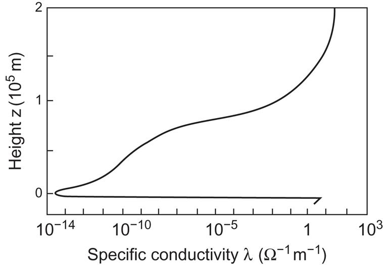
The fair weather downward current of 10−12 A m−2 builds up a negative charge on the surface of the Earth, the total value of which on average is around 105 C. Locally, in the thunderstorm regions, the current is reversed and much more intense. Together, the currents constitute a closed circuit, the flow through which is 500–1000 A, but in such a way that the downward path is dispersed over most of the atmosphere, while the return current in the form of lightning is concentrated in a few regions (apart from being intermittent, causing time variations in the charge at the Earth’s surface). The power P associated with the downward current may be found from
where I (≈10−12 A m−2) is the average current and λ(z) is the conductivity function (e.g., Fig. 3.80 at noon), or more simply from
where C is the capacitance of the Earth relative to infinity (V the corresponding potential difference) and Q (≈105 C) is its charge. The capacitance of a sphere with the Earth’s radius rs (6.4×10⁶ m) is C=4πε0rs=7×10⁻⁴ F (ε0 being the dielectric constant for vacuum), and thus the average power becomes P≈6×10⁻⁵ W m−2.
The energy stored in the charge Q of the Earth’s surface, relative to a situation in which the charges were all moved to infinity, is
In “practice,” the charges could only be moved up to the ionosphere (potential difference less than 106 V), reducing the value of the stored energy by almost two orders of magnitude. In any case, the charge of the Earth, as well as the tropospheric current system, constitutes energy sources of very small magnitude, even if the more concentrated return flux of lightning could be utilized (multiplying the average power estimate by the area of the Earth, one obtains a total power of 3×10¹⁰ W).
3.5 Biological conversion and stores
The amount of solar energy stored in the biosphere in the form of standing crop biomass (plants, animals) is roughly 1.5×10²² J (see section 2.4.1), and the average rate of production is 1.33×10¹⁴ W or 0.26 W m−2. The residing biomass per unit area is small in oceans and large in tropical forests. The average rate of production on the land surface is 7.6×10¹³ W or 0.51 W m−2 (Odum, 1972), and over 0.999 of the standing crop is found on land.
Still larger amounts of dead organic matter are present on the Earth in various degrees of fossilization (see Fig. 2.92, expressed in carbon mass units rather than in energy units; 1 kg carbon roughly corresponds to 41.8×10⁶ J). Thus, fossil deposits (varieties of coal, oil, and natural gas) are estimated to be of the order of 6×10²³ J. This may be an underestimate, in view of the floating distinction between low-concentration energy resources (peat, shale, tar sand, etc.) and non-specific carbon-containing deposits. A maximum of about 1×10²³ J is believed to be recoverable with technology that can be imagined at present (cf. section 2.4.2), suggesting that fossil energy resources are not very large compared with the annual biomass production. On the other hand, converting fresh biomass into useful energy requires more sophisticated methods than are generally required to convert the most pure and concentrated fossil fuel deposits. For bioenergy sources that have been in use for a long time, such as firewood and straw, an important requirement is often drying, which may be achieved by direct solar radiation.
It should not be forgotten that plants and derived forms of biomass serve man in essential ways other than as potential energy sources, namely, as food, as raw material for construction, and—in the case of green plants—as producers of atmospheric oxygen. The food aspect is partially an indirect energy usage, because man and other animals convert the energy stored in plants by metabolic processes that furnish energy required for their life processes. Biomass serving as food also acts as a source of mineral nutrients, vitamins, etc., which are required for reasons other than energy.
Assessment of the possible use of bioenergy for purposes other than those associated with life processes must take into account both biomass’s food role and other tasks presently performed by vegetation and animal stock, such as prevention of soil erosion, conservation of diversity of species and balance of ecological systems. Only energy uses that can be implemented in harmony with (maybe even in combination with) these other requirements can be considered acceptable. Although plant systems convert only a small fraction of incident solar radiation, plans for energy usage should also consider the requirements necessary to avoid any adverse climatic impact. The management of extended areas of vegetation has the potential to interfere with climate, for example, as a result of the strong influence of vegetation on the water cycle (soil moisture, evaporation, etc.). Illustrations of such relations and actual climatic changes caused by removal of vegetation, overgrazing, etc., are given in section 2.4.2.
Before the question of plant productivity in different geographical regions and under different conditions is considered, the biochemistry of photosynthetic processes in green plants is briefly outlined.
3.5.1 Photosynthesis
3.5.1.1 Mechanism of green plant photosynthesis
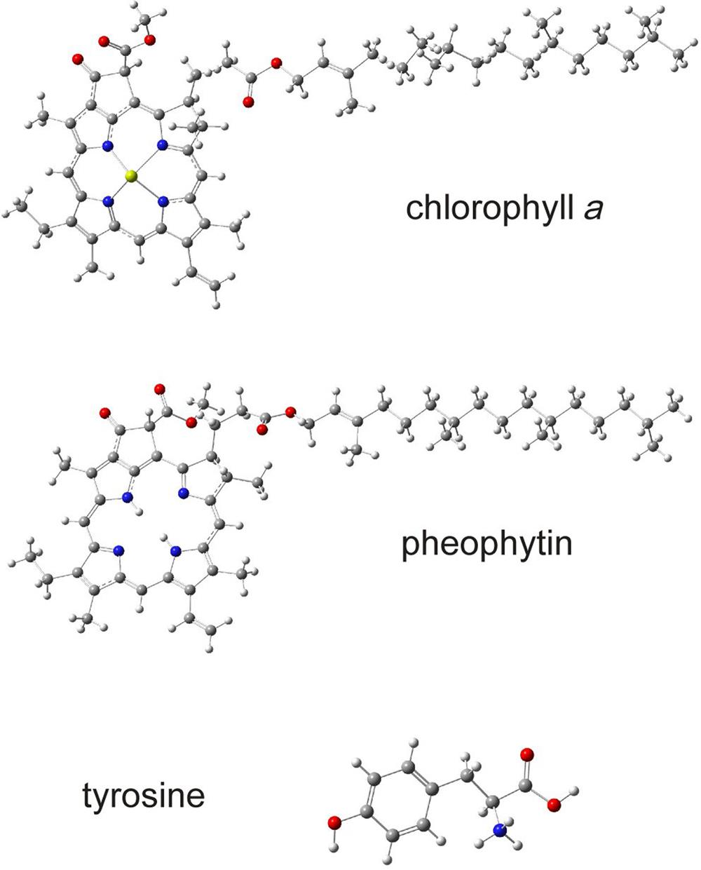
The cells of green plants contain a large number of chloroplasts in their cytoplasm. The interior of a chloroplast contains a liquid, the stroma, rich in dissolved proteins, in which floats a network of double membranes, the thylakoids. The thylakoid membranes form a closed space containing chlorophyll molecules in a range of slightly different forms, as well as specific proteins important for photosynthesis. In these membranes, photo-induced dissociation of water takes place,
(3.40)
and the electrons are transferred, through a number of intermediaries, from the internal to the external side of the membrane. The transport system is depicted in Fig. 3.73, where the ordinate represents the redox potential [the difference in redox potential between two states roughly equals the amount of energy that is released or (if negative) that has to be added, in order to go from one state to the other].
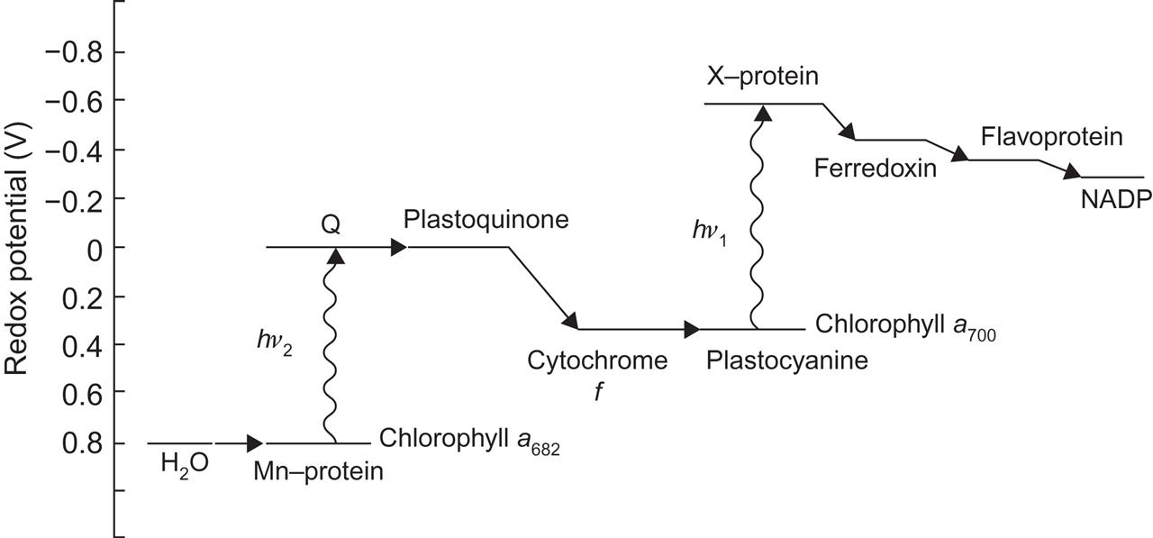
The first step in the reaction is the absorption of solar radiation by a particular chlorophyll pigment (a680). The process involves the catalytic action of an enzyme, identified as a manganese complex, that is supposed to trap water molecules and become ionized as a result of the solar energy absorption. Thereby, the molecules (of unknown structure) denoted Q in Fig. 3.73 become negatively charged, i.e., electrons have been transferred from the water–manganese complex to the Q-molecules of considerably more negative redox potential (Kok et al., 1975; Sørensen, 2005).
The photosensitive material involved in this step is called photosystem II. It contains the chlorophyll pigment a680 responsible for the electron transfer to the Q-molecules, where 680 is the approximate wavelength (in 10−9 m), for which the light absorptance peaks. It is believed that the initial absorption of solar radiation may be affected by any of the chlorophyll pigments present in the thylakoid and that a number of energy transfers take place before the particular pigment that will transport an electron from H2O to Q receives the energy (Seliger and McElroy, 1965).
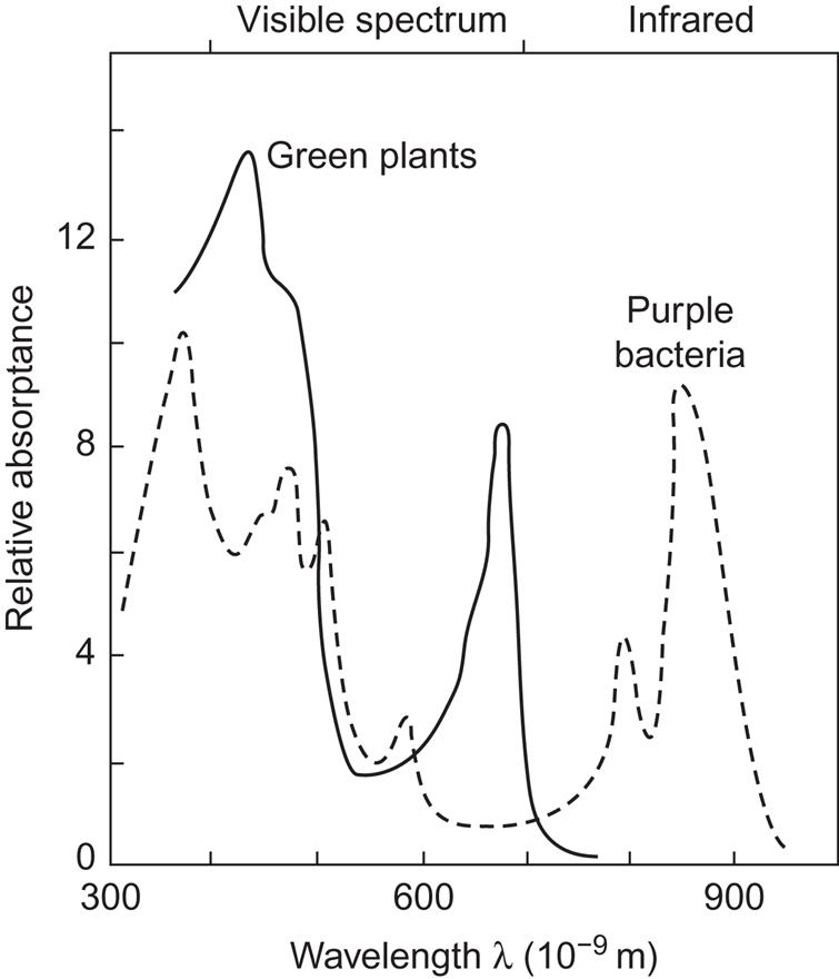
The gross absorptance as a function of wavelength is shown in Fig. 3.74 for green plants and, for comparison, a purple bacterium. The green plant spectrum exhibits a peak just above 400×10−9 m and another one a little below 700×10−9 m. The bacterial spectrum is quite different, with a pronounced peak in the infrared region around 900×10−9 m. The positions of the peaks are somewhat different for the different types of chlorophyll (a, b, c, …), and they also move if the chlorophyll is isolated from its cellular surroundings. For a given chlorophyll type, different pigments with different absorption peak positions result from incorporation into different chemical environments (notably, bonding to proteins).
Returning to Fig. 3.73, the electrons are transferred from the plastoquinone to cytochrome f by a redox reaction, which transfers a corresponding number of protons (H+) across the thylakoid membrane. The electrons are further transferred to plastocyanine, which leaves them to be transported to another molecule of unknown structure, the X-protein. The energy required for this process is provided by a second photo-excitation step, in what is called photosystem I, by means of the chlorophyll pigment a700 (spectral peak approximately at 700×10−9 m).
The electrons are now delivered to the outside region, where they are picked up by ferredoxin, a small protein molecule situated at the outer side of the thylakoid membrane system. Ferredoxin may enter a number of different reactions; a very important one transfers the electrons via flavoprotein to nicotinamide–adenine dinucleotide phosphate (NADP), which reacts with protons to form NADPH2, the basis for carbon dioxide assimilation. The protons formed by (3.40) and by the cytochrome f–plastoquinone reduction are both formed inside the membrane, but they penetrate the thylakoid membrane by a diffusion process, regulated by reaction (3.42) described below. The NADPH2-forming reaction may then be written
(3.41)
which describes the possible fate of electrons and protons formed by process (3.40), after transport by the sequence shown in Fig. 3.73 and proton diffusion through the membrane.
The transport of protons from outside the thylakoid membrane to its inside space, by means of the plastoquinone–cytochrome f redox cycle, creates an acidity (pH) gradient, which in turn furnishes the energy necessary for the phosphorylation of adenosine diphosphate (ADP) into adenosine triphosphate (ATP),
(3.42)
This process, which involves the action of an enzyme, stores energy in the form of ATP (4.8×10⁻²⁰ J per molecule), which may later be used to fuel energy-demanding processes, such as in the chloroplast stroma or in the cytoplasm outside the chloroplast (see, for example, Douce and Joyard, 1977). It is the analogue of the energy-stocking processes taking place in any aerobic plant or animal cells (i.e., cells using oxygen), as a result of the degradation of food (saccharides, lipids, and proteins), and associated with expenditure of oxygen (the respiratory chain, the Krebs cycle; see, for example, Volfin, 1971). The membrane system involved in the case of food metabolism is the mitochondrion.
By means of the energy stored in ATP and the high reducing potential of NADPH2, the CO2 assimilation process may take place in the stroma of the chloroplasts independently of the presence or absence of solar radiation. The carbon atoms are incorporated into glyceraldehyde 3-phosphate, which forms the basis for synthesis of glucose and starch. The gross formula for the process leading to the synthesis of glyceraldehyde 3-phosphate in the chloroplasts (the Benson-Bassham-Calvin cycle; cf. Douce and Joyard, 1977) is
(3.43)
Reactions (3.40) to (3.43) may be summarized,
(3.44)
Going one step further and including the synthesis of glucose, the classical equation of photosynthesis is obtained,
(3.45)
where 4.66×10⁻¹⁸ J is the net energy added by solar radiation.
3.5.1.2 Details of photosynthetic processes
Figure 3.75 shows the components of the photosystems residing along the thylakoid membranes. Insights into the structure of the membrane and component architecture have recently been obtained by atomic force microscopy (Bahatyrova et al., 2004). The space inside the membranes is called the lumen, while on the outside there is a fluid, the stroma, which is rich in dissolved proteins. The whole assembly is in many cases enclosed within another membrane defining the chloroplasts, entities floating within the cytoplasm of living cells, while in some bacteria there is no outer barrier: they are called “cell-free.”
Although some of the basic processes of photosynthesis have been inferred long ago (see Trebst, 1974), the molecular structures of the main components have only recently been identified. The reason is that the huge molecular systems have to be crystallized in order for spectroscopy, such as X-ray diffraction, to be used to identify atomic positions. Crystallization is achieved by a gelling agent, typically a lipid. Early attempts either damaged the structure of the system of interest, or used a gelling agent that showed up in the X-rays in a way difficult to separate from the atoms of interest. Very slow progress finally resulted in discovery of suitable agents and improvement of the resolution, from an initially more than 5 nm down to approximately 0.8 nm by 1998 and then recently to about 0.2 nm. The improved resolution allows most of the structure to be identified, although not the precise position (e.g., of hydrogen atoms). In the future, it is expected that the actual splitting of water may be followed in time-slice experiments under pulsed illumination.
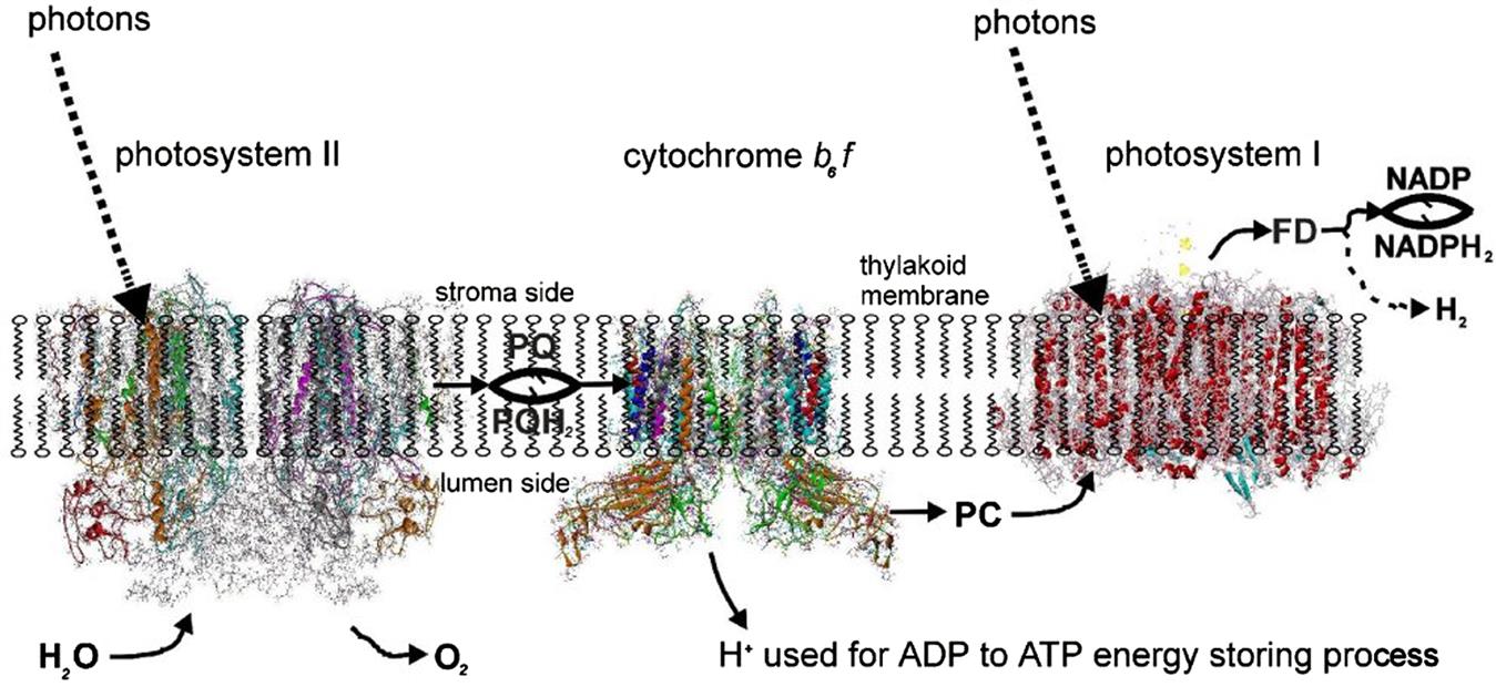
Figure 3.75 places the main photosystems along the thylakoid membrane, shown schematically but with the three systems exhibiting extrusions on the luminal or stromal side according to experimental findings. The splitting of water by solar radiation takes place in photosystem II (PS II), with hydrogen emerging in the form of pqH2, where pq is plastoquinone. Cytochrome b6 f (which resembles the mitochondrial cytochrome bc1 in animals) transfers the energy in pqH2 to plastocyanin (pc) and recycles pq to PS II. The plastocyanin migrates on the luminal side of the membrane to photosystem I (PS I), where more trapping of sunlight is needed to transfer the energy to the stromal side of the membrane, where it is picked up by ferredoxin (fd). Ferredoxin is the basis for the transformation in the stroma of NADP to NADPH2, which is able to assimilate CO2 by the Benson-Bassham-Calvin cycle (see (3.43)) and thereby form sugar-containing material, such as glucose and starch. However, a few organisms are capable of alternatively producing molecular hydrogen rather than NADPH2. Selection of the hydrogen-producing process could possibly be managed by genetic engineering. In order to highlight the points where intervention may be possible, the individual processes are described in a little more detail.
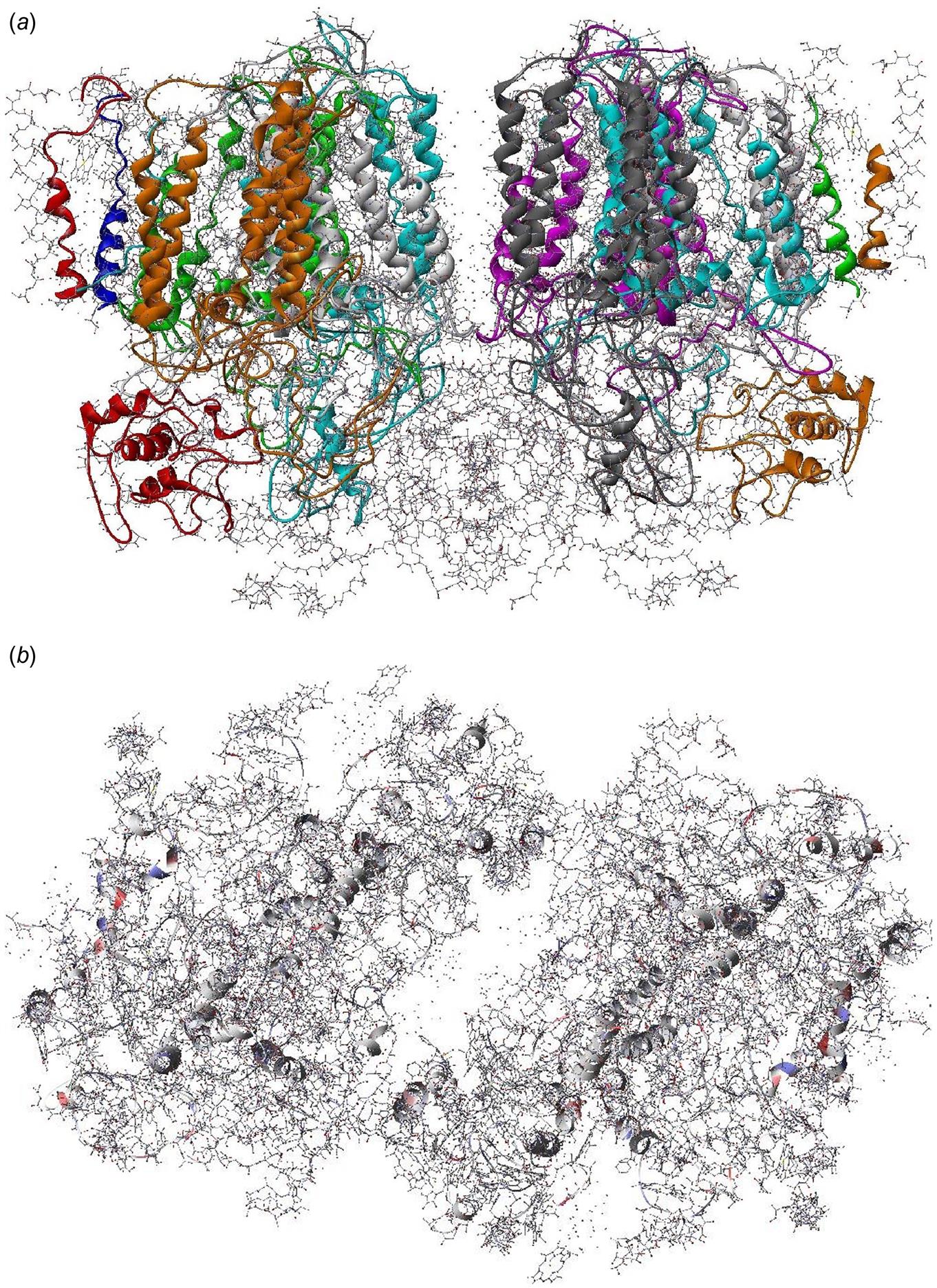
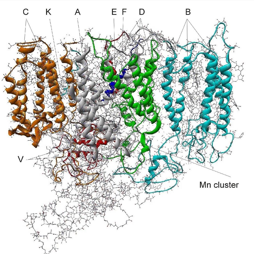
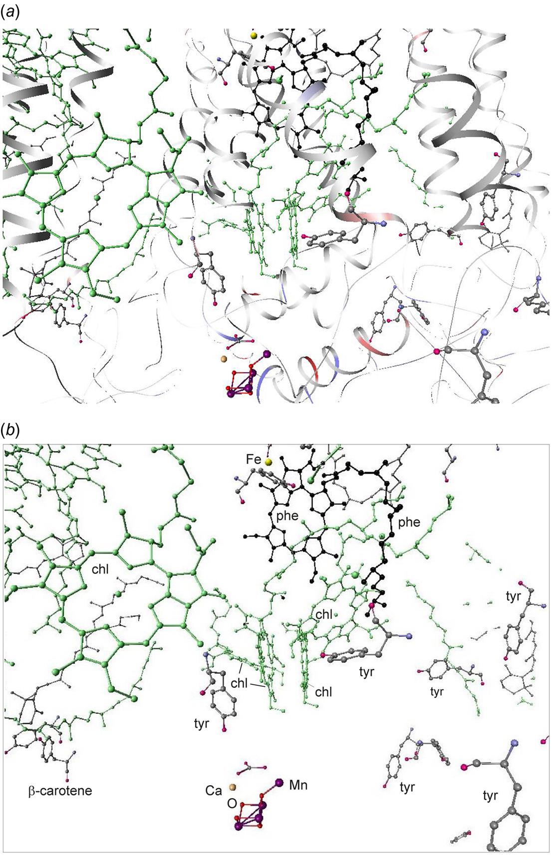
The structure of PS II, which is similar for different plants and bacteria, helps to reveal the mechanisms of light trapping, water splitting, and transfer between sites. Figure 3.76a and b, based on a thermophilic cyanobacterium (Thermosynechococcus vulcanus) show the overall structure of PS II, seen from the side, as in Fig. 3.75, and from the top.* The structure is that of a dimer with two nearly identical parts. If one part is removed and pivoted to orient the “inner” surface (where the interface between the two parts was) directly at the viewer, the remaining monomer is as shown in Fig. 3.77, with a number of amino acid chains indicated as solid helices drawn over the molecular structure. In Fig. 3.78, the view is tilted in order to better display the reaction center details shown in Fig. 3.79. At the 0.37 nm resolution of the X-ray data used, 72 chlorophylls are identified in the PS II dimer. The zoomed monomer picture shows the four central chlorophyll rings (the experiment did not identify the side chains that allow the chlorophylls to attach to the membrane, cf. Fig. 3.80) and the unique manganese cluster of four atoms (there are another four in the other monomer). Manganese serves as a catalyst for the water splitting, as is discussed below. The many chlorophylls are part of an antenna system capable of absorbing solar radiation at the lower wavelength (higher energy) of the two peaks shown in Fig. 3.75 for green plants. The side chains shown in Fig. 3.80 and the long molecules of β-carotene probably also contribute to light absorption, with a subsequent transfer of energy from the initial chlorophyll molecules capturing radiation to the ones located in the reaction center region near the Mn atoms, as indicated in Fig. 3.79.

The present understanding of the working of PS II is that solar radiation is absorbed by the antenna system, including the large number of chlorophyll molecules, such as those of region B in Fig. 3.77, and possibly some of the other molecules, including, as mentioned, the β-carotenes. When absorbed, a light quantum of wavelength λ=680 nm delivers an energy of
(3.46)
where c is the vacuum speed of light (3×10⁸ m s−1) and h is Planck’s constant (6.6×10⁻³⁴ Js). The excited chlorophyll state is a collective state involving electrons in all parts of the central ring structure (not the central Mg atom in particular, as demonstrated by experiments substituting other elements in this position). The excited state may decay and re-emit the energy as a photon (fluorescence), but the probability of transferring the energy to a neighboring chlorophyll molecule is higher. In this way, the energy is handed from one chlorophyll molecule to another until it reaches one of the central chlorophyll-a molecules pointed out in Fig. 3.79b. The arrangement in this region favors a particular set of reactions, summarized in Fig. 3.81.
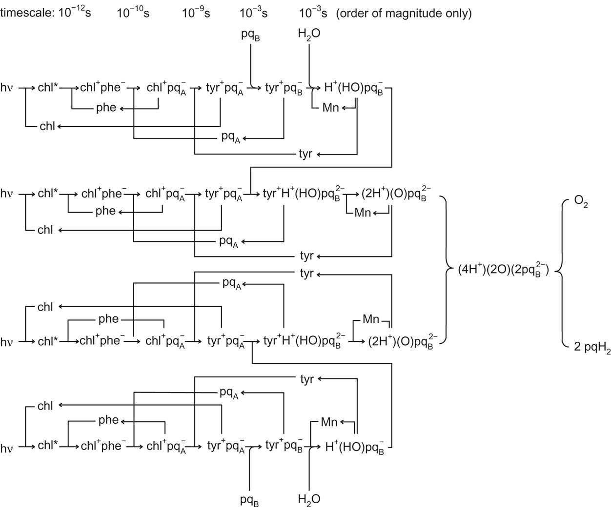
By transferring an electron to pheophytin (one of the two molecules shown in Fig. 3.79b), the donating chlorophyll-a is left in a positively charged state. The pheophytin passes on the electron to a plastoquinone, from which it is passed to a second plastoquinone believed to be better able to form pcH2 and move around, after taking two protons from two of the processes shown in Fig. 3.81, and subsequently migrate from PS II to the cytochrome b6 f complex for the next step shown in Fig. 3.75. The plastoquinone structure is shown in Fig. 3.82, taken from a recent study of the cytochrome b6f complex (Kurisu et al., 2003); only the ring of one of the pq’s is seen in the PS II X-ray studies of Kamiya and Shen (2003) or Zouni et al. (2001). Considerable attention has been paid to identification of the processes by which hydrogen ions are actually removed from water molecules, using 4 quanta of energy from the central chlorophyll absorbers. It has long been suspected that the Mn cluster serves to facilitate such processes, but first, energy has to get from the excited and positively charged chlorophyll molecule into the neighborhood of the Mn atoms. The Mn atoms have double positive charges and the cluster is believed to be held in place by weak forces tying them to some of the amino acids of the nearby A-chain (Fig. 3.79a). The chemical jargon is that the Mn atoms are being “co-ordinated” by the polypeptides of the D1 subunit. The amino acid most likely to donate an electron to the chl+ ring is the ring structure of a tyrosine molecule identified as tyr161 (using the label numbering of the recent experiments quoted). The most recent X-ray experiment has a resolution of 0.35 nm, so there is considerable room for additional structures (and atoms) to be identified as resolution approaches typical atomic distances (around 0.1 nm).
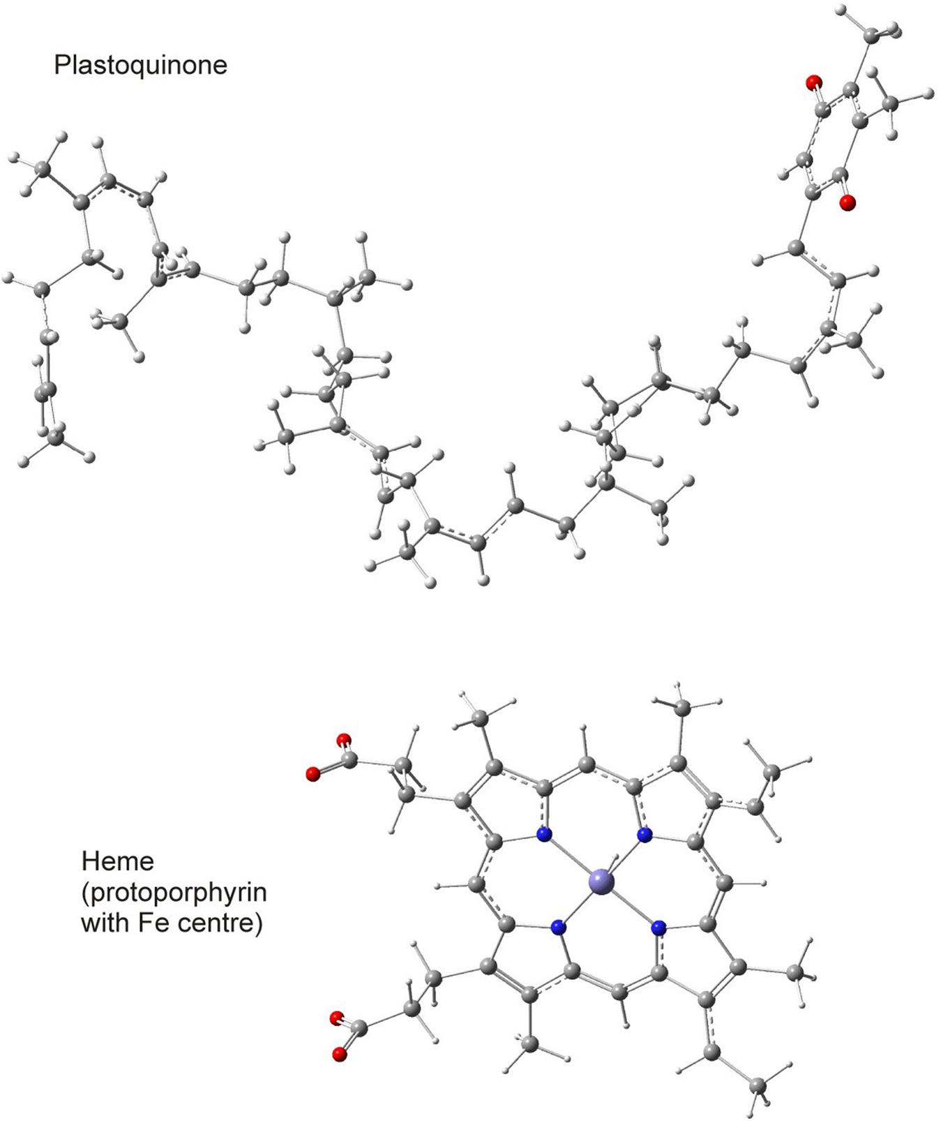
In Fig. 3.81, all four chlorophyll molecules, having received solar energy, transfer an electron via pheophytin to plastoquinone-A and take one from a tyrosine molecule. In the first set of two reactions (top and bottom in Fig. 3.81), a hydrogen atom in a neighboring water molecule is made to transfer an electron to the tyrosine(−161), presumably under the influence of the Mn atoms. In the second set of reactions, the electron transfer from plastoquinone-A to an already negatively charged plastoquinone-B makes this doubly charged, which may also help to rip an electron from the second hydrogen atom in the water molecule. There are now two H+ ions and a pqB molecule with a charge of –2, which combine to form pqH2. The subscript B is now dropped, as it is regarded as an indication of the site of reaction and therefore is irrelevant for a plastoquinone that can move along the membrane to the following process step (in the cytochrome b6 f complex). Finally, the two oxygen atoms left behind by the process will form an oxygen molecule, possibly again under the wings of the Mn catalyst. This understanding of water splitting is consistent with recent structural data, but the matter cannot yet be considered completely settled. Early theoretical explanations use sets of oxides MnOx (with x=2 or more) that change their charge or charge co-ordination state relative to the trapped water molecules, in consort with the one-by-one stripping and release of four protons (H+) and four electrons (e−) (Kok et al., 1970; Hoganson and Babcock, 1997).
The scheme in Fig. 3.81 also allows an interpretation of where the plastoquinones at sites A and B are on equal footing: one is formed by the first reaction line in Fig. 3.81. If the second reaction involves the same pheophytin as the first, it will follow the reaction scheme in line 2 of Fig. 3.81; otherwise, it will follow the scheme in line 4. The remaining two steps are now fixed, provided that the plastoquinones have little probability for harboring more than two negative charges. With the positions of most atoms determined, it should be possible to perform more realistic theoretical calculations of the reaction processes in the near future and thereby verify the status of the proposed reaction paths.
Once the pqH2 reaches cytochrome b6f and gets close to a protoporphyrin heme molecule, the two protons are released and plastoquinone is recycled to the PS II. Figure 3.83 shows the overall structure of the cyanobacterium Mastigocladus laminosus cytochrome b6 f (Kurisu et al., 2003), which, together with the structure derived from the alga Chlamydomonas reinhardtii (Stroebel et al., 2003), is the most recent element in completion of the photosystem structure. Similar functions are performed in animal mitochondria by cytochrome bc1 (Iwata et al., 1998) and in purple bacteria by cytochrome c2 (Camara-Artigas et al., 2001). Figure 3.84 gives details of the b6f components, including three iron-containing hemes in cytochrome b6 and one in cytochrome f, plus the inorganic Fe2S2 molecule serving as an intermediary between the two cytochrome components.
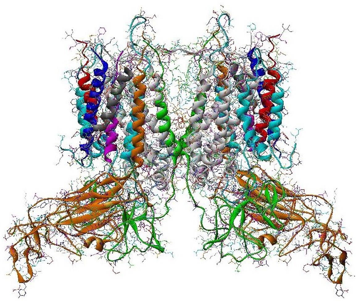
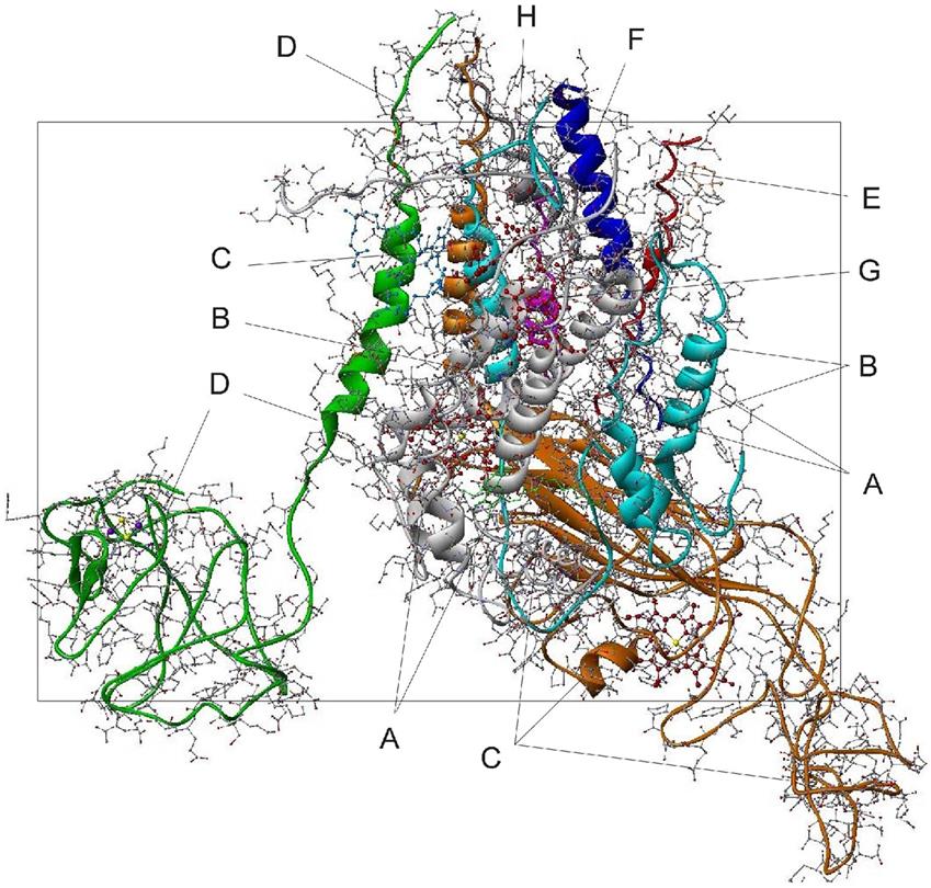
Although as judged from Fig. 3.84 and the blow-up in Fig. 3.85, the Fe2S2 molecule seems too far away to be important, in fact the Rieske protein on which it sits can be turned around the hinge connecting it to the membrane part of the structure and thereby bring the Fe2S2 molecule close to the hemes bL (L for luminal side) and f. The two hemes bH and bS closer to the stromal side are adjacent to a plastoquinone molecule (PL9 in Fig. 3.85) and are thought to accomplish the recycling of pq after the hydrogen ions (protons) have been separated.
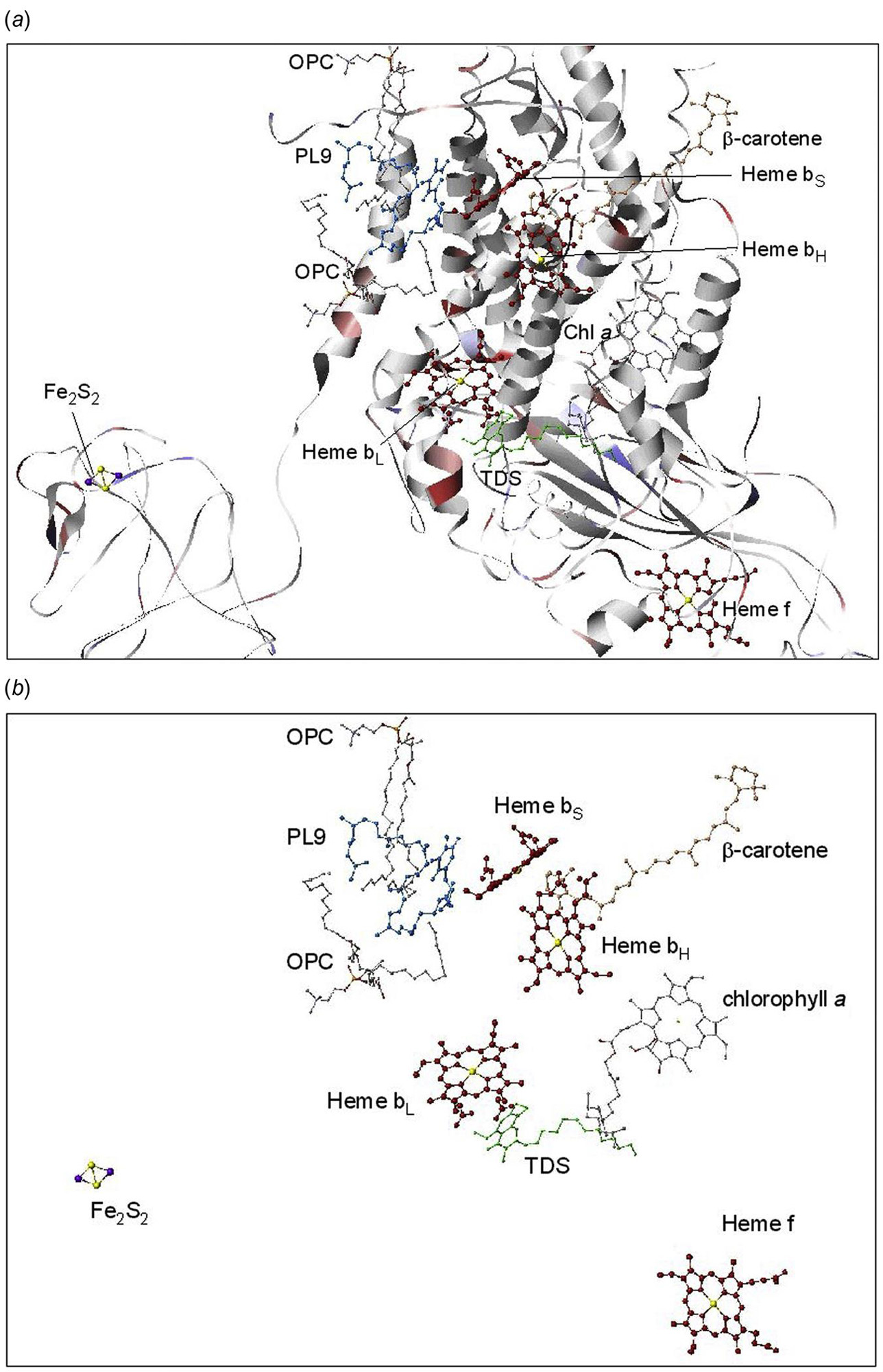
The path via heme f is taken by electrons on their way to the large plastocyanin (pc) molecule occupying a cavity on the luminal side before it moves with the extra electrons to PS I. The rather large pc molecule shown in Fig. 3.86 is from the blue-green alga (another word for cyanobacterium) Anabaena variabilis (Badsberg et al., 1996). Smaller units with only one central Cu atom have been identified, for example, in the plant Arabidopsis, where the role of pc as an electron donor to PS I has been established by measurements indicating a large negative surface electrostatic charge (Molina-Heredia et al., 2003).
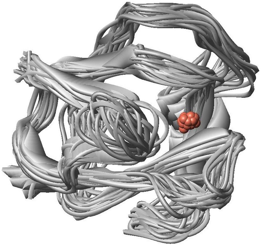
Figure 3.85 also shows a few other molecules identified: TDS (C25H38O5) and OPC (C45H87NO8P), as well as more distant molecules of chlorophyll a and β-carotene. Amino acids from the protein chains (indicated in Fig. 3.85a) help to keep the heme molecules in place and also may facilitate the electron transfer. Transfer of electrons to the luminal side pc with corresponding positively charged hydrogen ions implies the creation of a proton gradient across the membrane. This is where most of the energy transferred from PS II goes, and this energy may be stored for later use by the organism by the process
(3.47)
where ADP and ATP are adenosine di- and triphosphate (structure shown in Fig. 3.87). ATP is formed on the stromal side of the membrane, implying a transport of protons across the membrane.
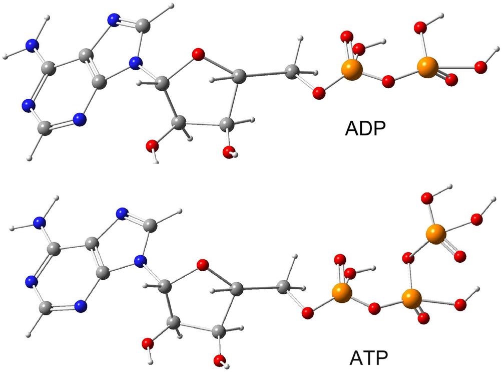
As the next step in photosynthesis, PS I, shown in Fig. 3.88, receives the negatively charged plastocyanin (pc)−1 from cytochrome f, but has to spend energy in transferring electrons across to the stromal side, where they are picked up by ferredoxin for use either in molecular hydrogen formation or for the CO2-assimilating processes of the organism. In order to provide the energy required, PS I contains an antenna system of chlorophyll molecules capable of capturing further solar radiation, albeit at a slightly lower energy than that characterizing the central capture in PS II, corresponding now to wavelengths of about 700 nm.
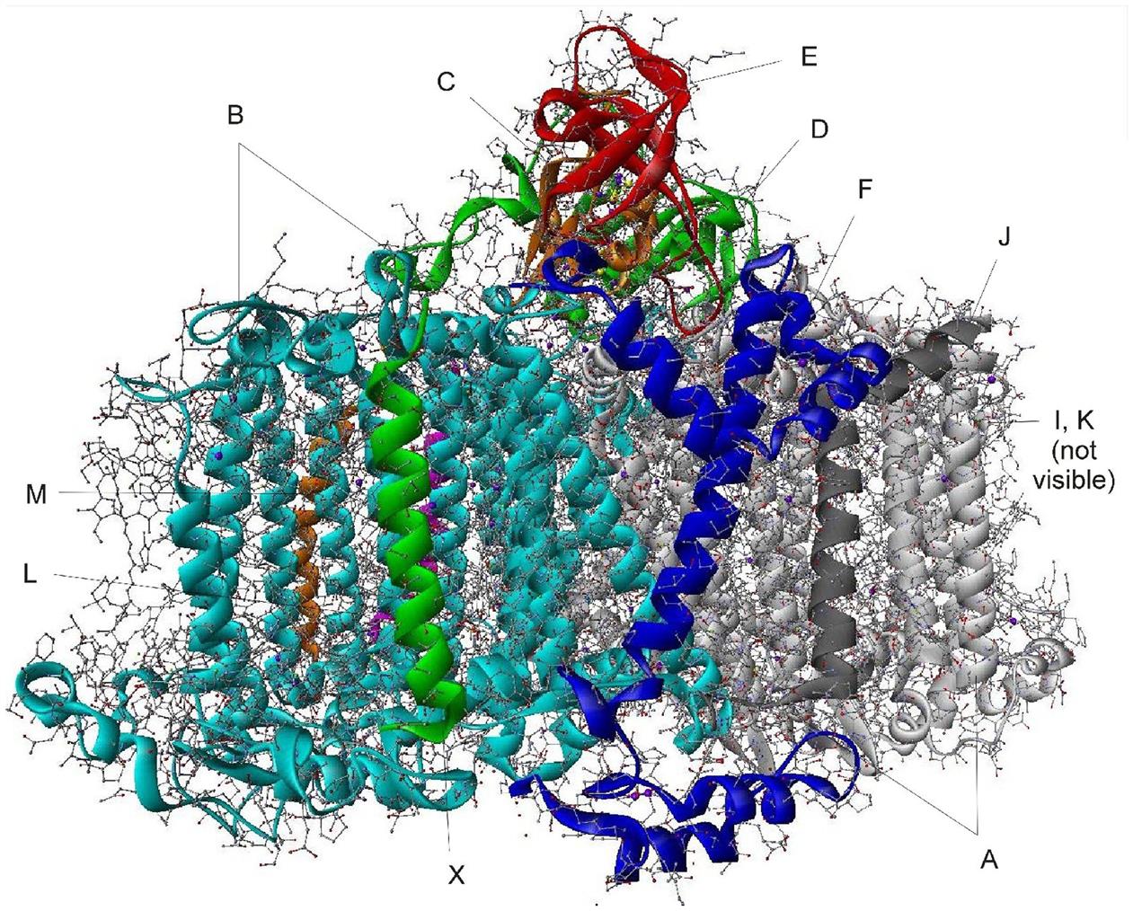
Electrons are brought into PS I from the luminal side, either by plastocyanine pc or, in some cyanobacteria, by cytochrome c6. It has been suggested that plants developed the route with pc and its Cu core at a time in their evolution when Fe was less available in the areas of plant growth (Rosa et al., 2002). Referring to Fig. 3.88, a cavity is seen on the luminal (lower) side, associated with two horizontal helical pieces of subunit F. This cavity, quite close to the chlorophylls chl-A1 and chl-B1 at the beginning of the electron transfer chain (Fig. 3.90), is supposed to be the docking site of cyt-b6 or pc (Fromme et al., 2003). The somewhat surprising presence of a Ca2+ atom on the luminal side (Fig. 3.89a) may have something to do with co-ordination of the three monomers that make up the total PS I (Fromme et al., 2001). The three antenna systems, each with two branches (A and B in Fig. 3.88), consist of a total of 270 chlorophylls (mostly type a, cf. Fig. 3.80), to which come the 3×6 central ones (Fig. 3.90). This very large number (also compared with the 72 chl’s in PS II) is dictated by the fact that PS I must collect solar energy for all the requirements of the organism, whether plant or bacterium.
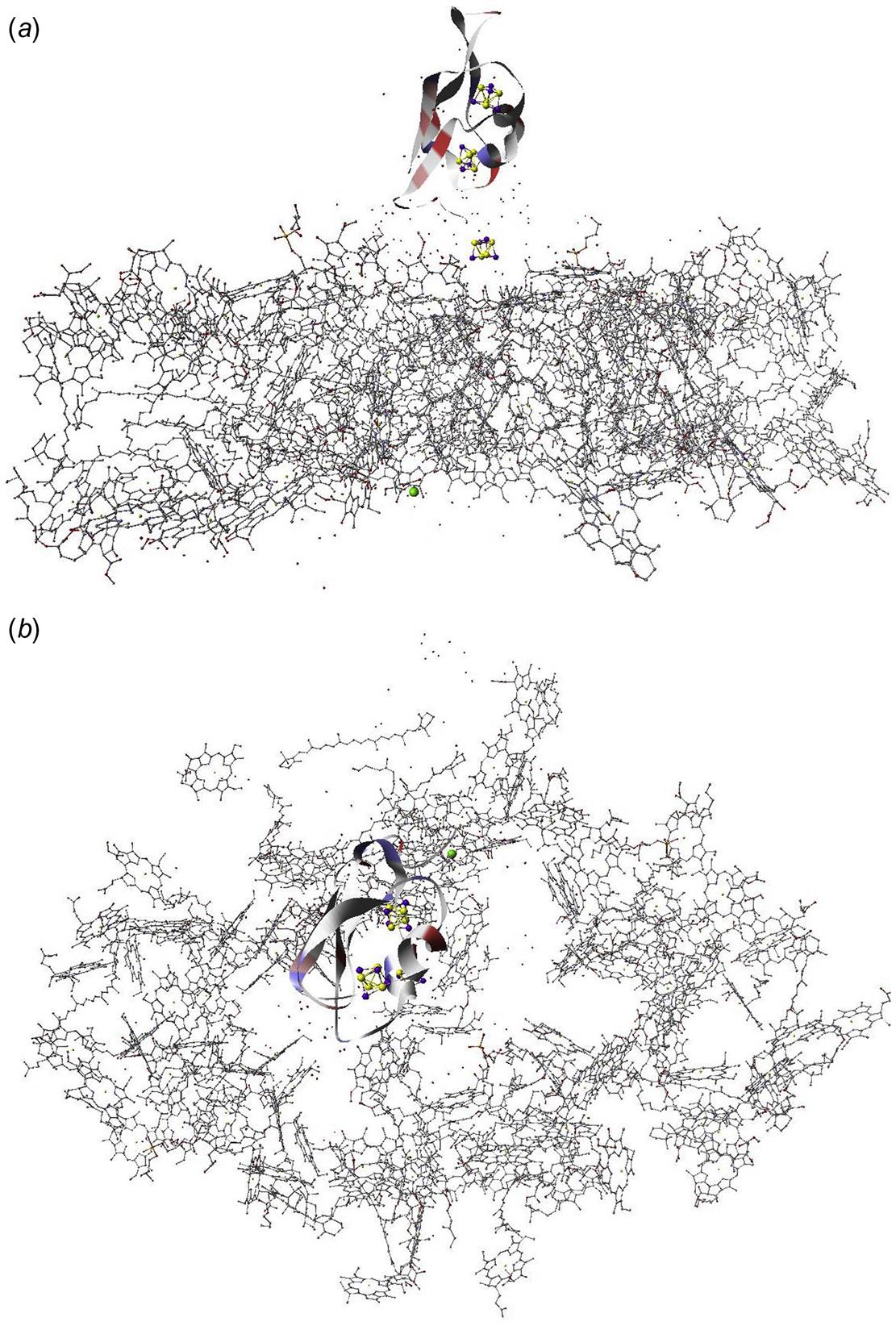
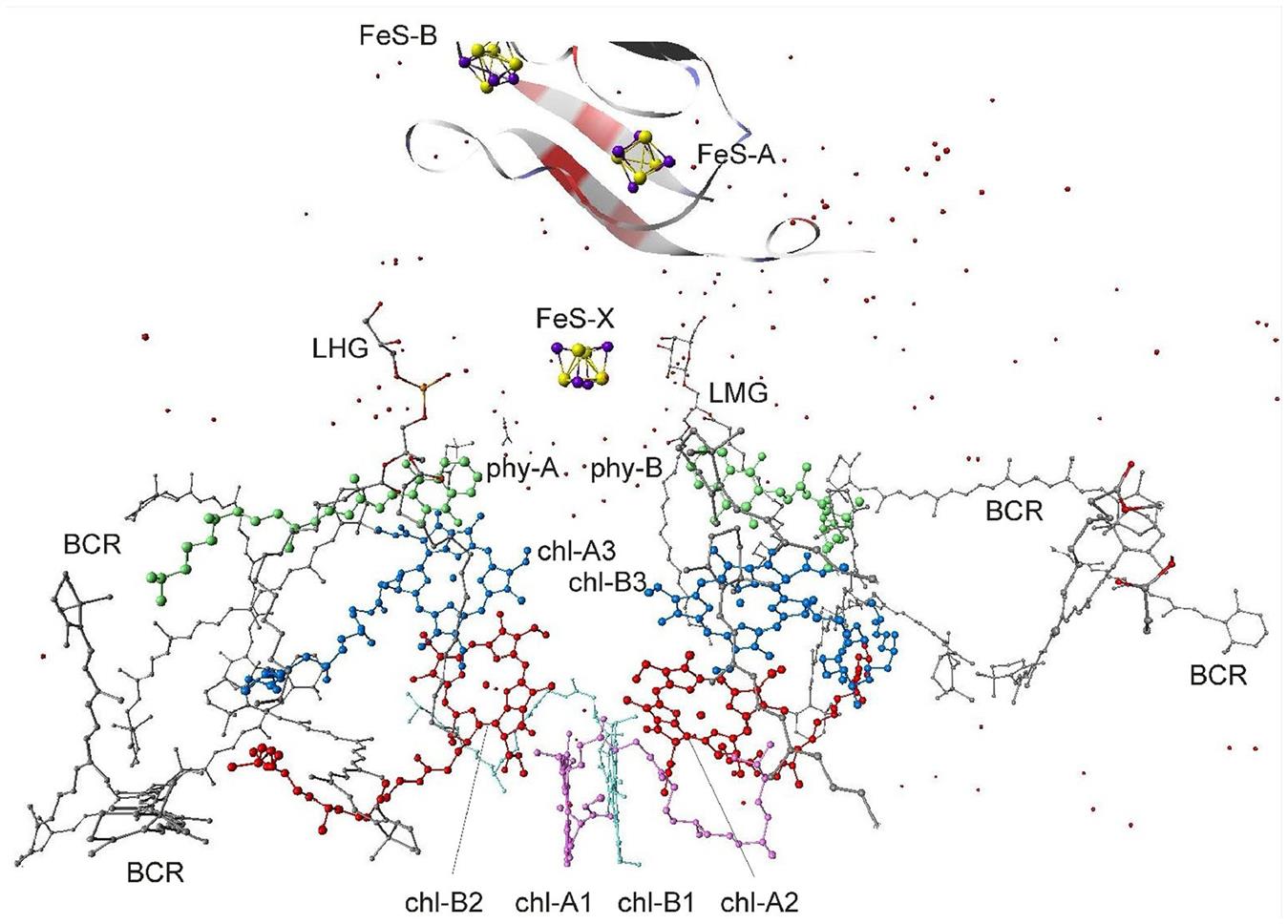
The energy captured from solar energy is transferred from chl to chl in the antennas A and B, until it reaches the central pair [chl-A1, chl-B1] (Fig. 3.90). These two chlorophylls (usually denoted P700) are slightly different in shape and it is not known if both participate in the same manner. An electron is quickly (about 1 ps) passed along one of the vertical paths to chl-A3 or chl-B3. It is not known if it passes through chl-B2 or chl-A2, or if these are parts of the primary collection site P700. In a following rather fast step (some 30 ps), the electron is passed to either phy-A or phy-B, from where somewhat slower processes (20–500 ns) carry the electron successively to the three Fe4S4 molecules FeS-X, FeS-A, and FeS-B. The surrounding amino acid chains play an important role in these transfers (Chitnis, 2001; Brettel and Leibl, 2001). Although charge recombination can occur, the primary electron donor is normally left in a positively charged state P700+ throughout the successive electron transfers to FeS-B. The P700+ (presumably chl-A1 or chl-B1) is brought back to its neutral state by the electron brought into PS I by pc (or cyt-c6) and is then ready for handling the next electron transfer from lumen to stroma.
Unlike PS II, where four light quanta were required in a co-ordinated fashion, due to the energetic requirements for water splitting, PS I may proceed with just a single light quantum of 700 nm or 2.8×10⁻¹⁹ J (1.7 eV). However, this observation does not invite any simple explanation for the dual structure of the central energy transfer chains A and B starting from P700. It could perhaps be that a redundancy was built in during evolution and its use later abandoned.
While the protein chain C surrounding the iron-sulfur clusters (Fig. 3.89) is similar in structure to ferredoxin, it needs a real ferredoxin protein docked on the stromal side to transfer the electron from FeS-B away from PS I. The subsystems C, D, and E on the stromal side of PS I (Fig. 3.88) allow docking not only of the fairly small ferredoxin system (an example of which is shown in Fig. 3.91—there are variations in structure between species, such as plants and cyanobacteria), but also of the larger flavodoxin protein (Fromme et al., 2003), an example of which is shown in Fig. 3.92.

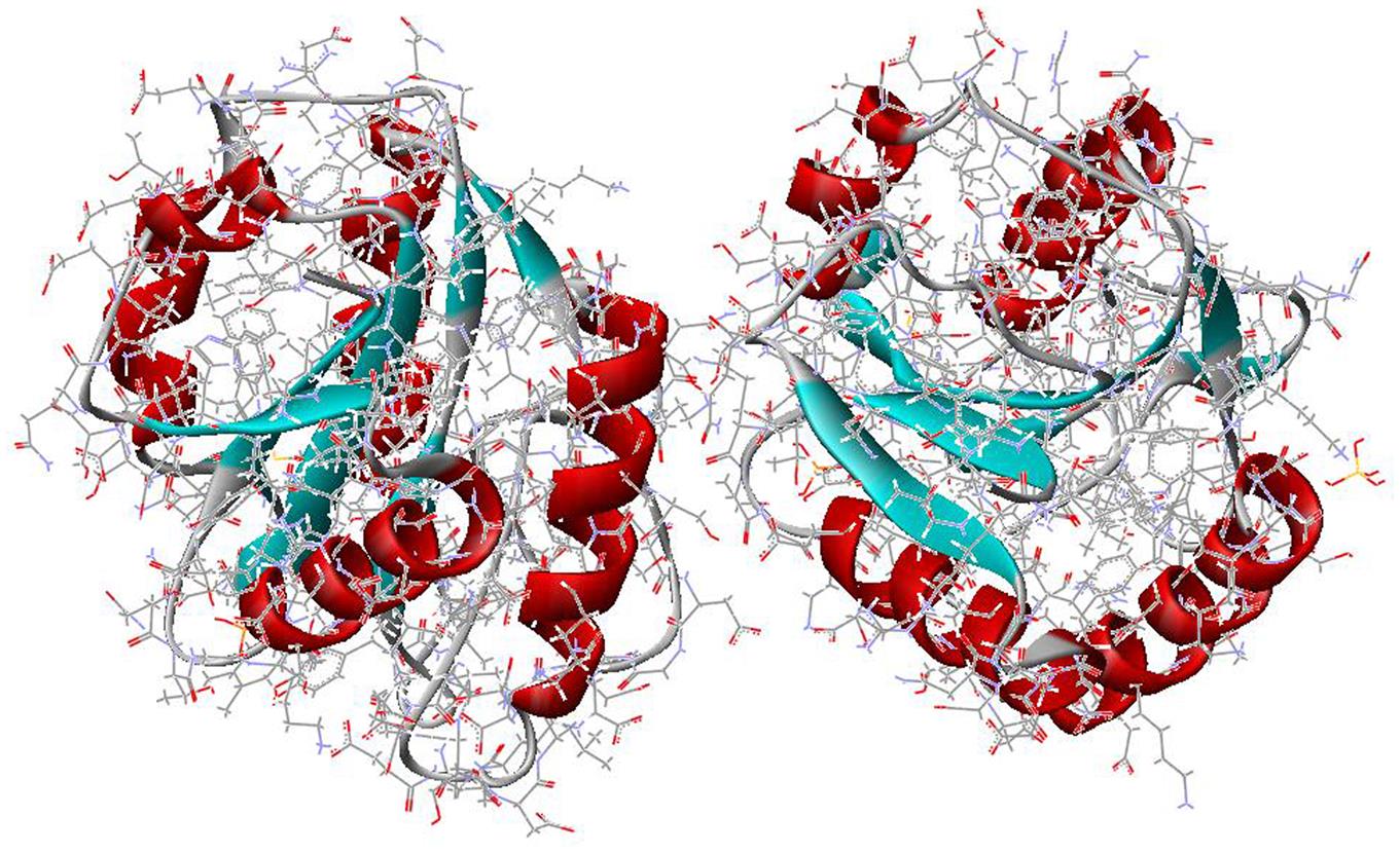
After being brought to the stromal side by the succession of photosystems, a number of electrons are carried by the proteins ferredoxin and flavodoxin. Furthermore, protons (positively charged hydrogen ions) have been separated and moved across the thylakoid membrane (thereby creating an H+ gradient from lumen to stroma). This makes room for two types of recombination processes on the stromal side. One is the “normal” reaction in plants and most bacteria:
(3.48)
where NADPH2 combines with ATP4− from (3.47) and water to assimilate CO2 from the atmosphere for the synthesis of sugars and other molecules needed for the organism in question (see Sørensen, 2005). The second possibility is to induce (e.g., by genetic manipulation) the plant to produce and export molecular hydrogen by some process equivalent to
(3.49)
where, just as in the similar inorganic case, an “agent” (in the inorganic case, a catalyst) is needed for promoting the reaction. In the organic case, the agent may be hydrogenase.
3.5.1.3 Efficiency of conversion
The basis for energy utilization has traditionally been the undifferentiated biomass produced. Other possibilities would include the direct dissociation of water by the action of sunlight (photolysis), or the formation of hydrogen rather than NADPH2, after the initial oxygen formation (3.40) and electron transport to ferredoxin (Benemann and Weare, 1974; Mitsui and Kumazawa, 1977),
(3.50)
In both cases the problem is to control the recombination process,
(3.51)
so that the energy-releasing process takes place where desired and not immediately on the formation of hydrogen. Plants accomplish this by means of the thylakoid membrane and later by the chloroplast external membrane. Man-made processes may attempt to copy the membrane principle in various ways (Broda, 1975; Calvin, 1974, 1977; cf. Chapter 4), but it is not clear that present suggestions will allow separation of hydrogen and oxygen on a large scale. It may be advantageous to use green plants to perform the first step (3.40) and to transport electrons and protons (hydrogen ions) through their membranes; to prevent the energy from being too deeply trapped in organic matter, a strong reducing agent could be added to ferredoxin, as well as suitable enzymes, in order to accomplish the reaction (3.50) at this stage.
The maximum theoretical efficiency of this process is the ratio between the heat release 9.47×10⁻¹⁹ J in (3.51) and the solar energy input required. The latter depends on the absorption properties of the plant and its chlorophyll molecules (cf. Fig. 3.74), as well as on the number of light quanta required for each molecular transformation (3.40). The energy, E, of each light quantum of wavelength λ may be found from
The minimum number of quanta required to transport one electron, as depicted in Fig. 3.73, is 2, one of wavelength 680×10−9 m and the other of 700×10−9 m (although these need not be the quanta originally absorbed). Since (3.40) requires the transport of four electrons, the minimum requirement would be 8 quanta with a total energy of 2.3×10⁻¹⁸ J. Experimental estimates of the number of quanta needed typically give values between 8 and 10.
The efficiency of the photosynthetic process containing only steps (3.40) and (3.50) may be written
(3.52)
where ηλ is the fraction of the frequencies in the solar spectrum (depending on cloud cover, etc.) that is useful in the photosynthetic process, ηgeom is the geometrical efficiency of passing the incoming radiation to the chlorophyll sites (depending on penetration depth in leaves, on reflectance from outer and inner surfaces, and on absorption by other constituents of the leaves), and ηchem is the efficiency of the photochemical reactions, the maximum value of which is given by
This efficiency pertains to the amount of internal heat produced by (3.51). Only a part of it can be converted into useful work. This part is obtained in (3.51) by replacing the enthalpy change 9.47×10⁻¹⁹ J with the change in free energy, ΔG=7.87×10⁻¹⁹ J (cf. section 4.1.1). This way, the efficiency of the photochemical reaction becomes
The efficiency ηλ associated with the chlorophyll absorption spectrum typically lies in the range 0.4–0.5 (Berezin and Varfolomeev, 1976), and the geometrical efficiency ηgeom may be around 0.8 (for the leaf of a green plant, not including the reduction associated with the penetration of radiation through other vegetation, e.g., in a forest environment).
The overall maximum efficiency of about η′≈0.14 found here for a hypothetical hydrogen (H2)-producing system is valid also for actual green plants that assimilate CO2. Over extended periods of time, the biomass production efficiency will have to incorporate still another factor, ηresp, expressing the respiration losses associated with the life cycle of the plant,
(3.53)
The respirative energy losses emerge as heat and evaporated water, at rates depending on temperature and wind speed (Gates, 1968). The value of ηresp is 0.4–0.5 for land plants and somewhat larger for aquatic plants and algae.
Actual plants may get close to the theoretical maximum efficiency, although the average plant does not. For the blue-green alga Anacystis nidulans, Goedheer and Hammans (1975) report an energy efficiency of ηchem≈0.30, based on 36 h of growth, including 6 h of irradiation, with a generous supply of nitrogen and other nutrients, as well as a CO2-enriched atmosphere (i.e., 73% of the maximum energy efficiency calculated above).
It is estimated that, on average, each CO2 molecule in the atmosphere becomes assimilated in a plant once every 200 years and that each O2 molecule in the atmosphere is “renewed” through a plant once every 2000 years (Seliger and McElroy, 1965).
3.5.1.4 Bacterial photosynthesis
Several bacteria use solar radiation to dissociate a compound of the general form H2X, with a net reaction scheme of the form
(3.54)
(Niel, 1941). Here (CH2O) should be understood not as free formaldehyde, but as part of a general carbohydrate compound in analogy to the more precise equation (3.44). Actually, (3.54) was proposed to be valid for both green plant and bacterial photosynthesis, but there is no detailed analogy, since bacterial photosynthesis has been found to take place in a single step, resembling PS I of the green plant two-step process. Other photo-induced reactions do take place in bacteria, connected with ATP formation, which in this case is not a side-product of the primary photosynthetic process.
The compound H2X may be H2S (sulfur bacteria), ethanol C2H5OH (fermentation bacteria), etc. Most photosynthetic bacteria are capable of absorbing light in the infrared region (wavelength 800–1000×10−9 m). The role that the NADP–NADPH2 cycle (3.41) and (3.43) plays for green plant photosynthesis is played by NAD (nicotinamide-adenine dinucleotide)–NADH2 for photosynthetic bacteria. The redox potential of NADH2 is more or less the same as that of the initial compounds, e.g., H2S, so practically no energy is stored in the process of bacterial photosynthesis (Hind and Olson, 1968).
3.5.2 Productivity in different environments
3.5.2.1 Ecological systems
The gross primary production of a plant or, in general, of an ecological system is the rate at which solar energy is assimilated, i.e., the total amount of energy produced by photosynthesis. The net primary production, on the other hand, is the difference between gross primary production and respiration. Respiration involves an increase in redox potential (oxidation), either by consumption of oxygen [aerobic respiration, the net result being equivalent to (3.51)] or by the action of some other agent of oxidation (anaerobic respiration; if the oxidant is an organic compound, the respiration process is called fermentation).
Primary producers are part of an ecological system. Figure 3.93 gives a schematic view of the energy and matter flow through such a system. The primary chain comprises the primary producers capable of carrying out photosynthesis, plant-eating organisms (herbivores), and a chain of successive carnivorous predators (carnivores), some of which may also eat plants (as man does). Each compartment in the chain is called a trophic level, and photosynthetic organisms are called autotrophs, while the consuming organisms further along the chain are called heterotrophs. Over short periods of time, withering and death of autotrophs can be neglected, and the net primary production available to the heterotrophic part of the community equals the gross primary production less the respiration of the autotrophs. Over longer periods, respiration, predation, and death must be considered in order to describe the amounts of biomass in each compartment (standing crop). Generally, biomass diminishes along the chain, but owing to the different average lifetimes, which are often longest for the highest trophic levels of the food chain, the biomass at a given time may be maximal for, say, the second or third member of the chain. Also, the seasonal dependence of primary production in most geographical regions, in conjunction with the short lifetimes of the autotrophs, leads to biomass distribution with a much increased long-range stability in the higher levels. The stability depends on the age of the ecosystem. A young system has fewer species and is more sensitive to external disturbances (climate variations, immigration of new predator species, etc.), which may destroy the food basis for the higher trophic levels. Old ecosystems are characterized by higher diversity and, therefore, are better equipped to circumvent sudden changes in external conditions, at least for a while.
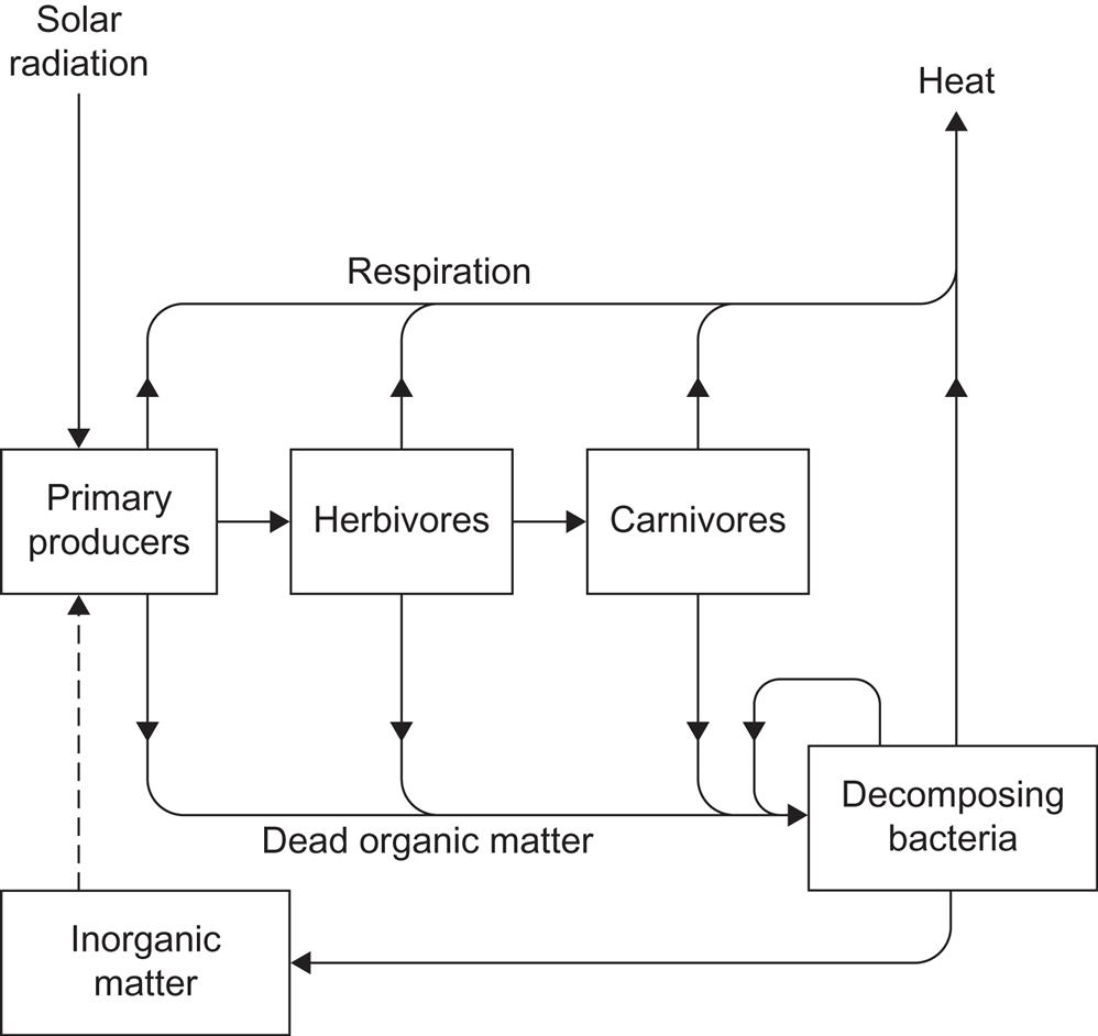
Dead organic matter may precipitate toward the sea floor or detrital layer of the land surface, where an environment suitable for sustaining a number of decomposer bacteria evolves, so that nutrients are returned to the inorganic form necessary for renewed uptake by autotrophs.
It follows from Fig. 3.93 that the flows of energy that could be used for energy extraction serving human society diminish along the food chain. This does not negate the possibility that the concentration of energy flow may be higher and easier to utilize at a level higher than the primary producers. For example, livestock leave a large fraction of their respiration heat and manure within their sheds, a spatial region much smaller than the size of a grazing range that might yield the same energy value.
Important factors in determining the net productivity of a given autotrophic system are solar radiation, temperature regime, water availability, climate in general, and access to carbon dioxide and nutrients, as well as the nature of the entire ecosystem, density and structure of plants in the neighborhood, and predation and harvesting by heterotrophs (including man). Growth in biomass would be exponential if optimal conditions for photosynthesis could be maintained indefinitely. Actual growth is stopped when one or more of the conditions can no longer be met; factors responsible for halting the exponential growth are called limiting factors. A mature ecosystem may reach a stable situation in which the net production (and hence growth) of the community as a whole is zero.
3.5.2.2 Limiting factors
The effective area of a plant that is exposed to solar radiation depends on shadow effects caused by other vegetation and on the shape and arrangements of leaves, or, more generally, of light-absorbing pigments. This, together with the loss caused by scattering and absorption on the leaf surface or other parts of the plant not involved in light accumulation, accounts for the value of the maximum geometrical efficiency in (3.52)—around 0.8. The effective area of fully developed terrestrial plant systems (e.g., forests, erect-leaved cereal crops) is large enough to intercept practically all incident radiation (Loomis and Gerakis, 1975), and most of the losses in these systems are due to reflection.
The availability of solar radiation itself is, of course, very important. (The geographical distribution of radiation is discussed in connection with Fig. 2.24 and in section 3.1.) The penetration of radiation through depths of water is illustrated in Fig. 2.30. The corresponding distributions of productivity for typical coastal and oceanic regions of the North Atlantic are shown in Fig. 3.94. Total autotrophic plus heterotrophic biomass at these sites was found to be 167×103 J m−2 (coastal region) and 8×10³ J m−2 (open ocean) (Odum, 1972).

Excessive solar intensity can diminish efficiency, if the chlorophyll pigments are unable to absorb it all or if the radiation destroys the chlorophyll. Also, the state of the photosynthetic systems as well as of the further energy conversion and transport system of the plant may play a role. Efficiency may be lowered by damage or aging of such components (Wassink, 1975).
If changes do not occur too rapidly, many plants are capable of a measure of adaptation to external conditions of light and humidity, etc. The pathway of carbon synthesis described in section 3.5.1 involves a molecule (3.40) with three carbon atoms (C3-pathway). Some plants are able to follow a different pathway, in which four carbon atoms are synthesized (C4-pathway), notably as malic acid (HO2CCH:CHCO2H). In this case, less CO2 is needed for synthesis of, for example, sugar, so that C4-plants may grow more rapidly than C3-plants, at least in some environments.
Temperature plays an important role: the temperature of both air and soil for terrestrial plants and the temperature of water for aquatic plants. The life cycles of aquatic plankton and algae are relatively short, and for some species, biomass production is confined to a few weeks of the year. Many terrestrial plants are dormant during cold periods, and they are able to withstand low temperatures during winter. If, however, sudden frost occurs in the middle of a growth period, their tolerance is often low and damage may result. For each species, the number of days during the year with temperatures above certain values may be defined as the growing season, a concept that has been used extensively in estimates of average productivity. A phenomenological treatment of the influence of thermal conditions on plant and animal life may be found in the work of Budyko (1974).
Figure 3.95 shows the trends in gross primary production of an evergreen oak forest, along with temperature and average solar radiation. The dashed line gives the net production of the community as a whole (trees and canopy), i.e., the surplus or growth rate, which is high most of the year (except in summer), with peaks in spring and autumn. This is an example of a growing ecosystem. If human intervention can be achieved without changing the trophic relationships within the community, it would appear that a harvest (energy extraction) corresponding to the net production could be sustained, leaving a stable ecosystem with no growth. Man would enter as an additional loop in the system depicted in Fig. 3.93, and the ecosystem would provide a truly renewable energy source.
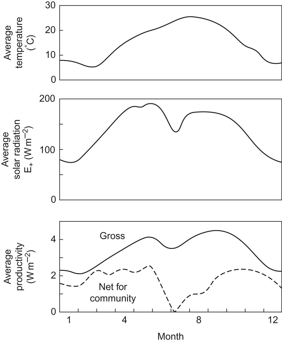
When the standing crop biomass is small, only a small fraction of solar radiation is intercepted. Thus, productivity initially increases with increasing biomass until a turning point of optimal growth conditions is reached, as seen in Fig. 3.96. After this point, productivity slowly decreases toward equilibrium (zero).
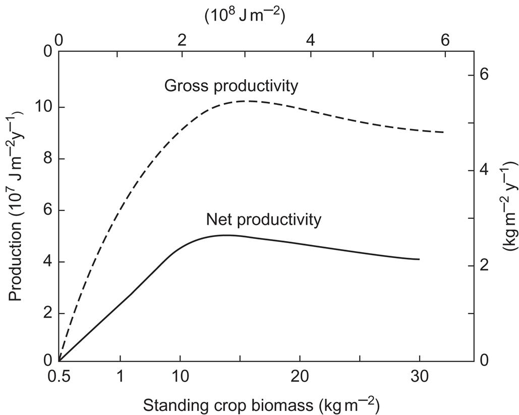
Water flows through all plants at average rates much higher than the rate at which water is dissociated by the first photosynthetic step (3.40). Extra water is required for the oxidation of the manganese enzyme involved in this process, as well as for the cyclic ADT–ATP and NADP–NADPH2 processes, but these amounts of water are not consumed. The same is true for other metabolic processes in the plant, and water also performs physical tasks, such as keeping the surfaces of membranes wet and transporting dissolved substances.
The overall photosynthetic process (3.45) requires one water molecule for each carbon atom assimilated, or 1.5 kg of water for each 1 kg of carbon or for each 42×106 J of biomass, corresponding to 2–3 kg of dry matter. The wet weight is typically 4–10 times the dry weight, implying that the total water content of the plant is at least four times the amount fixed by photosynthesis (and typically is much higher).
The transport of water through a terrestrial plant is achieved by a free-energy gradient, often referred to as the water potential [cf. (3.36) and Canny (1977)]. The corresponding force may thus be more general than that associated with osmotic pressure. Loss of water by transpiration can be viewed as a local decrease in water potential near the area where water is leaving the plant. This means that a potential gradient has been established that will attract water from other parts of the plant. Therefore, the potential gradient moves through the plant and builds up in the root system, which then attracts water from the surrounding soil. If the water that can be drawn from the soil is insufficient, the plant will try to decrease its transpiration by contracting the stomata (openings at leaf surfaces). If the water deficit produces a strong and prolonged stress on the plant, the stomata will become tightly closed, in which case subsequent water saturation will not immediately lead to a complete resumption of photosynthesis at the previous rate (as illustrated in Fig. 3.97).

The turnover of water associated with a biomass production of 1 kg of dry matter is quoted as lying in the range 200–900 kg of water, with values around 500 kg being typical for grass and cereal crops (Geiger, 1961; cf. also Penman, 1970, which quotes 400 kg for food crops).
As an upper limit on the flow of water available to terrestrial plants, one may take the total land precipitation rate of 1.1×10¹⁷ kg of water per year (Fig. 2.65). Assuming the plants’ requirement to be 500 kg of water per kg of dry matter per year, one deduces a maximum sustainable production of 2.2×10¹⁴ kg of dry matter per year, or, in energy units, 4.0×10²¹ J y−1 (1.3×10¹⁴ W).
Since the total terrestrial gross primary production is presently 7.6×10¹³ W (Odum, 1972), and the net primary production may amount to about half this value, it is clear that a large fraction of the evapotranspiration (6.7×10¹⁶ kg of water per year according to Fig. 2.65) over land is due to plants. Accordingly, a substantial increase in terrestrial plant production would have to involve increased recycling of water on time scales shorter than 1 year. One might consider achieving this by artificial irrigation, using some of the water run-off from land areas (3.9×10¹⁶ kg of water per year according to Fig. 2.65). However, as Fig. 2.98 shows, about 70% of the water diverted to food crops is not immediately returned to run-off streams. In view of the many other important functions performed by the rivers and streams responsible for run-off, this suggests that there may be little room for expanding terrestrial biomass production on a worldwide scale if fresh-water resources alone are used for irrigation.
Therefore, schemes for ensuring quick recycling of water added from any source are as important as expansion of the irrigation potential, and furthermore, really significant increases in biomass production must involve oceanic water resources, either by marine biomass production or by use of (eventually distilled) seawater for irrigation. Some terrestrial plants actually accept seawater irrigation, with some reduction in conversion efficiency (Epstein and Norlyn, 1977).
If the availability of CO2 is the only limiting factor, it is reasonable to assume that productivity is proportional to the amount of CO2 entering the plant. The concentration X of CO2 at the photosynthetic sites may be related to the atmospheric CO2 concentration Xatm, expressed as a linear relation
where f depends on properties of the plant (inside pressure, opening of stomata, etc.), as well as on the CO2 eddy diffusion parameter in the air surrounding the plant. The atmospheric concentration Xatm decreases with height when no photosynthesis takes place (night condition), as shown, for example, in Fig. 2.33. However, during daytime in low wind conditions, the CO2 concentration exhibits a minimum halfway through the canopy of vegetation (Saeki, 1975).
If the proportionality factor between production P and CO2 internal concentration X is g, when no other limiting factors are encountered, then the rate of primary production as function of incident radiation, E+, may be written
(3.55)
where η′ (3.52) is the efficiency at low incident radiation, when light is the only limiting factor. In (3.55), temperature requirements are assumed to be satisfied, and the water and nutrient supply are assumed to be adequate.
The state of the photosynthetic system within the plant may give rise to different efficiencies ηchem under different conditions. Basically, this can be understood in terms of competing pathways for the chain of molecular reactions involved. In the electron transport chain, Fig. 3.73, the Q to plastoquinone electron transport in PS II may have to compete with fluorescent de-excitation of the Q-molecule. A similar de-excitation of the X-protein may occur in PS I. In both cases, the energy captured by the chlorophyll pigments will be unavailable to biomass production. In summary, under less-than-optimal conditions, more than 8 light quanta are required for each CO2 molecule assimilated (the excess energy being lost as heat or radiation).
In aquatic environments, the rate of photosynthesis may depend on such factors as salinity and pH value (acidity). It has been suggested that the decreased productivity of coniferous forests in Sweden is associated with increasing acidity of precipitation (and hence of soil) (Swedish Ministries of Foreign Affairs and of Agriculture, 1971).
Last, but not least, the role of nutrients as a limiting factor should be mentioned. Deprivation of nutrients decreases and eventually halts production. Transfer of plants to nutrient-free environments has shown effects of decreasing magnitude resulting from deprivation of nitrogen, phosphorus, and potassium, in that order.
It follows from Figs. 2.92 and 2.93 that an average of 1.4×10⁻³ kg of nitrogen is fixed for each kg of carbon fixed in the terrestrial biosphere, in which there is about 0.0343 kg of N (kg of C)−1 (the standing crop biomass shows a different relationship between N and C, owing to different turnover times). The amount of nitrogen with which the soil must be enriched in order to increase productivity, if N is a limiting factor, may be much larger, owing to the nature of the pathways of uptake. Delwicke (1970) quotes experiments in which 0.76 kg of N was needed in order to increase production by 1 kg of dry matter.
In evaluating the net energy yield of cultivated land or sea, non-solar energy subsidies must also be considered. These may be in the form of machinery and fuels for running the machinery (plowing and harvesting tools). In the present day practice of terrestrial agriculture, the largest energy subsidy in areas of intense farming is in the manufacture of fertilizers. In regions demanding irrigation, water pumping may expend substantial amounts of energy, whereas the amount of machinery employed typically is large only in regions of intense farming, so that the corresponding energy subsidy remains a fraction of that spent on fertilizer. If little machinery is used, more manpower is needed, combined with power provided by draught animals. Also, transport of harvested crops costs energy, particularly for remote fishing, and, in the case of food crops, in industrialized regions processing and packaging may account for the largest part of the total energy subsidy. Food derived from animals also involves less efficient utilization of primary energy, as discussed in connection with Fig. 3.93.
In the case of “energy crops,” the size of energy subsidies in fertilizers may be of particular interest, in order to determine whether the extra primary production, i.e., solar energy utilization, exceeds the energy subsidy. Using present- day manufacturing techniques, including the mining of phosphate rock, the energy needed to produce 1 kg of nitrogen in the form of fertilizer is about 108 J, the energy needed for 1 kg of phosphorus is about 1.4×10⁷ J, and the energy for 1 kg of potassium is about 9×10⁶ J (Steinhart and Steinhart, 1974; Blaxter, 1974). As an example of fertilizer usage in intense farming practice, the average use of fertilizer in Denmark in 1965–1966 amounted to 0.0114 kg of N per m2, 0.003 58 kg of P per m2, and 0.0109 kg of K m−2 (Danish Statistical Survey, 1968), which, with the above conversion figures, correspond to a total subsidy of 1.3×10⁶ J m−2 y−1 (0.04 W m−2). The harvested yield averaged 0.5 kg of dry matter per m2 and year. For the most common crop (barley), the net primary production would be about twice the amount harvested, or 2×10⁷ J m−2 y−1, and the fertilizer energy subsidy would thus be 6.5%. By 1971, fertilizer-related energy consumption had risen by 23%, but the harvest yield was unchanged per unit area (Danish Statistical Survey, 1972). This implies that, because of this farming practice, nutrients suitable for uptake are being depleted from the soil so rapidly that increasing amounts of fertilizer must be added in order to maintain a constant productivity.
A proposed scheme for “energy plantations” yielding biomass at the rate of about 15×107 J m−2 y−1 (e.g., based on sunflower) under (southern) U.S. conditions anticipates the use of 4×10⁶ J m−2 y−1 for fertilizers and 2×10⁶ J m−2 y−1 for irrigation and other machinery, a total energy subsidy of 5% (Alich and Inman, 1976).
3.5.2.3 Productivity data
Data on productivity of different species under different climatic conditions are plentiful, but often hard to summarize because of the differences in techniques used and in ways of representing the results. Most controlled experiments are performed under optimal conditions, and they do not reflect the average productivity of the particular plant and geographical region. On the other hand, statistical information for entire regions or countries does not usually convey the exact conditions of growth. In many cases, the productivity of a given crop depends on the history of previous uses of the land. For natural ecosystems, other factors make it difficult to compare data from different sources. Conditions are not always sufficiently well described by climatic zone and solar radiation data. For instance, the geology of the upper soil may vary over very short distances. Altogether, it is not reasonable to give more than broad ranges or limits inside which the productivity of a given plant in a given environment will normally lie, not excluding exceptional values outside the range given.
In order to partially eliminate the dependence on the amount of solar radiation, Fig. 3.98 indicates ranges for the overall efficiency (3.53), representing the ratio between net primary production and total solar radiation. In this way, for example, forests in different climatic regions (boreal coniferous, deciduous, temperate broad-leaved evergreen, and subtropical or tropical rain forests) are represented by a fairly narrow range of efficiencies, despite large variations in absolute productivity.
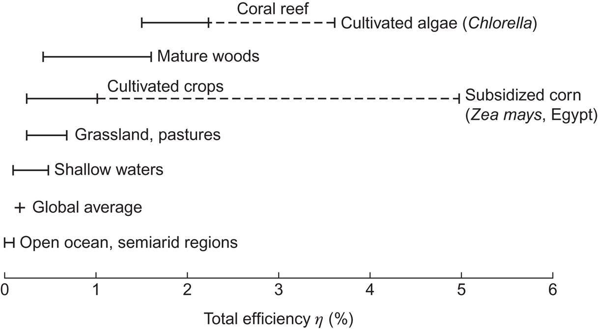
The range of efficiencies of natural plants goes from practically nothing to a little over 2%, the highest values being reached by tropical rain forests and algal cultures of coral reefs. Cultivated crops (terrestrial or marine) may reach 4–5% under optimal conditions and nutrient subsidy. The optimum efficiency from the theoretical discussion of equations (3.52) and (3.53) is roughly
(3.56)
Each of the conditions is difficult to achieve in practice, at least for extended periods. As mentioned earlier, mature ecosystems are characterized by diversity, which may not be reconcilable with maximum efficiency of primary production, and young ecosystems, such as non-perennial crops, need a growing period (cf. Fig. 3.96) before they reach full productivity, and thus their average efficiency on an area basis and over prolonged periods of time cannot be optimal.
Figure 3.99 gives a recent estimate of the geographical distribution of potential biomass production. The data are net primary production data derived from the Terrestrial Ecosystem Model (TEM) of the Woods Hole group (Melillo and Helfrich, 1998; Raich et al., 1991; Melillo et al., 1993; McGuire et al., 1997; Sellers et al., 1997). The assumption is that a mature ecosystem of natural vegetation has developed, and the model takes into account solar radiation, moisture, and temperature, as well as access to water and nutrients. Not included here is global warming (increased CO2), which could induce increased primary production in a fairly complex pattern and change the borders of natural vegetation zones, sometimes by several hundred kilometers (IPCC, 1996). Use of these biomass data for energy scenarios is illustrated in Chapter 6. Seasonal variations of actual biomass land coverage, as deduced from satellite-based sensors, are regularly posted on the Internet (NOAA, 1998).


Part I: Mini projects, discussion issues, and exercises
I.1
Find out what has happened since the year 2000 (see in Table 1.1) to the amounts of renewable energy used, based upon available statistical data, either globally or for your region or country.
I.2
Order the prices given in Chapter 1.1 according to the type of energy (heat, fuels for industry or transportation, electricity) and the type of customers (wholesale, retail). Try to find out what is happening to these prices today (e.g., using annually updated sources, such as OECD, IEA, or Danish Energy Agency data). Have the relative prices changed?
I.3
Sustainability is a word often used in political statements. Discuss the difference between renewability and sustainability in the energy field. Examples could be wind power (where you can dismount the turbines should you no longer need them) and reservoir-based hydropower (which entails irreversible modifications of large flooded areas). Furthermore, is the sustainability requirement to be used only on the supply side? One might propose sustainability on the demand side to mean that the demand in question could be satisfied for the entire world population (should they so desire) without the environmental side-effects usually included in the definition of sustainability. Is it sustainable to drive large BMW cars using renewable hydrogen? Is it sustainable to build glass houses as long as the cooling and ventilation system is powered by wind? Discuss the argument that, because there is a ceiling on each renewable energy flow, every proposed demand should be evaluated and ranked, with the possibility of disregarding perceived needs that turn out to be poorly ranked.
I.4
How could one design instruments for measurement of the individual components of the net radiation flux, e.g., direct, scattered, and reflected short-wavelength radiation, and upward- and downward-directed long-wavelength radiation? (This question is probably most interesting for those who are not acquainted with such instruments, and who might wish to compare their proposals with instruments actually in use, cf. Thekaekara, 1976; Robinson, 1966; Sellers, 1965; Meinel and Meinel, 1976.)
I.5
Discuss the formulation of approximate equations for the flow of water in rivers (cf., for example, Arnason, 1971).
I.6
Discuss the determinism of climate.
I.7
Discuss tides in the solid Earth and compare their properties with those in the oceans and those in the atmosphere. Construct, for instance, a simple model of a uniform interior of the Earth, a complete cover of ocean with fixed depth, and a uniform atmosphere of some effective height, and assume the densities for each of the three components to be constant (cf., for example, Tomaschek, 1957; Kertz, 1957).
I.8
Construct a simple one-dimensional model of the greenhouse effect, containing the Earth’s surface temperature Ts (variable), albedo as for short-wavelength radiation, and a′s for long-wavelength radiation; and an idealized atmosphere visualized as a layer (Fig. I.1) of uniform temperature Ta (variable), short-wavelength albedo aa, transmission coefficient ta, long-wavelength albedo a′a, and transmission coefficient t′a. Both the surface and the atmosphere emit long-wavelength radiation as blackbodies. All fluxes are treated as vertical.
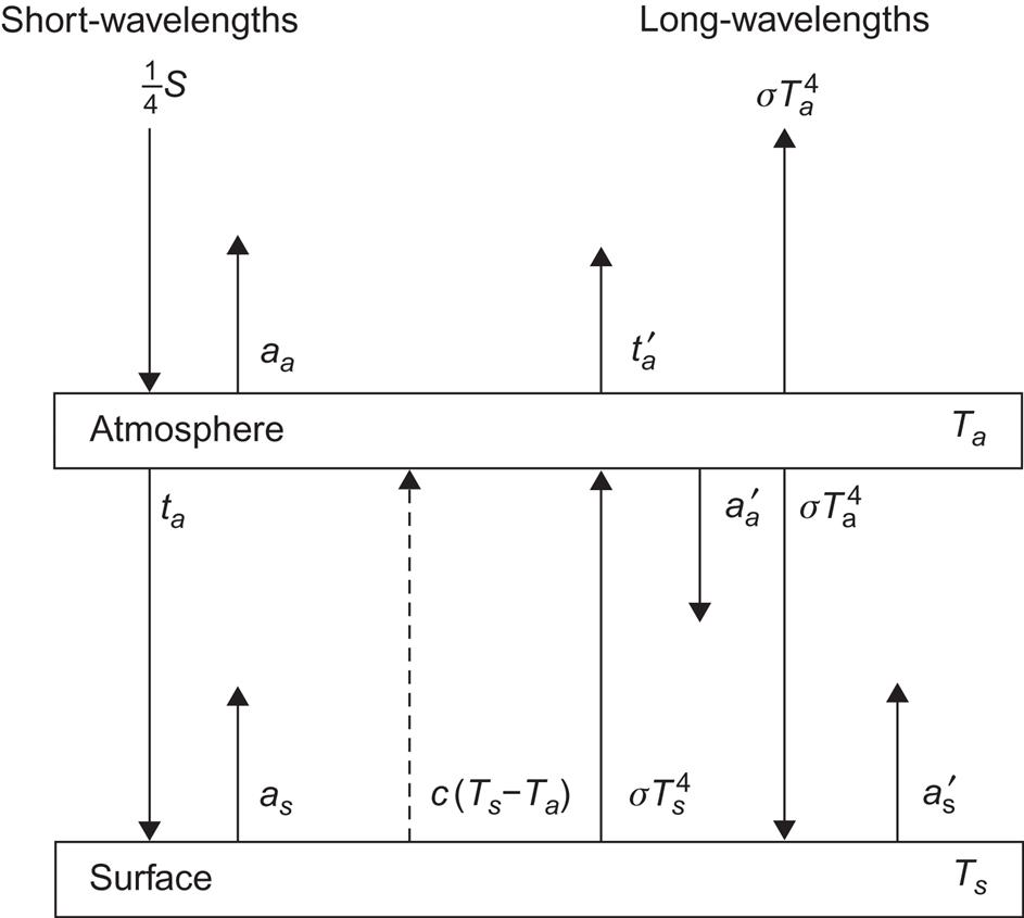
With a definite assumption regarding the non-radiative transfer between surface and atmosphere, such as assuming the flux to be proportional to (Ts – Ta), a set of parameters may be set up that reproduce the main features of the observed Earth–atmosphere system (cf. Fig. 2.20). Now questions can be asked concerning the sensitivity of the model to the parameters entering into it. How does the surface temperature change if aa is changed by ±10% (changing the albedo of the surface)? If the present energy use of human society were to be covered by solar collectors of average efficiency 0.2, and as was changed from 0.15 to zero for the area covered by these collectors, then how much would the total albedo as of the Earth’s surface become diminished? How does the surface temperature change if aa is changed by ±10% (e.g., due to presence of aerosols)? How does the surface temperature change if a′a is changed by ±10% (e.g., due to the presence of CO2)?
Although a computer-based model may offer the easiest approach to solving this problem, an approximate, analytical solution has been developed by Foong, S. (2006).
I.9
In connection with the failure to detect neutrinos from the Sun in the expected quantity, it has been suggested that energy production in the Sun’s core by nuclear processes (and therefore the neutrino flux) may be variable and that the present production may be in a valley. How would this affect radiation from the Sun’s surface? Would it be possible, by suitable choice of a periodic variation in solar energy production, to account for some of the climatic changes of the past? (See Ulrich, 1975.)
I.10
Discuss the reflected flux of solar radiation on an inclined plane, in front of which a horizontal mirror of given dimensions has been placed (cf., for example, Seitel, 1975).
I.11
What data on solar radiation, wind, waves, etc., are available in your region? (For example, check with the local meteorological service.)
I.12
Discuss the cooling of the Earth in terms of simplified models, such as: (a) a uniform sphere of constant heat capacity and diffusion coefficient, initially at a uniform temperature; (b) adding radiogenic heat production in the crust, by constraining the surface temperature to be the sum of two terms, one entirely due to the heat flow from the interior, and the other term exponentially decaying, such that the drop in 4.5×10⁹ years becomes 900 K.
Use present surface heat flow and temperature (average values) as boundary conditions, and discuss the long-range development of thermal conditions in the interior of the Earth (cf., for example, Goguel, 1976). Recent models suggest a core temperature of nearly 4000 K (Hofmeister, 1999).
I.13
Consider a compartment model for biological energy production and transfer within a closed ecosystem of the general form shown in Fig. 3.73. Assume, for instance, that the limiting factor governing the rate of primary production is solar radiation, so that the production becomes proportional to a schematic solar input, constant or with only seasonal sinusoidal variations [cf. (3.47)]. Think of a food chain in which you may find data on the rates and biomass levels appearing in Fig. 3.73 or some modification of it, and try to determine conditions for stability (no net production in the community as a whole).
If you have a computer at hand, you might try to set up a numerical simulation model for the system, assuming each rate (time derivative of a compartment level) to be a linear combination of all the compartment levels (some coefficients may be zero, of course). In this case you may also be able to follow the growth phase of the system, and attempt to judge whether the parameter values chosen are reasonable (cf., for example, Odum, 1972, where examples of parameter values may also be found; Patten, 1971–1972; Sørensen, 1975).
I.14
Use current biomass production data (available on the Internet) mentioned in connection with Fig. 3.79 to estimate possible bioenergy sources present in your region and their seasonal distribution. Does the seasonality have implications for energy use? Compare your results with the model considered in Chapter 6.