
Energy system planning
Abstract
This chapter describes planning methodology with the use of demand and supply scenarios, involving matching system construction supplemented with implementation pathway analysis. Human needs and desires are used to describe primary and secondary energy demands, and economic system efficiency optimization is invoked. Examples are provided on several levels. First, individual systems based on solar, wind, biofuel, and food production are considered. Simulations are performed with constraints of internal consistency, for local, regional, and global energy systems. Detailed scenario simulations are made for Europe, North America, and South-East Asia, where all regions are shown to allow a 100% renewable energy system.
Keywords
Scenario construction; Energy demand scenario; Energy supply scenario; Energy system simulation; Renewable energy scenario for USA; Renewable energy scenario for China; Renewable energy scenario for Japan; Renewable energy scenario for Mediterranean region
6.1 Methodology of energy planning
In Chapter 4, energy conversion devices are largely viewed as separate entities. In this chapter, they are regarded as parts of larger systems, which may comprise several converter units, storage facilities, and transmission networks. The determinant of each system is, of course, the purpose it is meant to serve, i.e., the end-point of the energy conversion processes. Therefore, a systems study must include analysis of both the end-uses (loads or demands) and the chains of conversion and transport steps connecting the primary energy source extraction with the loads, as well as spatial and temporal variations of supply and demand.
It is important to agree on the definition of end-use energy. There is the energy delivered to the end-user, and after subtraction of the losses in the final conversion taking place at the end-user, there is a net amount of energy being made useful. However, the real demand is always a product or a service, not the energy in itself. This implies that true energy demand is often difficult to pinpoint, because novel ways of satisfying the non-energy final need could radically change the end-use energy “required” or “demanded.” A typical definition used in practice is the lowest amount of energy associated with delivering the product or service demanded, as measured after the final conversion at the end-user and selected among all conversion schemes that can be realized with present knowledge. For some technologies, there will be a thermodynamic limit to energy conversion efficiency, but whether it is fundamental or may be circumvented by going to a different technology depends upon the nature of the final product or service. For many services, the theoretical minimum energy input is zero. Future advances in technology or new ideas for satisfying a particular need may change the minimum amount of end-use energy, and one should decide on which of the following to use in the definition:
• only technology available in the marketplace today, or
• only technology proven today and with a potential for market penetration, or
The outcome will be different, depending on the choice of technology level, and, in comparisons of system solutions, it is important to use the same definition of demand throughout. My preference is to use best technology available today in defining end-use, but any definition will do if it is used consistently.
6.1.1 Use of the scenario concept
This chapter gives examples of energy system simulations. Some of the examples simulate the function of existing systems, while others deal with hypothetical systems that may be created in the future. They will be analyzed using the scenario method, which is a way of checking the consistency of proposed energy systems as part of a view of the general future development of a society.
Scenario studies are meant to assist the decision-making process by describing a given energy system in its social context, in a way suitable for assessing systems not yet implemented. Simple forecasts of demand and supply based on economic modeling cannot directly achieve this, as economic theory deals only with the past and occasionally the present structure of society (cf. Chapter 7). To deal with the future, economic modelers may invoke the established quantitative relations between parts of the economic system and assume that they stay valid in the future. This produces a “business-as-usual” forecast. Because the relations between the ingredients of the economy, e.g., expressed through an input–output matrix, vary with time, one can improve the business-as-usual forecast by taking into account trends already present in past development. However, even trend forecasts cannot be expected to retain their validity for very long periods, and it is not just the period of forecasting time that matters, but also changes in the rules governing society. The rules may change due to abrupt changes in technology used (in contrast to the predictable, smooth improvements of technological capability or average rate of occurrence of novel technologies), or they may be changed by deliberate policy choices. It is sometimes argued that econometric methods could include such non-linear behavior by replacing the input–output coefficients with more complex functions. However, prediction of these functions cannot be based on studies of past or existing societies, because the whole point in human choice is that options are available that are different from past trends. The non-linear, non-predictable relations that may prevail in the future, given certain policy interventions at appropriate times, must therefore be postulated on normative grounds. This is what the scenario method does, and any attempt to mend economic theory also implies invoking a scenario construction and analysis, so, in any case, this is what has to be done (Sørensen, 2001).
It is important to stress that scenarios are not predictions. They should be presented as options that may come true if a prescribed number of actions are carried out. In democratic societies, this kind of change happens only if it is preceded by value changes that affect a sufficiently large portion of the society. Generally, in a democratic society, the more radically a scenario differs from present conditions, the larger the support it requires among the population. For non-democratic societies, where change may be implemented by decree, negative implications can easily entail.
The actual development may comprise a combination of some reference scenarios selected for analysis, with each reference scenario being a clear and perhaps extreme example of pursuit of a concrete line of political preference. It is important that the scenarios selected for political consideration be based on values and preferences that are important in the society in question. The value basis should be made explicit in the scenario construction. Although all analysis of long-term policy alternatives is effectively scenario analysis, particular studies may differ in their comprehensiveness of the treatment of future society. A simple analysis may make normative scenario assumptions only for the sector of society of direct interest in the study (e.g., the energy sector), assuming the rest to be governed by trend rules similar to those of the past. A more comprehensive scenario analysis will make a gross scenario for the development of society as a whole, as a reference framework for a deeper investigation of the sectors of particular interest. One may say that the simple scenario is one that uses trend extrapolation for all sectors of the economy except the one focused upon, whereas the more radical scenario will make normative, non-linear assumptions regarding the development of society as a whole. The full, normative construction of future societies will come into play for scenarios describing an ecologically sustainable global society, whereas scenarios aiming only at avoiding or coping with one particular problem, such as the climate change induced by greenhouse warming, are often of the simpler kind. Both types are exemplified in the scenario work described below.
6.1.2 Treatment of the time variable
In order to predict the performance of systems consisting of one or several energy converters, stores, and transmission devices, a mathematical model of the energy flow may be constructed. Such a model is composed of a number of energy conversion and transport equations, including source and sink terms corresponding to the renewable energy input and the output to load areas, both of which vary with time. The conversion processes depend on the nature of the individual devices, and the description of such devices (cf. Chapter 4) aims at providing the necessary formulae for a sufficiently complete description of the processes involved. In a number of cases (e.g., among those considered in Chapter 4), only a steady-state situation is studied, and the energy outputs are calculated for a given level of energy input. In a time-dependent situation, this type of calculation is insufficient, and a dynamic description must be introduced in order to evaluate the response time and energy flow delay across the converter (see, for example, section 4.3.6). Similar remarks apply to the description of storage systems, and, finally, the transmission network introduces a further time dependence and a certain delay in the energy flow reaching the load areas. The transmission network is often in the form of pipelines carrying a flow of some fluid (e.g., natural gas, hydrogen, or hot water) or an electric conductor carrying a flow of electric current. Additional transport of energy may take place in containers (e.g., oil products or methanol carried as ship, rail, or road cargo).
In order to arrive at manageable problems, it is, in most cases, necessary to simplify the time dependence for some parts of the system. First, short-term fluctuations in the source energy flow may, in some circumstances, be left out. This is certainly possible if the conversion device is itself insensitive to fluctuations of sufficiently high frequency. It could be so in a wind energy converter due to the inertia of the rotating mass, or, in a solar heat collector, due to the time constant for temperature changes in the absorber plate (and also in the circulating fluid). It may also be a valid approximation if short-term variations in the energy flux from the source can be regarded as random and if the collection system consists of a large number of separate units placed in such a way that no coherence in the fluctuating inputs can be expected.
Second, the performance of the conversion devices may often be adequately described in terms of a quasi-steady-state approximation. This consists of calculating an instantaneous energy output from the converter based on an instantaneous energy input as if the input flux were permanent, i.e., doing a steady-state calculation for each moment of time. This excludes an assessment of the possible time delay between the input flux and the output flux. If a solid mechanical connection transfers the energy through the converter (e.g., the rotor–shaft–gearbox–electric generator connections in a horizontal-axis wind energy converter), the neglect of time delays is a meaningful approximation. It may also be applicable for many cases of non-rigid transfer (e.g., by a fluid) if short-term correlations between the source flux and the load variations are not essential (which they seldom are in connection with renewable energy sources). For the same reason, time delays in transmission can often be neglected. The flow received at the load points may be delayed by seconds or even minutes, relative to the source flow, without affecting any of the relevant performance criteria of the system.
On the other hand, delays introduced by the presence of energy storage facilities in the system are essential features that cannot, and should not, be neglected. Thus, storage devices will have to be characterized by a time-dependent level of stored energy, and the input and output fluxes will, in general, not be identical. The amount of energy W(Si) accumulated in the storage Si can be determined from a differential equation of the form
(6.1)
or from the corresponding integral equation. The individual terms in the two expressions involving summation on the right-hand side of (6.1) represent energy fluxes from the converters to and from the storage devices. The loss term ![]() may depend on the ingoing and outgoing fluxes and on the absolute amount of energy stored in the storage in question, W(Si).
may depend on the ingoing and outgoing fluxes and on the absolute amount of energy stored in the storage in question, W(Si).
In practice, the simulation is performed by calculating all relevant quantities for discrete values of the time variable and determining the storage energy contents by replacing the time integral of (6.1) by a summation over the discrete time points considered. This procedure fits well with the quasi-steady-state approximation, which at each integration step allows the calculation of the converter outputs (some of which are serving as storage inputs ![]() ) for given renewable energy inputs, and similarly allows the calculation of conversion processes in connection with the storage facilities, and the energy fluxes
) for given renewable energy inputs, and similarly allows the calculation of conversion processes in connection with the storage facilities, and the energy fluxes ![]() to be extracted from the storage devices in order to satisfy the demands at the load areas. If the time required for conversion and transmission is neglected, a closed calculation can be made for each time integration step. Interdependence of storage inputs and outputs, and of the primary conversion on the system variables in general (e.g., the dependence of collector performance on storage temperature for a flat-plate solar collector), may lead to quite complex calculations at each time step, such as the solution of non-linear equations by iteration procedures (section 4.4.3).
to be extracted from the storage devices in order to satisfy the demands at the load areas. If the time required for conversion and transmission is neglected, a closed calculation can be made for each time integration step. Interdependence of storage inputs and outputs, and of the primary conversion on the system variables in general (e.g., the dependence of collector performance on storage temperature for a flat-plate solar collector), may lead to quite complex calculations at each time step, such as the solution of non-linear equations by iteration procedures (section 4.4.3).
If finite transmission times cannot be neglected, they may be included, to a first approximation, by introducing simple, constant delays, such that the evaluations at the mth time step depend on the values of certain system variables at earlier time steps, m–d, where d is the delay in units of time steps. The time steps need not be of equal length, but may be successively optimized to obtain the desired accuracy with a minimum number of time steps by standard mathematical methods (see, for example, Patten, 1971, 1972).
The aim of modeling may be to optimize either performance or system layout. In the first case, the system components are assumed to be fixed, and the optimization aims at finding the best control strategy, i.e., determining how best to use the system at hand (“dispatch optimization”). In a multi-input–multi-output conversion system, this involves choosing which of several converters to use to satisfy each load and adjusting inputs to converters in those cases where this is possible (e.g., biofuels and reservoir-based hydro as opposed to wind and solar radiation). For system optimization, the structure of the conversion system may also be changed, with recognition of time delays in implementing changes, and the performance over an extended period would be the subject of optimization. For simple systems (without multiple inputs or outputs from devices), linear programming can furnish a guaranteed optimum dispatch of existing units, but, in the general case, it is not possible to prove the existence of an optimum. Still, there are systematic ways to approach the optimization problem, e.g., by using the method of steepest descent for finding the lowest minimum of a complex function, combined with some scheme for avoiding shallow, secondary minima of the function to minimize (Sørensen, 1996, 1999).
6.2 Demand scenario construction
The demand for products or services using energy, taken at the end-user after any final conversion done there, is basically determined by the structure of society, the technology available to it, and the activities going on within it—and, behind these, the aims, desires, and habits of the people constituting the society in question.
Enumerating the energy demands coming out of such appraisals can be done methodologically, as in section 6.2.3, but first it may be illustrative to paint a broad picture of possible developments of societies, as they pertain to energy end-use demand and to the intermediary energy demands of energy conversion processes made necessary by the structure of the energy system (Sørensen, 2008b). Both of these are sketched below for a limited range of development scenarios, without claiming completeness and clearly basing the construction on normative positions. The end-use scenarios are called precursor scenarios, to distinguish them from the actual scenarios created later that specify the energy use quantitatively. The corresponding scenarios for intermediary conversion system scenarios are usually characterized by their emphasis on efficiency. Of course, the overall structure of the energy system can be fixed only after both end-use demands and the supply options to be exploited have been decided, and the intersociety (whether regions within a country or international) setting (trade, grid connections, etc.) is known.
6.2.1 End-use precursor scenarios
6.2.1.1 Runaway precursor scenario
In the runaway scenario, the energy demand grows at least as quickly as the overall economic activity (measured, for example, by the gross national product). This has historically been the case during periods of exceptionally low energy prices, notably in the years around 1960. Conditions for this scenario, in addition to low energy prices, include: in the transportation sector increased passenger-kilometers (facilitated by more roads, cheap air connections, and decentralization of the locations of homes, workplaces, and leisure facilities) and increased ton-kilometers of freight haul, both locally and globally (facilitated by decentralization of component production and inexpensive worldwide shipment of parts and products); in the building sector, more square meters of living space and more square meters per unit of economic activity; and, in the electricity sector, more appliances and other equipment. Building-style developments could create a perceived need for air conditioning and space cooling. For industry, there could be increased emphasis on energy-intensive production in countries with low labor costs, and the opposite in countries with high labor costs. However, service-sector activities and their energy use could increase substantially, with greatly enlarged retail shopping areas and use of much more light and other energy-demanding displays for business promotion. For leisure activities, traditional nature walks or swimming could be replaced by motocross, speedboat use, and other energy-demanding activities.
6.2.1.2 High-energy-growth precursor scenario
The high-energy-growth scenario is similar to the runaway scenario, but with a slower, but still significant, increase in energy demand. In the transportation sector, this could be due to a certain saturation tendency in transport activities, caused by the higher value placed on time lost in traveling on more congested roads and in more congested air space. For industry, continued decrease in energy-intensive production may lead to demand growing more slowly than the economic activity. In buildings, heat use may increase less than floor area, due to zoning practices, etc. Generally, activity level and energy demand may undergo a certain amount of decoupling, reflecting the fact that the primary demands of a society are goods and services, and that these can be provided in different ways with different energy implications. An effect of this type damps the energy demand in the high-energy-growth scenario, as compared to the runaway scenario, but due more to technological advances and altered industry mix than to a dedicated policy aimed at reducing energy demand.
6.2.1.3 Stability precursor scenario
The stability scenario assumes that end-use energy demand stays constant, despite rearrangements in specific areas. Specifically, in the building sector, energy demand is assumed to saturate (that is, the number of square meters per person occupying the building, whether for work or living, will not continue to increase, but reach a natural limit with enough space for the activities taking place, without excessive areas to clean and otherwise maintain). In the industrial sector, increasingly knowledge-based activity will reduce the need for energy-intensive equipment, replacing it primarily by microprocessor-based equipment suited for light and flexible production. Industrial energy use will decline, although industries in the service and private sectors will continue to add new electronic equipment and computerized gadgets. In other sectors, dedicated electricity demand will increase substantially, but, in absolute terms, it will be more or less compensated for by the reductions in the industrial sector. For transportation, saturation is assumed both in number of vehicles and number of passenger- or ton-kilometers demanded, for the reasons outlined above in the section on the high energy-growth scenario. Explanations for this could include the replacement of conference and other business travel by video conferencing, so that an increase in leisure trips may still be possible. Presumably, there have to be transportation-related strategies implemented for this to be realistic, including abandoning tax rebates for commercially used vehicles and for business travel, and possibly also efforts in city planning to avoid the current trend toward increased travel distances for everyday shopping and service delivery. The stability scenario was used as the only energy demand scenario in some earlier studies on the possibilities for hydrogen use in the Danish energy system (see Sørensen et al., 2001, 2004; Sørensen, 2005).
6.2.1.4 Low-energy-demand precursor scenario
In the low-energy-demand scenario, full consideration is paid to the restructuring of industry in countries making a transition from a goods orientation to service provision. Today, many enterprises in Europe or the United States already only develop new technology (and sometimes test it on a limited domestic market): once the technology is ready for extended markets, production is transferred to low-wage companies, currently in Southeast Asia. This change in profit-earning activities has implications for the working conditions of employees. Much of the information-related work can be performed from home offices, using computer equipment and electronic communications technology, and thereby greatly reducing the demand for physical transportation.
In the retail food and goods sector, most transactions between commerce and customer will be made electronically, as is already the case in a number of subsectors today. An essential addition to this type of trade is the market for everyday products, where, before, customers made limited use of electronic media to purchase grocery and food products, probably because of their perceived need to handle the goods (for example, to examine fruit to see if it is ripe) before purchasing them. Clearly, better electronic trade arrangements, with video inspection of actual products, could change customers’ practices. If everyday goods are traded electronically, their distribution will also be changed toward an optimal dispatch that requires considerably less transport energy than current shopping practices do. Overall, a substantial reduction in energy demand will result from these changes, should they come true. In the remaining manufacturing countries, these changes are expected to take place equally fast, if not faster, due to workers’ less-flexible time schedules for shopping. Thus, economic development is further decoupled from energy use and may continue to exhibit substantial growth.
6.2.1.5 Catastrophe precursor scenario
In the catastrophe scenario, reduced energy demand is due to failure to achieve desirable economic growth. Reasons could be the over-allocation of funds to the financial sector, causing major periodic economic recessions. In some European and North American countries, additional reasons could include the current declining public and political interest in education, particularly in those areas most relevant to a future knowledge society. In this scenario, there would be a decreased number of people trained in skills necessary for participating in international industrial and service developments, and the opportunity to import people with these intellectual skills would have been lost by the imposition of immigration policy unfavorable to precisely the regions of the world producing a surplus of people with technical and related creative high-level education.
Although there are pessimists who view this scenario as the default if there is no immediate change in the political climate in the regions with such problems, the stance here is that the traditional openness of many Western societies will work to overcome the influence of certain negative elements. This is particularly true for small countries like Denmark, if it can maintain a distance from globalization pressures from the European Union, the U.S.-dominated World Trade Organization, etc. Even if Denmark should choose to continue to concentrate on less education-demanding areas, such as coordination and planning jobs in the international arena (which require primarily language and overview skills), these could easily provide enough wealth to a small nation of open-minded individuals willing to serve as small wheels in larger international projects. The current economic decline would become a passing crisis, to be followed by a niche role for Denmark, which in energy terms would imply returning to one of the central scenarios described above. Only if Denmark became internationally isolated would this option fade away and the catastrophe scenario become a reality.
This discussion uses Denmark, a small country, as an example. In other countries, some aspects of these same problems are also evident, and if a country that lowers skills through poor information policies (e.g., in news media) and bad consumer choices (influenced by the curricula offered by schools and universities) is large, then a downturn may be more difficult to avoid.
6.2.2 Intermediary system efficiency
Many countries, particularly in Europe, have a long tradition of placing emphasis on efficient conversion of energy. Following the 1973/4 energy crises, detached homes (where the occupants are also the owners making decisions on investments) in particular were retrofitted to such an extent that overall low-temperature heat use dropped by almost a third over a decade. Carbon-emission and pollution taxes on electricity and transportation fuels (taxes that are not always clearly labeled) have influenced the mix of appliances being installed and car models bought, with the lowest-energy-consuming equipment dominating the market in some countries. This trend is only partial, because there are still substantial sales of luxury cars and 4-wheel-drive special utility vehicles not serving any apparent purpose in countries with hardly any unpaved roads. Transmission losses are fairly low in Europe, where underground coaxial cables have been installed, mainly to avoid the vulnerability of overhead lines during storms.
Following are three precursor-scenario outlines illustrating the planning considerations made implicitly or explicitly by planners and legislators.
6.2.2.1 Laisser-faire precursor scenario
In the laisser-faire scenario, conversion efficiencies are left to the component and system manufacturers, which would typically be international enterprises (such as vehicle and appliance manufacturers, power station and transmission contractors, and the building industry). The implication is that efficiency trends follow an international common denominator, which at least in the past has meant lower average efficiency than suggested by actual technical advances and sometimes even lower than the economic optimum at prevailing energy prices. Still, efficiency does increase with time, although often for reasons not related to energy (for example, computer energy use has been lowered dramatically in recent years, due to the need to avoid component damage by excess heat from high-performance processors). The gross inadequacies of the current system, deriving from tax-exemption of international travel and shipping by sea or air, and its impact on choice of transportation technology, are assumed to prevail.
6.2.2.2 Rational investment precursor scenario
In the rational investment scenario, the selection of how many available efficiency measures will actually be implemented, through the technologies chosen at each stage in the time development of the energy system, is based on a lifetime economic assessment. This means that the efficiency level is not chosen according to a balancing of the cost of improving efficiency with the current cost of energy used by the equipment, but with the present value of all energy costs incurred during the lifetime of the equipment. This assessment requires an assumption of future average energy costs and it is possible, by choice of the cost profile, to build in a certain level of insurance against unexpected high energy prices. The important feature of the rational investment scenario is that it forces society to adopt a policy of economic optimization in the choice of energy-consuming equipment and processes. This policy is partially implemented at present, e.g., through energy provisions in building codes, through appliance labeling, and through vehicle taxation. In the last case, there is a distinction between the efficiency optimization for a vehicle with given size and performance, considered here, and the question of proper vehicle size and performance characteristics dealt with in the previous section on end-use energy. The energy taxation currently used in many countries for passenger cars does not make such a distinction, and the tax reduction for commercially used vehicles actually counters rational economic considerations; it should be characterized as taxpayers’ subsidies for industry and commerce.
6.2.2.3 Maximum-efficiency precursor scenario
One version of the maximum-efficiency scenario could require that every introduction of new energy-consuming equipment should use the best currently available technical efficiency. This implies selection of the highest-efficiency solution available in the marketplace, or even technology ready for, but not yet introduced into, the commercial market. Higher-efficiency equipment under development and not fully proven would, however, not be implemented, except as part of demonstration programs. This “best-current-technology” approach was used in several previous scenario studies (Sørensen, 1999, 2012; Sørensen and Meibom, 2000; Sørensen et al., 2001, 2004, and for some of the scenarios later in this chapter) with the rationale that current most-efficient technology can serve as a good proxy for average-efficiency technology 50 years in the future. Depending on assumptions regarding future energy prices, the rational investment precursor scenario could be less efficient, of similar efficiency, or of higher efficiency than the “best-current-equipment” approach.
Therefore, a more appropriate definition of the maximum-efficiency scenario would be based on projecting typical average efficiency improvements over the entire planning period, and then insisting that the best technology at each instant in time is used for all new equipment introduced at that moment in time. While projections of future efficiency of individual pieces of equipment may be uncertain and sometimes wrong, it seems reasonable to assume that average efficiencies over groups of related equipment can be extrapolated reliably.
6.2.3 Load structure
Loads are end-use energy demands as experienced by the energy system. From the consumer’s perspective, loads satisfy needs by delivering goods and services that require energy. Energy delivery is often constrained to certain time profiles and locations. This is the reason that energy systems often contain energy storage facilities, as well as import-export options, whether for transport by a grid or by vessels or vehicles. Some energy storage could be at the end-user and form part of the equipment used to satisfy the end-user’s demand (e.g., solar thermal systems with hot water tanks). Utilization of energy stores can modify both time variations and total amounts of energy demanded.
On a regional or national level, loads are customarily divided onto sectors, such as energy demands of industry, agriculture, commerce, services and residences, and transportation. A sector may require one or more types of energy, e.g., heat, electricity, or a “portable source” capable of producing mechanical work (typically a fuel). The distribution of loads on individual sectors depends on the organization of the society and on climatic conditions. The latter influence the need for space heating or cooling, while the former includes settlement patterns (which influence the need for transportation), building practices, health care and social service levels, types of industry, etc. A systematic method of treating energy demands is described in the following, for use in the scenarios and system simulations in sections 6.5–6.7.
The development of energy demands is sometimes discussed in terms of marginal changes relative to current patterns. For changes over extended periods of time, this is not likely to capture the important issues. Another approach, called the bottom-up model, looks at human needs, desires, and goals and then builds up, first, the corresponding material demands requirement and then the energy required to fulfill these demands, under certain technology assumptions (Kuemmel et al., 1997, appendix A). This approach is based on the view that certain human needs are basic needs, i.e., non-negotiable, while others are secondary needs that depend on cultural factors and stages of development and knowledge and could turn out differently for different societies, subgroups, or individuals within a society. Basic needs include adequate food, shelter, security, and human relations. Then there is a continuous transition to more negotiable needs, which include material possessions, art, culture, human interactions, and leisure. [Maslow (1943) was among the first to discuss the hierarchy of human needs.] Energy demand is associated with satisfying several of these needs, with manufacture and construction of the equipment and products used in fulfillment of the needs, and with procuring the materials needed along the chain of activities and products.
In normative models like scenarios for the future, the natural approach to energy demand is to translate needs and goal satisfaction into energy requirements, consistent with environmental sustainability in case that is part of the normative assumptions. For market-driven scenarios, basic needs and human goals play an equally important role, but secondary goals are more likely to be influenced by commercial interest rather than by personal motives. It is interesting that the basic needs approach is routinely taken in discussion of the development of societies with low economic activity, but rarely in discussions of industrialized countries.
The methodology developed here is first to identify needs and demands (in short, human goals), and then to discuss the energy required to satisfy them in a series of steps tracing backward from the goal-satisfying activity or product to any required manufacture and then further back to materials. The outcomes are expressed on a per capita basis (involving averaging over differences within a population), but separates different geographical and social settings as required for local, regional, or global scenarios.
Analysis may begin by assuming 100% goal satisfaction, from which energy demands in societies that have not reached this level can subsequently be determined. Of course, a normative scenario may include the possibility that some members of the society do not enjoy full goal satisfaction. This is true for liberalism, which considers inequality a basic economic driver in society. Nevertheless, the end-use approach assumes that it is meaningful to specify the energy expenditure at the end-user without considering the system responsible for delivering the energy. This is only approximately true. In reality, there may be couplings between the supply system and the final energy use, and therefore in some cases end-use energy demand is dependent on the overall system choice. For example, a society rich in resources may undertake production of large quantities of resource-intensive products for export, while a society with fewer resources may instead focus on knowledge-based production; both societies are interested in balancing their economy to provide satisfaction of the goals of their populations, but possibly with quite different implications for energy demand.
End-use energy demands are distributed both on usage sectors and on energy qualities, and they may be categorized as follows:
1. Cooling and refrigeration 0°C–50°C below ambient temperature
2. Space heating and hot water 0°C–50°C above ambient temperature
4. Process heat in the range 100°C–500°C
6. Stationary mechanical energy
7. Electric energy (no simple substitution possible)
The goal categories used to describe the basic and derived needs can then be selected as follows:
A: Biologically acceptable surroundings
f4: Raw materials and energy industry
Here categories A–E refer to direct goal satisfaction, f1–f4 to primary derived requirements for fulfilling needs, and, finally, f5–f7 to indirect requirements for carrying out the various manipulations stipulated. Ranges of estimated energy requirements for satisfying all needs identified by present societies are summarized in Table 6.1 (Kuemmel et al., 1997), with a more detailed, regional distribution given in Table 6.2 for a 2050 scenario-study by Sørensen and Meibom (1998). The same study includes an analysis of year-1994 energy end-uses, using the same principles as for the future scenario, and this analysis is given in Table 6.3. The table shows the low average efficiencies of the final conversion steps in 1994. The detailed assumptions behind the “full goal satisfaction” energy estimates are given below.
Table 6.1
Global end-use energy demand based upon bottom-up analysis of needs and goal satisfaction in different parts of the world, using best available currently available technologies (average energy flow in W cap−1)
| 1. Cooling & refrigeration | 2. Space heating | 3. Process heat under 100°C | 4. Process heat 100–500°C | 5. Process heat over 500°C | 6. Stationary mechanical energy | 7. Electric appliances | 8. Transportation work | 9. Food energy | TOTAL | |
| A. Biologically acceptable surroundings | 0–200 | 0–650 | 0 | 0 | 0 | 0 | 0 | 0 | 0 | 0–650 |
| B. Food and water | 21 | 0 | 5 | 7 | 0 | 0 | 0 | 0 | 120 | 153 |
| C. Security | (0) | (0) | 0 | 0 | 0 | (0) | 0 | 1 | 0 | 1 |
| D. Health | 0 | 0 | 115 | 17 | 0 | 0 | (0) | (0) | 0 | 132 |
| E. Relations, leisure | (0) | (0) | 0 | 0 | 0 | 0 | 60–82 | 25–133 | 0 | 85–215 |
| F. Activities: | ||||||||||
| Construction | 0 | 0 | 0 | 0 | 0 | 30–60 | 0 | 7–15 | 0 | 37–75 |
| Trade, service and distribution | 1–80 | 0–150 | 0–10 | 0 | 0 | 5 | 20 | 30–100 | 0 | 56–325 |
| Agriculture | 0 | 00 | 0 | 0–6 | 0 | 1–3 | 1 | 3–6 | 0 | 5–16 |
| Manufacturing industry | 1–40 | 0–150 | 10–100 | 20–70 | 12–30 | 20–40 | 20–40 | 7–15 | 0 | 90–445 |
| Raw Materials and energy industry | 0 | 0 | 0–30 | 0–30 | 0–250 | 0–170 | 0–30 | 0–20 | 0 | 0–530 |
| Education | 0–20 | 0–65 | 0 | 0 | 0 | 0 | 1–2 | 0 | 0 | 1–67 |
| Commuting | 0 | 0 | 0 | 0 | 0 | 0 | 0 | 0 | 0 | 0–30 |
| Total | 23–361 | 0–1015 | 130–260 | 44–130 | 12–280 | 56–278 | 102–175 | 73–320 | 120 | 560–2639 |
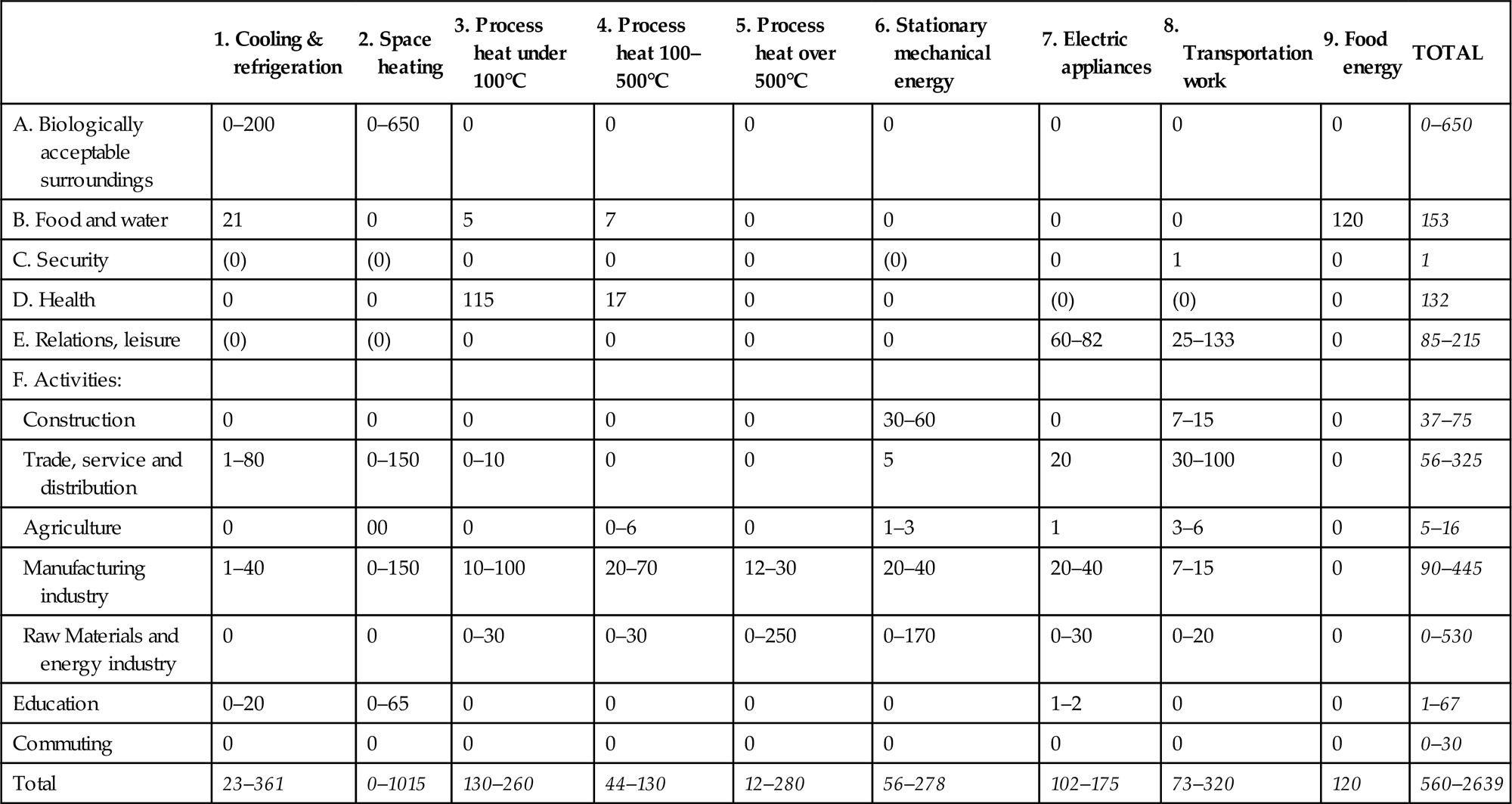
From Kuemmel et al. (1997).
Table 6.2
Per capita energy use for “full goal satisfaction” in W cap−1 and total in GW for the assumed 2050 population stated
| Regions &/Energy Quality: | 1. USA, Canada | 2. Western Europe, Japan, Australia | 3. Eastern Europe, Ex-Soviet, Middle East | 4. Latin America, SE Asian “tigers” | 5. China, India, Rest of Asia | 6. Africa | Average & Total |
| Space heating* | 205 | 212 | 164 | 19 | 96 | 10 | |
| Other low-temp. heat | 150 | 150 | 150 | 150 | 150 | 150 | |
| Medium-temp. heat | 50 | 50 | 50 | 50 | 50 | 50 | |
| High-temp. heat | 40 | 40 | 40 | 40 | 40 | 40 | |
| Space cooling* | 9 | 2 | 43 | 37 | 71 | 44 | |
| Other refrigeration | 35 | 35 | 35 | 35 | 35 | 35 | |
| Stationary mechanical | 150 | 150 | 150 | 150 | 150 | 150 | |
| Electric appliances | 150 | 150 | 150 | 150 | 150 | 150 | |
| Transportation | 200 | 150 | 200 | 150 | 150 | 150 | |
| Food energy | 120 | 120 | 120 | 120 | 120 | 120 | |
| Total 2050 end-use energy | 1109 | 1059 | 1102 | 901 | 1012 | 899 | 986 W/cap |
| 420 | 559 | 1146 | 1243 | 4008 | 1834 | 9210 GW | |
| Population 2050, mill. | 379 | 528 | 1040 | 1380 | 3960 | 2040 | 9340 |
| Total area, million km2 | 20.1 | 15.4 | 28.3 | 26.3 | 20.1 | 30.9 | 141.1 |
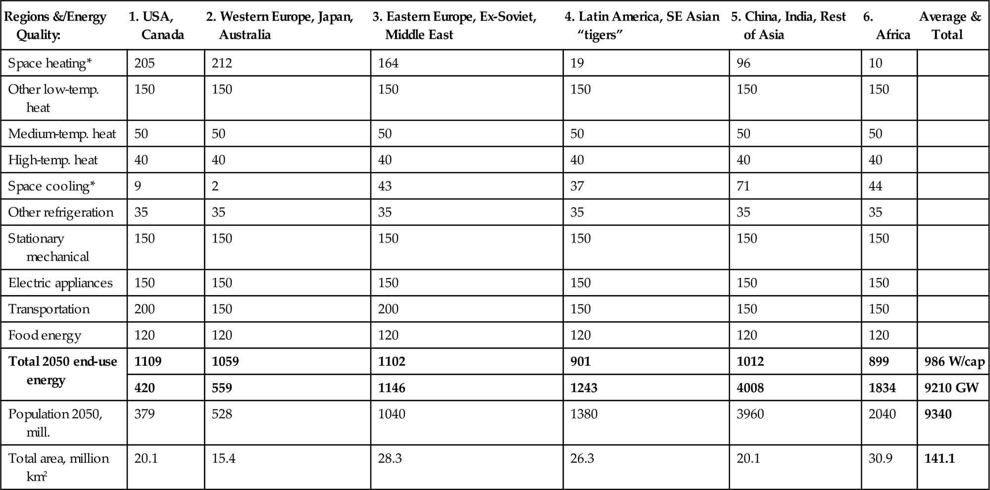
Rows marked * are based on temperature data for each cell of geographical area (0.5° longitude-latitude grid used). Manufacturing and raw materials industries are assumed to be distributed in proportion to population between regions. A full list of the countries included in each region is given in Sørensen and Meibom (1998).
Reprinted from Sørensen and Meibom (1998), with permission.
Table 6.3
Estimated end-use energy in 1994.
| Region: 1994 End-use Energy | 1. USA, Canada | 2. Western Europe, Japan, Australia | 3. Eastern Europe, Ex-Soviet, Middle East | 4. Latin America, SE Asian “tigers” | 5. China, India, Rest of Asia | 6. Africa | Average & Total |
| Space heating | 186 | 207 | 61 | 2 | 19 | 1 | 46 W/cap |
| 52 | 116 | 41 | 1 | 48 | 1 | 260 GW | |
| Other low-temp. heat | 120 | 130 | 40 | 15 | 18 | 10 | 36 W/cap |
| 34 | 73 | 27 | 12 | 47 | 7 | 199 GW | |
| Medium-temp. heat | 40 | 50 | 30 | 10 | 10 | 5 | 17 W/cap |
| 11 | 28 | 20 | 8 | 26 | 3 | 97 GW | |
| High-temp. heat | 35 | 40 | 30 | 10 | 10 | 3 | 16 W/cap |
| 10 | 22 | 20 | 8 | 26 | 2 | 88 GW | |
| Space cooling | 9 | 1 | 13 | 2 | 3 | 0 | 4 W/cap |
| 2 | 1 | 9 | 2 | 8 | 0 | 22 GW | |
| Other refrigeration | 29 | 23 | 14 | 2 | 2 | 0 | 7 W/cap |
| 8 | 13 | 9 | 1 | 5 | 0 | 37 GW | |
| Stationary mechanical | 100 | 130 | 80 | 25 | 5 | 4 | 34 W/cap |
| 28 | 73 | 53 | 21 | 13 | 3 | 191 GW | |
| Electric appliance | 110 | 120 | 50 | 20 | 5 | 4 | 29 W/cap |
| 31 | 67 | 33 | 16 | 13 | 3 | 164 GW | |
| Transportation | 200 | 140 | 40 | 20 | 5 | 3 | 34 W/cap |
| 56 | 79 | 27 | 16 | 13 | 2 | 193 GW | |
| Food energy | 120 | 120 | 90 | 90 | 90 | 90 | 95 W/cap |
| 34 | 67 | 60 | 74 | 233 | 61 | 530 GW | |
| Total end-use energy | 948 | 962 | 448 | 195 | 167 | 121 | 318 W/cap |
| 268 | 540 | 298 | 160 | 432 | 83 | 1781 GW | |
| Population 1994 | 282 | 561 | 666 | 820 | 2594 | 682 | 5605 million |
| Region area | 20 | 15 | 28 | 26 | 20 | 31 | 141 million km2 |

Due to the nature of available statistical data, the categories are not identical to those used in the scenarios. Furthermore, some end-use energies are extrapolated from case studies. These procedures aim to provide a more realistic scenario starting point. However, as the scenario assumptions are based upon basic principles of goal satisfaction, the inaccuracy of current data and thus of scenario starting points does not influence scenario reliability, but only stated differences between now and the future.
Reprinted from Sørensen and Meibom (1998), with permission.
For use in the year-2050 global scenario described in section 6.7, the end-use energy components for each category are estimated on the basis of the actually assumed partial goal fulfillment by the year 2050 and are given in Table 6.4 on a regional basis. This analysis assumes population development based on the United Nations population studies (United Nations, 1996), using the alternative corresponding to high economic growth (in the absence of which population is estimated to grow more). The population development is in good agreement with the central choice used in the energy emission scenarios created for the IPCC process (IPCC, 2007a-c).
Table 6.4
The fraction of “full goal satisfaction” assumed in the year-2050 scenario, with estimated values for 1994 given in parentheses.
| Regions: / Energy Quality: | 1. USA, Canada | 2. Western Europe, Japan, Australia | 3. Eastern Europe, Ex-Soviet, Middle East | 4. Latin America, SE Asian “tigers” | 5. China, India, Rest of Asia | 6. Africa |
| Space heating | 0.9 (0.9) | 1.0 (0.96) | 0.75 (0.25) | 0.67 (0.08) | 0.63 (0.16) | 0.15 (0.10) |
| Other low-temp. heat | 0.87 (0.8) | 1.0 (0.87) | 0.53 (0.27) | 0.6 (0.10) | 0.67 (0.12) | 0.13 (0.07) |
| Medium-temp. heat | 0.9 (0.8) | 1.0 (1.0) | 0.8 (0.6) | 0.8 (0.2) | 0.8 (0.2) | 0.1 (0.1) |
| High-temp. heat | 0.88 (0.88) | 1.0 (1.0) | 0.75 (0.75) | 0.75 (0.25) | 0.75 (0.25) | 0.13 (0.08) |
| Refrigeration | 1.0 (0.83) | 1.0 (0.67) | 0.4 (0.4) | 0.5 (0.05) | 0.33 (0.05) | 0.05 (0.01) |
| Stationary mechanical | 0.93 (0.67) | 1.0 (0.87) | 0.53 (0.53) | 0.67 (0.17) | 0.67 (0.03) | 0.13 (0.03) |
| Electric appliances | 1.0 (0.73) | 1.0 (0.8) | 0.53 (0.33) | 0.67 (0.13) | 0.67 (0.03) | 0.1 (0.03) |
| Transportation | 0.9 (1.0) | 1.0 (0.93) | 0.35 (0.20) | 0.67 (0.13) | 0.33 (0.03) | 0.1 (0.02) |
| Food energy | 1.0 (1.0) | 1.0 (1.0) | 1.0 (0.75) | 1.0 (0.75) | 1.0 (0.75) | 0.83 (0.75) |
| Averages of the above | 0.93 (0.85) | 1.0 (0.90) | 0.62 (0.45) | 0.68 (0.21) | 0.64 (0.18) | 0.20 (0.13) |
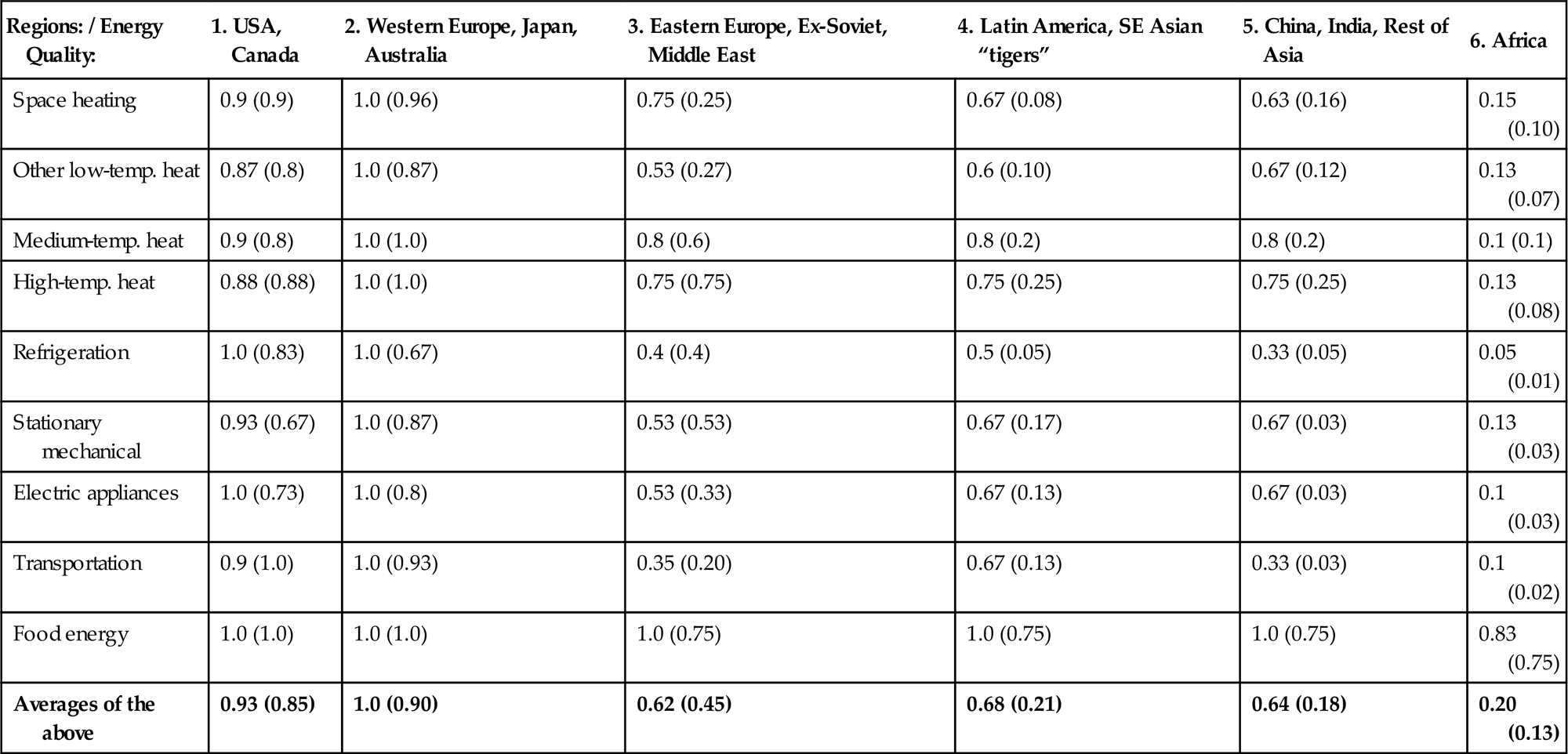
These estimates involve assumptions about conditions for development in different parts of the world: on the one hand, positive conditions, such as previous emphasis on education, which are a prerequisite for economic development, and, on the other hand, negative conditions, such as social instability, frequent wars, corrupt regimes, lack of tradition for democracy, for honoring human rights, and so on. It is recognized that these assumptions are considerably subjective. As an example, United Nations projections traditionally disregard non-economic factors and, for instance, assume a much higher rate of development for African countries.
Reprinted from Sørensen and Meibom (1998), with permission.
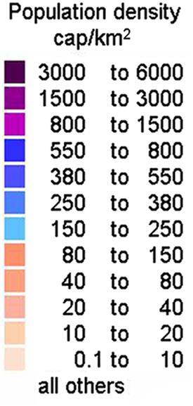
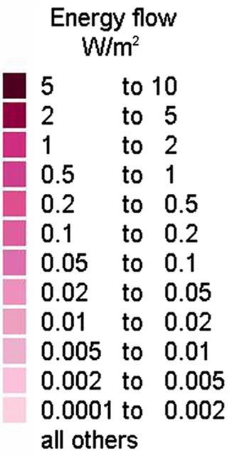
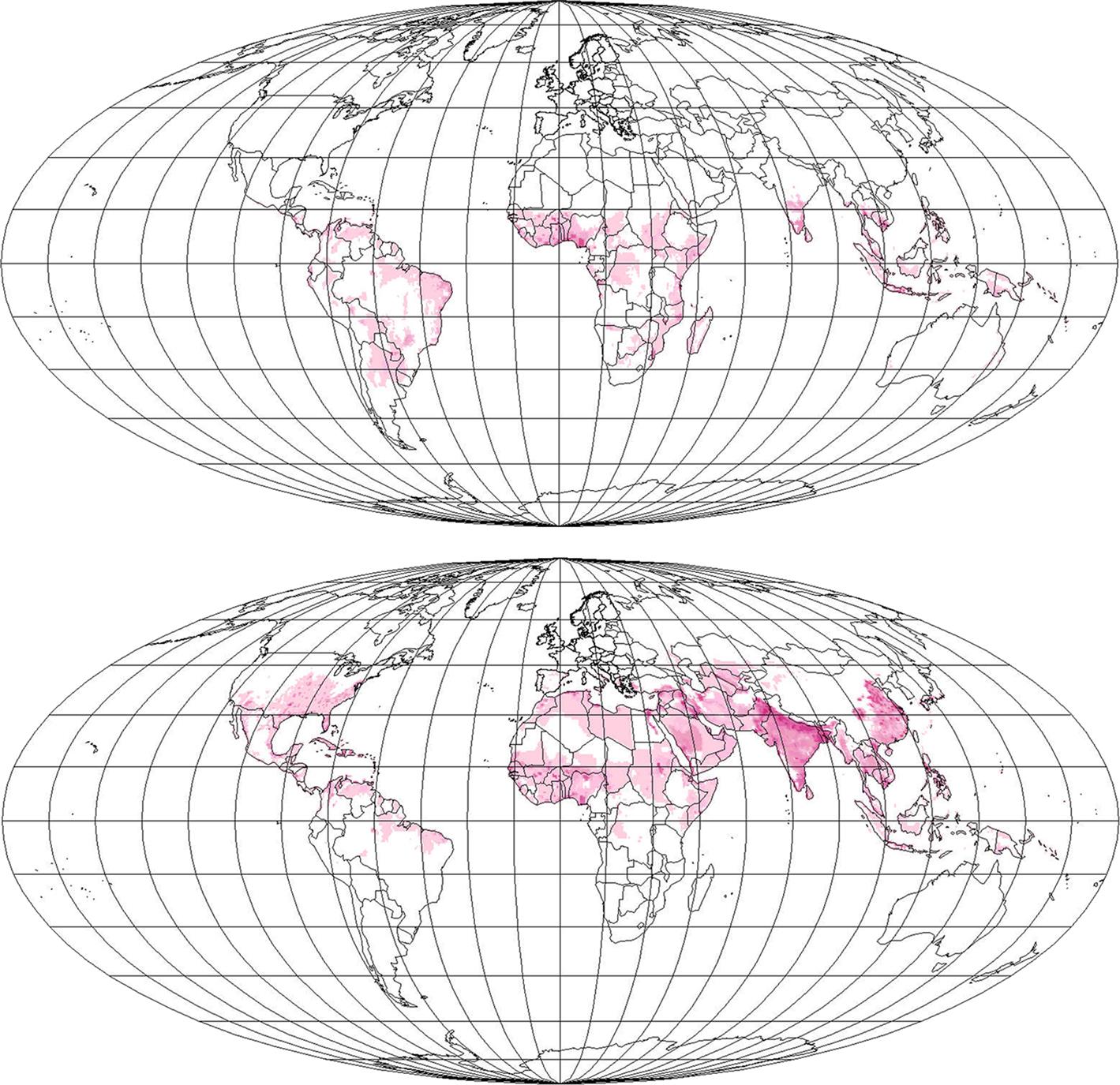
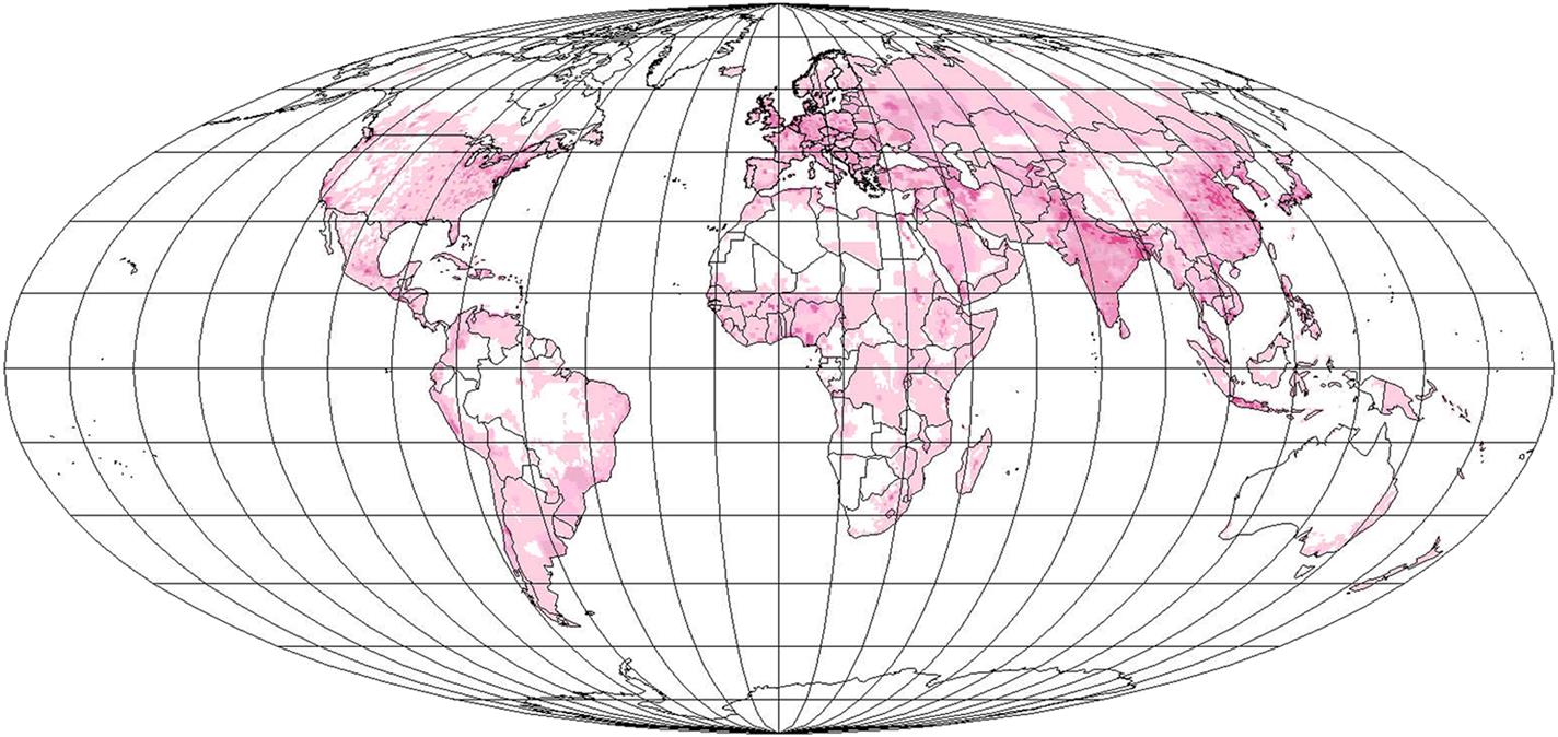
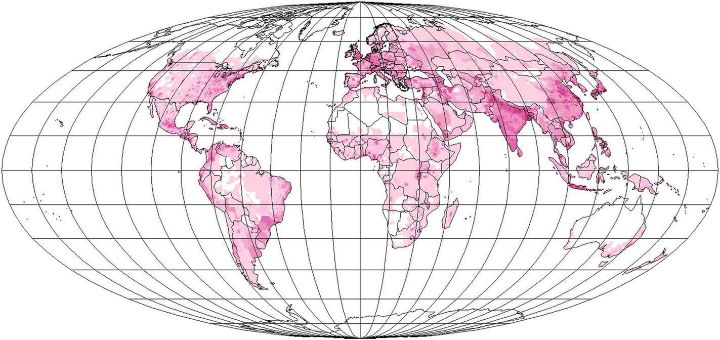
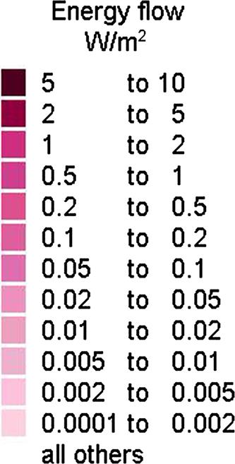
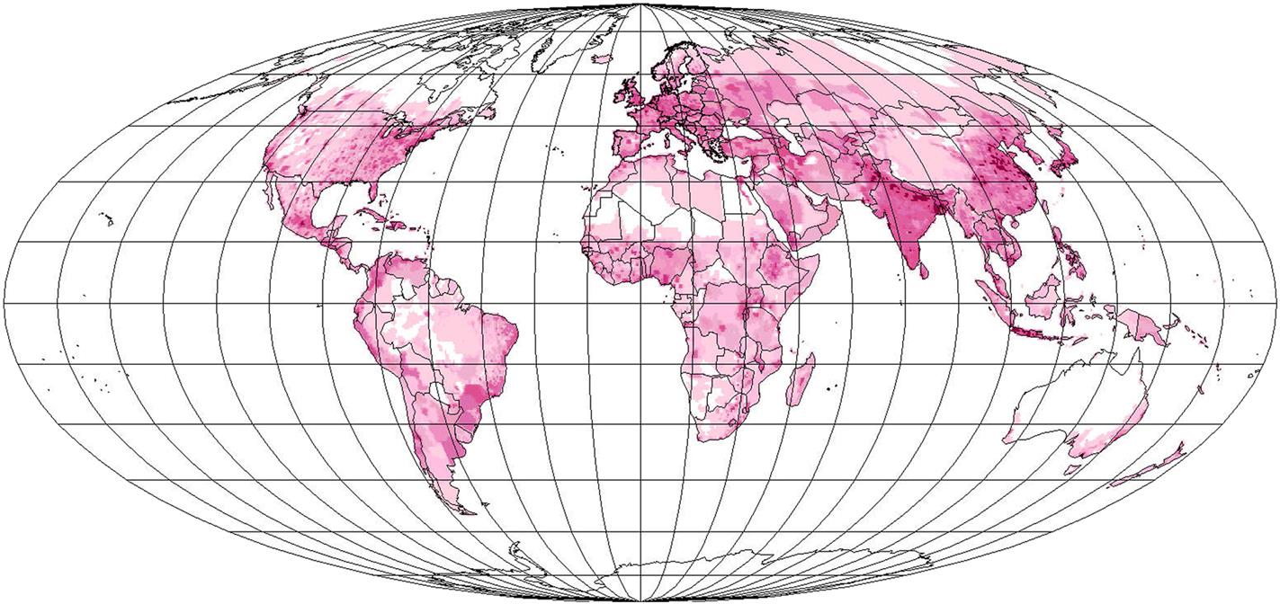
Figures 6.1 and 6.2 show the present and the assumed year-2050 population density, including the effect of increasing urbanization, particularly in developing regions, leading to 74% of the world’s population living in urban conglomerates by the year 2050 (United Nations, 1997). Discussion of energy use categories A to F above is expanded in the following survey.

6.2.3.1 Biologically acceptable surroundings
Suitable breathing air and shelter against wind and hot or cold temperatures may require energy services both indirectly, in the manufacture of clothes and habitable structures, and directly, in the provision of an active heat supply or a cooling system. Insulation by clothing makes it possible for humans to stay in cold surroundings with a modest increase in food supply (which serves to heat the layer between the body and the clothing). The main heating and cooling demands occur in extended spaces (buildings and sheltered walkways, etc.) intended for human occupation without the inconvenience of clothing or temperatures that would impede activities, such as manual labor.
Rather arbitrarily, but within realistic limits, it is assumed that fulfillment of goals related to shelter requires an average space of 40 m2 times a height of 2.3 m to be at the disposal of each individual in society and that this space should be maintained at a temperature of 18°C–22°C, independent of outside temperatures and other relevant conditions. As a “practical” standard of housing technology, for the heat loss P from this space I shall use the approximate form P=C×ΔT, where ΔT is the temperature difference between the desired indoor temperature and the outside temperature.
The constant C denotes a contribution from heat losses through the external surfaces of the space, plus a contribution from exchanging indoor air with outside air at a minimum rate of about once every 2 h. Half of the surfaces of the “person space” are considered external, with the other half being assumed to face another heated or cooled space. Best-current-technology solutions suggest that heat-loss and ventilation values of C=0.35 (heat loss)+0.25 (air exchange)=0.6 W °C−1 per m2 of floor area can be attained. The precise value, of course, depends on building design, particularly window area. The air exchange assumed above is about 40% lower than it would be without use of heat exchangers in a fraction of the buildings. The 40-m2 cap−1 assumed dwelling space is augmented below with 20 m2 cap−1 for other activities (work, leisure). Light is treated under activities.
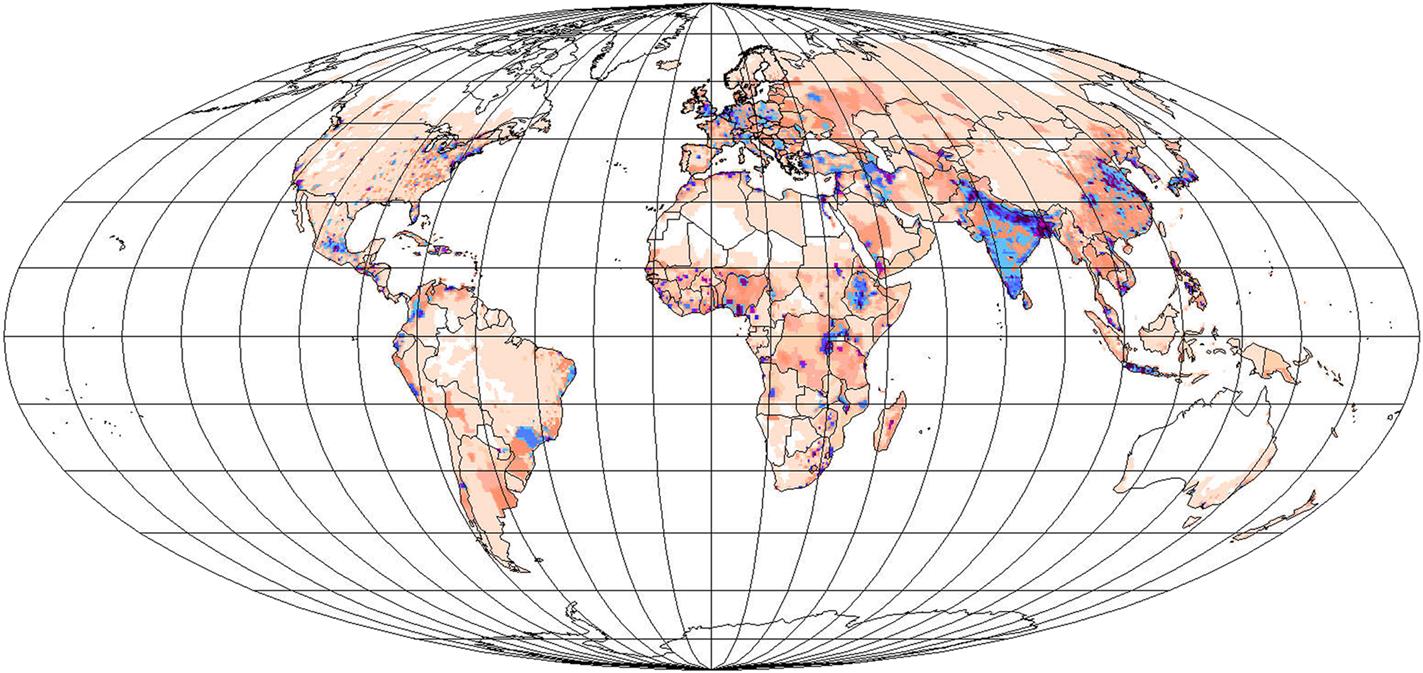
Now, energy needs* for heating and cooling, at a given location and averaged over the year, can be calculated with the use of climate tables giving the ambient temperature, e.g., hour by hour, for a typical year. If there are periods where temperatures are such that constant heating or cooling is required, the corresponding energy needs can be determined from the average temperatures alone. Heat capacity of the building will smooth out short-term variations, so that it is often a good approximation to determine heating and cooling demands from daily or even monthly average temperatures. An example of such estimations is shown in Figs. 6.3 and 6.4, for the annual heating and cooling requirements, separately, as a function of geographic location. The assumption is that space cooling is required for outdoor temperatures above 24°C and heating is required for temperatures below 16°C. Heat from indoor activities, combined with the thermal properties of suitable building techniques and materials, can provide indoor temperatures within the desired range of 18°C−22°C. Local space heating and cooling requirements are then obtained by folding the climate-related needs with the population density (taken from Fig. 6.2 for the year 2050 and used in the scenarios for the future described in section 6.7).


Here are a few examples: For Irkutsk, Siberia, the annual average temperature of −3°C gives an average dwelling energy requirement for heating of 651 W (per capita and neglecting the possibility of heat gain by heat exchangers included in Figs. 6.3 and 6.4). For Darwin, Australia, no heating is needed. These two values are taken as approximate extremes for human habitats in the summary table. Very few people worldwide live in harsher climates, such as that of Verkhoyansk (also in Siberia: average temperature, −17°C; heating requirement, 1085 W cap−1). Other examples are P=225 W cap−1 (New York City), P=298 W cap−1 (Copenhagen), and P very nearly zero for Hong Kong. Cooling needs are zero for Irkutsk and Copenhagen, while for Darwin, with an annual average temperature of 29°C, the cooling energy requirement is −P=209 W cap−1, assuming that temperatures above 22°C are not acceptable. The range of cooling energy demands is assumed to be roughly given by these extremes, from −P=0 to −P=200 W cap−1 For New York City, the annual average cooling requirement is 10 W cap−1 (typically concentrated within a few months), and for Hong Kong, it is 78 W cap−1.
6.2.3.2 Food and water
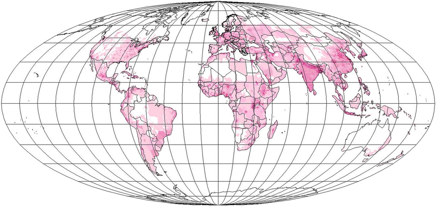
The energy from food intake corresponding to full satisfaction of food needs is about 120 W cap−1. Today, 28% of food intake is in the form of meat and other animal products (Alexandratos, 1995), but in the 2050 scenario presented below it is assumed that this fraction declines to 23%, partly owing to better balance in the diet of the industrialized regions and partly owing to an increased meat fraction in those regions presently having the lowest (e.g., East Asia, 9%). The distribution of food energy is shown in Figs. 6.5–6.6.


To store food adequately, the use of short- and long-term refrigeration is assumed. The average per capita food intake is of the order of 2×10⁻⁵ kg s−1, of which 0.8×10⁻⁵ kg s−1 is assumed to have spent 5 days in a refrigerator at a temperature ΔT=15°C below the surrounding room temperature, and 0.4×10⁻⁵ kg s−1 is assumed to have spent 2 months in a freezer at ΔT=40°C below room temperature. The heat-loss rate through the insulated walls of the refrigerator or freezer is taken as 2×10⁻² W°C−1 per kg of stored food. The energy requirement then becomes
plus the energy needed to bring the food down to the storage temperatures,
(assuming a heat capacity of 6000 J kg−1°C−1 above 0°C and half that value below the freezing point, and a phase change energy of 350 kJ kg−1). Energy is assumed to be delivered at the storage temperatures. Some energy could be regained from the melting of frozen food.
Cooking food requires further energy. Assuming that 40% of food intake is boiled at ΔT=70°C above room temperature, and that 20% of food intake is fried at ΔT=200°C above room temperature, the energy needed to bring the food up to the cooking temperatures is P~3.36+4.80=8.16 W cap−1, and the energy required for keeping the food cooking is P~1.45+2.08=3.53 W cap−1, assuming daily cooking times of 30 minutes for boiling and 15 minutes for frying (some food cultures certainly use more), and heat losses from the pot/pan/oven averaging 1 W°C−1 for the quantities of food cooked per person per day.
Provision of water involves pumping and cleaning/purification. The pumping and treatment energy needs are negligible on a per capita basis, but both are included in the industry sector considered below.
6.2.3.3 Security
Heating and cooling of buildings used by courts, police, military, and other security-related institutions are included as part of the 40 m2 area accorded each person. Remaining energy use for personal and national security would be for transportation and energy depreciation of materials and would hardly amount to more than 1 W cap−1, except for very belligerent or crime-ridden nations or nations with badly disliked regimes.
6.2.3.4 Health
Hot water for personal hygiene is taken as 50 liters day−1 cap−1 at T=40°C above the waterworks’ supply temperature, implying a rate of energy use averaging roughly P=97 W cap−1. Some of this heat could be recycled. Clothes washing and drying may amount to treating about 1 kg of clothes per day per capita. Washing is assumed to handle 5 kg of water/kg of clothes, at T=60° C (in practice, often more water is used, at different temperatures, some of which are closer to inlet temperature), or an average energy of P=15 W cap−1. For drying, it is assumed that 1 kg of water has to be evaporated (heat of evaporation about 2.3×10⁶ J kg−1) per day per capita, at an effective temperature elevation of 80°C (the actual temperature is usually lower, but mechanical energy is then used to enhance evaporation by blowing air through rotating clothes containers). Local air humidity plays a considerable role in determining the precise figure. Condensing dryers recover part of the evaporation heat, say, 50%. Energy use for the case considered is then 17 W cap−1. Hospitals and other buildings in the health sector use energy for space conditioning and equipment. These uses are included in household energy use (where they contribute 1%–2%).
6.2.3.5 Relations
Full goal satisfaction in the area of human relations involves a number of activities that are dependent on cultural traditions, habitats, and individual preferences. One possible example of a combination of energy services for this sector is used to quantify energy demands.
The need for lighting depends on climate and habitual temporal placement of light-requiring activities. Taking 40 W of present “state-of-the-art” commercial light sources (about 50 lumen per watt) per capita for 6 h/day, an average energy demand of 10 W cap−1 results. Still, radiant energy from light sources represents about 10 times less energy, and more efficient light sources are likely to become available in the future.
Radio, television, telecommunication, music, games, video, and computing, etc., are included in the scenario in section 6.7 and are assumed to take 65–130 W cap−1 (say 2–3 hours a day on average for each appliance), or an energy flux of 8–16 W cap−1. Add-on devices (scanners, printers, DVD burners, plus some not invented yet) increase demand, but increased efficiency of the new technology is assumed to balance the increased number of devices. Examples are flat-screen displays, which use 10–50 times less energy than the CRT screens that dominated at least television equipment up to the 1990s. Stand-by power for much of the equipment, as well as the power for computer screens and peripherals, was often not energy optimized by the end of the 1990s (cf. Sørensen, 1991). It is assumed that this will change in the future. Still, because the hoped-for balance between the increase in new equipment and their energy use is not proven, an additional energy expenditure of 30 W cap−1 was included in the section 6.7 scenario. The newer scenarios presented in section 6.5 have a much higher energy demand in this area (200 W cap−1), considering that, although efficiency increases, so do the sizes of television and computer screens, etc. In addition, permanent Internet access and automatization of a number of maintenance jobs in buildings could be among the reasons for increased energy use, although it would be coupled to reductions elsewhere in society. Social and cultural activities taking place in public buildings are assumed to be included above (electricity use) or under space conditioning (heating and cooling).
Recreation and social visits can entail a need for transportation, by surface or by sea or air. A range of 25–133 W cap−1 is taken to be indicative of full goal satisfaction: the higher figure corresponds to traveling 11 000 km y−1 in a road-based vehicle occupied by two persons and using for this purpose 100 liters of gasoline equivalent per year per person. This amount of travel could be composed of 100 km weekly spent on short trips, plus two 500 km trips and one 5000 km trip a year. Depending on habitat and where friends and relatives live, the shorter trips could be reduced or made on bicycle or foot, and there would be variations between cultures and individuals. Road congestion and crowded air space increase the likelihood of flattening out the current increase in transportation activity (as would teleconferencing and videophones), and transport is increasingly seen as a nuisance, in contrast to the excitement associated with early motoring and air travel. Road and air guidance systems would reduce the energy spent in stop-and-go traffic and in aircraft circling airports on hold. Hence, the lower limit of energy use for recreation and social visits is between 5 and 6 times less than the upper limit.
6.2.3.6 Activities
Education (understood as current activities plus lifelong continuing education required in a changing world) is assumed to entail building energy needs corresponding to 10% of the residential value, i.e., an energy flux of 0–20 W cap−1 for cooling and 0–65 W cap−1 for heating.
Construction is evaluated on the basis of 1% of structures being replaced per year, but the rate would be higher in periods of population increase. Measuring structures in units of the one-person space as defined above under Biologically acceptable surroundings, it is assumed that there are 1.5 such structures per person (including residential, cultural, service, and work spaces). This leads to an estimated rate of energy spending for construction amounting to 30–60 W cap−1 of stationary mechanical energy plus 7–15 W cap−1 for transportation of materials to building sites. The energy hidden in materials is deferred to the industrial manufacture and raw materials industry.
Agriculture, which includes fishing, the lumber industry, and food processing, in some climates requires energy for food crop drying (0–6 W cap−1), for water pumping in irrigation and other mechanical work (about 3 W cap−1), for electric appliances (about 1 W cap−1), and for transport (tractors and mobile farm machinery, about 6 W cap−1).
The distribution and service (e.g., repair or retail) sector is assumed, depending on location, to use 0–80 W cap−1 of energy for refrigeration, 0–150 W cap−1 for heating of commerce- or business-related buildings, about 20 W cap−1 of electric energy for telecommunications and other electric appliances, and about 5 W cap−1 of stationary mechanical energy for repair and maintenance service. Transportation energy needs in the distribution and service sectors, as well as energy for commuting between home and workplaces outside home, depend strongly on the physical location of activities and on the amount of planning that has been done to optimize such travel, which is not in itself of any benefit. Estimated energy spending is 30–100 W cap−1, depending on these factors. All the energy estimates here are based on actual energy use in present societies, supplemented with reduction factors pertaining to the replacement of existing equipment by technically more efficient types, according to the “best-available-and-practical technology” criterion, accompanied by an evaluation of the required energy quality for each application.
In the same way, energy use in manufacturing can be deduced from present data, once the volume of production is known. Assuming the possession of material goods to correspond to the present level in the United States or Scandinavia, and a replacement rate of 5% per year, leads to a rate of energy use of about 300 W cap−1. Less materialistically minded societies would use less. Spelled out in terms of energy qualities, there would be 0–40 W cap−1 for cooling and 0–150 W cap−1 for heating and maintaining comfort in factory buildings, 7–15 W cap−1 for internal transportation, and 20–40 W cap−1 for electric appliances. Most of the electric energy would be used in the production processes, for computers and for lighting, along with another 20–40 W cap−1 used for stationary mechanical energy. The assumed lighting efficiency is 50 lumen/W. Finally, the process heat requirement would include 10–100 W cap−1 below 100°C, 20–70 W cap−1 from 100°C to 500°C and 12–30 W cap−1 above 500°C, all measured as average rates of energy supply over industries very different in regard to energy intensity. Some consideration is given to heat cascading and reuse at lower temperatures, in that the energy requirements at lower temperatures have been reduced by what corresponds to about 70% of the reject heat from the processes in the next higher temperature interval.
Most difficult to estimate are the future energy needs of the resource industry. This is for two reasons: one is that the resource industry includes the energy industry and thus will vary greatly depending on what the supply option or supply mix is. The second reason is the future need for primary materials: will it be based on new resource extraction, as is largely the case today, or will recycling increase to near 100% (for environmental and economic reasons connected with depletion of mineral resources)?
As a concrete example, let us assume that renewable energy sources are used, as in the scenario considered in section 6.4. Extraction of energy by the mining and oil and gas industries as we know them today will disappear, and activities related to procuring energy will take a quite different form, related to renewable energy conversion equipment, which in most cases is more comparable to present utility services (power plants, etc.) than to a resource industry. This means that energy equipment manufacturing will become the dominant energy-requiring activity.
For other materials, the ratios of process heat, stationary mechanical energy, and electricity use depend on whether mining or recycling is the dominant mode of furnishing new raw materials. In the ranges given, not all maxima are supposed to be realized simultaneously, and neither are all minima. The numbers are assumed to comprise both the energy and the material provision industries. The basis assumption is high recycling, but for the upper limits not quite 100%. There will therefore be a certain requirement for adding new materials for a growing world population. The assumed ranges are 0–30 W cap−1 for process heat below 100°C as well as for 100°C–500°C, 0–250 W cap−1 above 500°C, 0–170 W cap−1 of stationary mechanical energy, 0–30 W cap−1 of electric energy and 0–20 W cap−1 of transportation energy.
6.2.3.7 Summary of end-use energy requirements
Table 6.5 summarizes, by main energy qualities, the estimates of energy delivered to end-users in the scenario discussed for year 2050. The 2050 per capita energy services are more than twice those of today, and yet the average energy delivered to each end-user is only half that of today, owing to higher efficiency of each conversion step. In section 6.7, the primary energy required for the global 2050 scenario is determined, while the regional studies in section 6.6 use updated end-use estimates.
Table 6.5
Energy delivered to end-user in 2050 scenario, including environmental heat (Sørensen and Meibom, 1998).
| Regions: / Energy Quality: | 1. USA, Canada | 2. Western Europe, Japan, Australia | 3. Eastern Europe, Ex-soviet, Middle East | 4. Latin America, SE Asian “tigers” | 5. China, Rest of Asia | 6. Africa | Average & Total |
| Food based on animals | 30 | 30 | 30 | 25 | 25 | 20 | 23% |
| 45 | 45 | 45 | 37 | 37 | 25 | 36 W/cap | |
| 17 | 24 | 47 | 52 | 148 | 51 | 339 GW | |
| Food based on grain & vegetables | 70 | 70 | 70 | 75 | 75 | 80 | 77% |
| 119 | 119 | 119 | 128 | 128 | 114 | 123 W/cap | |
| 45 | 63 | 124 | 177 | 506 | 232 | 1148 GW | |
| Gross transportation energy | 359 | 299 | 140 | 201 | 99 | 30 | 125 W/cap |
| 136 | 158 | 146 | 277 | 392 | 61 | 1170 GW | |
| Heat pump input for low-temp. heat and cooling | 110 | 110 | 87 | 43 | 80 | 22 | 65 W/cap |
| 58 | 58 | 90 | 60 | 318 | 45 | 610 GW | |
| Environmental heat | 240 | 256 | 203 | 100 | 186 | 51 | 151 W/cap |
| 91 | 135 | 210 | 140 | 741 | 105 | 1421 GW | |
| Direct electric & all other energy | 420 | 424 | 245 | 288 | 283 | 47 | 240 W/cap |
| 153 | 224 | 255 | 398 | 1116 | 96 | 2242 GW | |
| Total delivered energy | 1272 | 1252 | 838 | 800 | 814 | 290 | 742 W/cap |
| 482 | 661 | 871 | 1104 | 3225 | 591 | 6934 GW | |
| Population 2050 | 379 | 528 | 1040 | 1380 | 3960 | 2040 | 9340 millions |
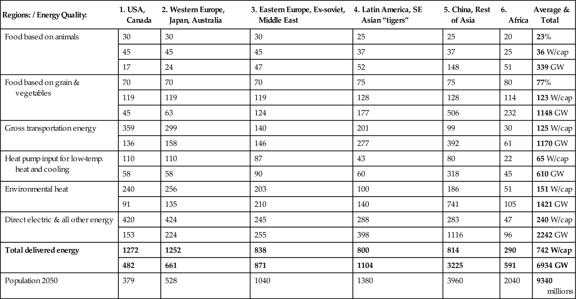
The energy delivered differs from end-use energy by losses taking place at the end-users’ location.
Table 6.5 gives the gross energy input to transportation needs, accumulating the individual demands for personal transportation, for work-related transport of persons and goods, and for transport between home and work (“commuting”). The net energy required to overcome frictional resistance and the parts of potential energy (for uphill climbing) and acceleration that are not reclaimed is multiplied by a factor of 2 to arrive at the gross energy delivery. This factor reflects an assumed 2050 energy conversion efficiency for fuel-cell-driven (with electric motor) road vehicles of 50%, as contrasted with about 20% for present-day combustion engines. For the fraction of vehicles (presumably an urban fleet) using batteries and electric drives, the 50% efficiency is meant to reflect storage-cycle losses (creep current discharge during parking and battery-cycle efficiency). The geographical distribution of transportation energy demands is shown in Fig. 6.9.
The row “direct electric and all other energy” in Table 6.5 comprises medium- and high-temperature heat, refrigeration other than space cooling (which is included in the space-heating and space-cooling energy), stationary mechanical energy, and dedicated electric energy for appliances and motors outside the transportation sector. For these forms of energy, no end-use efficiency is estimated, as the final service efficiency depends on factors specific to each application (re-use and cascading in the case of industrial process heat, sound- and light-creating technologies, computing, and display and printing technologies, all of which are characterized by particular sets of efficiency considerations). The geographical distribution of these energy requirements in the 2050 scenario is shown in Fig. 6.8. The distribution of the electric energy input to heat pumps (COP=3), which in the scenario covers space heating, cooling, and other low-temperature heat demands, is shown in Fig. 6.7, and Fig. 6.10 adds all the scenario energy demands, including environmental heat drawn by the heat-pump systems. The low COP assumed for heat pumps reflects the location of the corresponding loads at high latitude, where suitable low-temperature reservoirs are difficult to establish.


Estimations of future energy demands are obviously inaccurate, due to both technical and normative factors: on the one hand, new activities involving energy use may emerge, and, on the other hand, the efficiency of energy use may be further increased by introduction of novel technology. Yet it is reassuring that the gross estimate of energy demands associated with full goal satisfaction (for a choice of goals not in any way restrictive) is much lower than present energy use in industrialized countries. It demonstrates that bringing the entire world population, including little-developed and growing regions, up to a level of full goal satisfaction is not precluded for any technical reasons. The scenarios in section 6.4 are consistent with this, in assuming energy-efficiency gains of about a factor of 4.
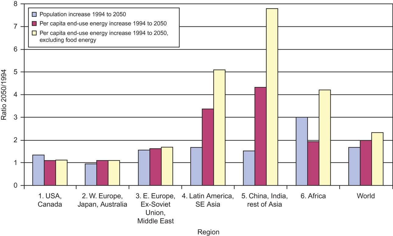
Figure 6.11 illustrates the reference scenario assumptions in different regions by comparing end-use energy, with and without food energy, between 2050 and 1994 populations. Compared to many other scenarios (see, for example, WEA, 2000), the 2050 scenario used here places more emphasis on using the most efficient technology. The reason for this is an assumption of economic rationality that strangely contrasts with observed behavior: Current consumers often choose technology that entails a much higher cost for energy inputs during the operation life than the increased cost they would need to pay at purchase for the most energy-efficient brand of the technology in question. This economic irrationality pervades our societies in several other ways, including the emphasis in RD&D programs on supply solutions that are much more expensive than solutions directed at diminishing energy use. Thus, the “growth paradigm” seems to be so deeply rooted in current economic thinking that many people deem it “wrong” to satisfy their needs with less energy and “wrong” to invest in technology that may turn their energy consumption on a declining path. This problem is rarely discussed explicitly in economic theory, but is buried in terms like “free consumer choice,” and is coupled with encouraging the “freedom” of advertisement, allowing substandard equipment to be marketed without mention of the diseconomies of its lifetime energy consumption.
One wonders when consumers will, instead, respond with the thought that, “If a product needs to be advertised, there must be something wrong with it”? Either the product does not fulfill any need, or it is of lower quality than other products filling the same need with lower energy consumption. New, fairly expensive energy-production technology, such as solar or fuel cells, get much more media attention than freezers with a four-times-lower-than-average energy consumption. Given that world development at present is not governed by economic rationality, the supply–demand matching exercises presented in the following subsections, which are based on the scenarios defined according to the principles set forth above, will take up the discussion of robustness against underestimates of future energy demand.
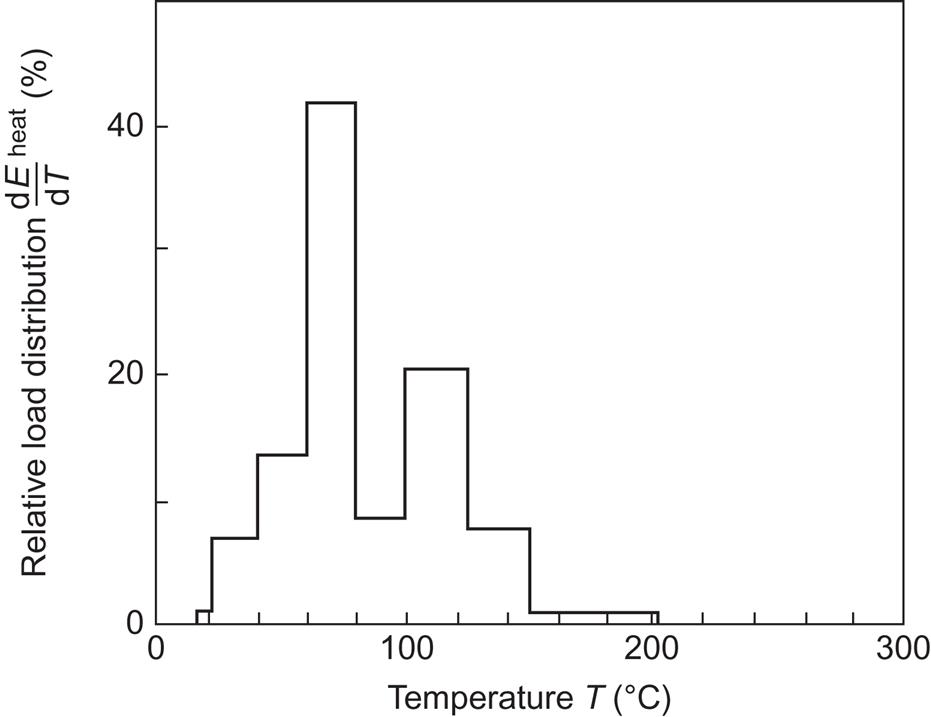
Specification of the energy form required at the end-user first amounts to distributing the sector loads on electric, mechanical, heat, radiant energy, etc., but the heat energy demand must be further specified, as described above, in order to provide the type of information needed for planning and selecting the energy systems capable of serving the loads. As an example of the investigations needed, Fig. 6.12 shows the temperature distribution of heat demand for the Australian food-processing industry.
6.2.3.8 Patterns of time variations
In a complex system with decisions being taken by a large number of individual consumers, the time pattern of the load cannot be predicted precisely. Yet the average composition and distribution of the load are expected to change smoothly, with only modest ripples appearing relative to the average. However, there may be extreme situations, but with a low probability of occurrence, that should be taken into account in designing energy system solutions.
Fluctuations in electricity demand have routinely been surveyed by utility companies, many using simulation models to optimize use of their supply system. Figure 6.13 gives two examples of seasonal variations in electricity loads, one being for a high-latitude area, exhibiting a correlation with the number of dark hours in the day, and the other being for a metropolitan area in the southern United States, reflecting the use of electricity for space-cooling appliances.

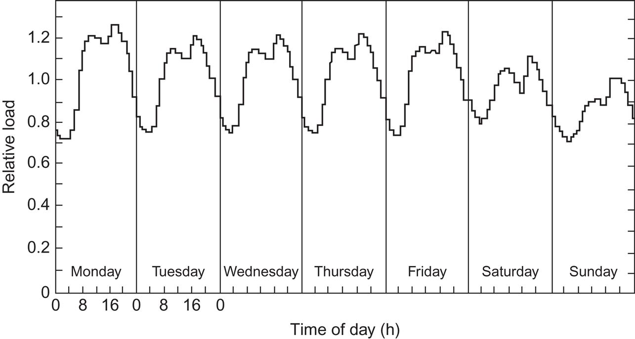
Superimposed on seasonal variations is a daily cycle, which often exhibits different patterns on weekdays versus weekends. The example given in Fig. 6.14 (also from the United States) shows a further irregularity for Mondays (a “peak working day”), probably reflecting a higher energy requirement for the “cold starts” of industrial processes relative to continual operation during the following days. Yet, not all regions exhibit a pronounced “peak working day” load like the one in Fig. 6.14. Figure 6.15 shows the daily load variations at Danish utilities for a summer and a winter weekday. The ratio between the maximum and the minimum load is considerably higher than in the American example in Fig. 6.14, presumably because a higher proportion of industries in the United States require continuous operation. A detailed investigation of time variations in demand and its implication for energy supply system design is made in Sørensen (2015).

In connection with renewable energy sources, a particularly attractive load is one that need not be performed at a definite time but can be performed anywhere within a certain time span. Examples of such loads (well known from historical energy use) are flour milling, irrigation, and various household tasks, such as bathing and washing. The energy-demand patterns for many such tasks rest on habits that, in many cases, developed under the influence of definite types of energy supply and that may change as a result of a planned or unplanned transition to different energy sources. Distinction between casual habits and actual goals requiring energy conversion is not always easy, and the differentiation is a worthy subject for social debate.
Data on renewable energy flows (or reservoirs) that may serve as inputs to the energy conversion system are a major theme of Chapter 2 and particularly of Chapter 3.
As mentioned in section 6.1, the performance of most conversion systems can be calculated with sufficient accuracy by a “quasi-steady-state approximation,” and most of these systems possess “buffering mechanisms” that make them insensitive to input fluctuations of short duration (such as high-frequency components in a spectral decomposition). For this reason, input data describing renewable energy fluxes may be chosen as time averages over suitable time intervals. What constitutes a “suitable” time interval depends on the response time (time constant) of the conversion system, and it is likely that the description of some systems will require input data of a very detailed nature (e.g., minute averages), whereas other systems may be adequately described using data averaged over months.
A situation often encountered is that the data available are not sufficient for a complete system simulation on the proper time scale (i.e., with properly sized time steps). Furthermore, interesting simulations usually concern the performance of the system some time in the future, whereas available data by necessity pertain to the past. Demand data require that a model be established, while, for resource data, it may be possible to use “typical” data. “Typical” means not just average data, but data containing typical variations in the time scales that are important for the contemplated energy conversion system.
Examples of such data are hourly values of wind velocities selected from past data, which, incorporated into a simulation model, may serve to estimate system performance for future years. Clearly, this type of “reference year” should not contain features too different from long-term statistics.
For some renewable energy systems, e.g., hydroelectricity, the variations between years are often important system design parameters.
Synthetic databases (e.g., covering a year) have been constructed by combining sequences of actual data picked from several years so that averages of important variables take values close to their long-range averages, but such that “typical” fluctuations are preserved in the data. Reference year solar radiation and other meteorological data, which are made available for engineering purposes for selected locations (notably certain cities in Europe and North America, cf. section 3.1.3), are an example.
For computer simulations, standard procedures exist that will generate random numbers with a specified distribution (e.g., Gaussian) once the fluctuation (or “half-width”) and average value of the distribution are specified. This approach may be described as a stochastically generated database. It has found widespread application, e.g., in prediction of wind turbine production characteristics (Sørensen, 1986; Troen and Petersen, 1989).
6.3 Supply scenario construction
In the construction of scenarios, it is necessary to have data for the energy supply sources intended for inclusion, and it is often convenient to create a source database of potential production profiles to pick from when piecing together a scenario. An overview of common elements of such a resource-exploitation database is given below.
6.3.1 Photovoltaic power production
A solar radiation model is constructed on the basis of data for solar radiation incident on a horizontal plane. One set of data, from NASA, is based on analysis (Pinker and Laszlo, 1992) of satellite measurements of radiation, albedo (reflectance), cloud cover, and attenuation of radiation in the air (NASA, 1997). The other study considered here collects many types of weather and climate data (NCEP–NCAR, 1998) and uses balance equations and a global circulation model (horizontal resolution about 210 km and 28 vertical levels) to improve the data’s consistency (Kalnay et al., 1996). However, for solar radiation, this study does not use ground-based observations, so, again, the solar radiation data are based on top-of-the-atmosphere fluxes and various absorption, reflection, and attenuation processes plus the balance requirements at the Earth’s surface. The two types of analysis give similar results for solar radiation. The balance equations (which take the difference between upward and downward short- and long-wavelength radiation and heat fluxes) do suggest too high an albedo over oceans, but the land data that are used here appear to be reliable. Figure 3.1 shows the radiation on a horizontal plane at the Earth’s surface for selected months of 1997 (NCEP–NCAR, 1998). In order to calculate the solar radiation incident on inclined surfaces, such as the ones characterizing most solar installations, ideally one would have hourly data for direct and scattered radiation (or equivalently for direct and total global radiation). Then, to estimate the value of scattered radiation for differently inclined surfaces, one would assume that the scattered radiation is uniform. For direct radiation, ray calculations with the appropriate angles between the direction to the sun and the normal to the collector surface have to be performed hourly. Such calculations have been performed and compared with measurements on inclined surfaces at several major solar installations and some weather stations (see Chapter 3). Such data are not globally available but can be approximately inferred from available radiation data, as is done in Figs. 3.14–3.15. These data will be used in the scenarios discussed in section 6.6.
The task is to estimate the radiation on a surface tilted either north or south by an angle approximately equal to the latitude (as this gives the optimum performance) on the basis of the horizontal surface solar radiation data available. Only a modest accuracy is required because of the characteristics of the actual solar installations used in the scenarios:
1. Building-integrated solar panels will be influenced by the structure of the building: some solar panels will be mounted on vertical facades, while others will be placed on roofs that are either flat or tilted, typically 30°, 45°, or 60°. In all cases, the panels’ actual orientation may not be precisely south or north, although the resource estimates are here given only for buildings facing approximately correctly and not being exposed to strong shadowing effects from other structures. The penalty for incorrect orientation and tilt angle is usually modest and mostly influences seasonal distribution of power (cf. Chapter 3).
2. Centralized solar farms are generally oriented optimally, using total production maximization for panels not tracking the sun. However, the majority of locations suited for central photovoltaic (PV) installations are the desert areas of the Sahara, the Arabian Peninsula, the Gobi, and Australian inland locations. Because they are all fairly close to the Equator, there is modest seasonal variation in solar radiation, and horizontal-surface data are often quite representative.
The early scenarios presented in section 6.7 used the following simple approximation, originating from the analysis of the Danish (latitude 56°N) data given in Fig. 3.17. Here the radiation on a latitude-inclined surface in January and July very nearly equals the horizontal radiation in October and April, whereas the horizontal-surface data for January and July are lower and higher than the inclined-surface measurements, respectively. The October and April horizontal data are thus used as a proxy for January and July inclined-surface radiation, and the April and October inclined-surface values are constructed as simple averages of the January and July adopted values. This procedure, which works well for the Danish latitude, is also less inaccurate for low latitudes, because of the relative independence of seasons mentioned above, and we simply use it for all locations.
Figure 2.24 shows the NCEP–NCAR (1998) data for a horizontal surface. An alternative calculation using the European general circulation model HADCM2-SUL (Mitchell and Johns, 1997) gave very similar monthly 1997 solar radiation values.
In order to derive the actual energy extracted from PV solar panels, a fixed conversion efficiency of 15% is assumed. This is a fairly conservative estimate for the year-2050 technology, considering that the current efficiency of the best monocrystalline cells is above 20% and that of amorphous cells is near 10%, with multicrystalline cells falling in between. The 2050 choice is likely to be thin-film technology, but not necessarily amorphous or group III–V based, as new techniques allow crystalline or multicrystalline silicon material to be deposited on substrates without the complicated process of ingot growth and cutting. The efficiency of such cells is lower than that of the best current crystalline cells, but increasing, and since 2002, multicrystalline cells have surpassed monocrystalline cells in worldwide shipments.
Finally, the availability of sites for mounting PV panels either in a decentralized fashion or centrally in major energy parks is estimated: the decentralized potential is based on availability of suitably inclined, shadow-free surfaces. The area of suitably oriented surfaces that may be used for building-integrated PV energy collection is assumed to be 1% of the urban horizontal land area plus 0.01% of cropland area. The latter reflects the density of farmhouses in relation to agricultural plot sizes and is based on European estimates, roughly assuming that 25% of rural buildings may install solar panels. Potential PV production is thus taken as 15% of radiation times the fraction of the above two area types and the stated percentage for each. A final factor of 0.75 is applied in order to account for transmission and storage-cycle losses, assuming about 5% transmission losses and that roughly half the energy goes through a storage facility of 60% round-trip efficiency (e.g., reversible fuel cells). The flow of energy reduced by all these factors represents the energy delivered to the end-use customers in the form of electricity. It is shown in Fig. 6.16 for two months, with regional sums being discussed in section 6.7.

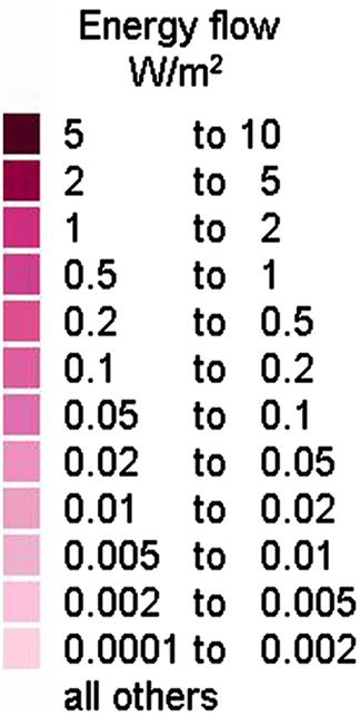

For the centralized PV possibility, the potential is taken as that derived from 1% of all rangeland plus 5% of all marginal land (deserts and scrubland), again times 15% of the incoming radiation and times 0.75 to account for transmission and storage losses. As shown in Fig. 6.17, this is a huge amount of energy, and it shows that such centralized PV installations can theoretically cover many times the demand of our 2050 scenario. Setting aside 1% of rangeland incurs only an insignificant reduction in other uses of the land, even for a small number of large plants. The same is true for desert and marginal land, where only the 5% most suitable area needs to be used, which in reality might be 10% when the entire installation is included (including frames, access roads), of which the solar panels are only part. A centralized installation in the huge area of the Sahara Desert would suffice to supply more than the entire world’s need for energy. Of course, it would require intercontinental transmission, which may be realistic by the year 2050, e.g., through superconducting trunk lines (Nielsen and Sørensen, 1996; Sørensen, 2015).

6.3.2 Wind-power production
There have been substantial advances in data availability for estimating wind-power production at any location on the Earth. The scenarios in section 6.6 use scatterometer and new re-analysis data discussed below, available on a 6-hour basis for 0.5° longitude or latitude grids. When the earlier scenarios of section 6.7 were simulated, only monthly averaged wind data were available, and the following coarse approximation was used to arrive at useful data:
The basic data used in the 1998 calculation of potential wind-power production are from a 1997 re-analysis of meteorological station data and altitudinal data from balloons and aircraft, analyzed according to the method of Kalnay et al. (1996) and using a general circulation model to improve consistency (NCEP–NCAR, 1998). For the scenario, simple average pressure levels of 1000 mb and 925 mb were used to represent the wind speeds at typical turbine hub heights of around 70 m. However, as the data are monthly mean wind speeds <v> constructed based on zonal and meridional winds, we need a model of the relationship between <v>3 and <v3> to go from wind speeds to power in the wind. Simple models imply a rough proportionality between these two quantities, as used, for example, in the U.S. wind atlas prepared by the Pacific NW Laboratory (Swisher, 1995) and also in the Weibull distribution approach of the European wind atlas (Troen and Petersen, 1989). Inspired by these sources, one may estimate the relation between the power in wind Pw and the wind speed v (m s−1) from the relation
The power in the wind obtained in this way is illustrated in Fig. 3.27 for the four seasons. The results in the figure may be compared with the outcome of using the new 6-hour data below, in which case no ad hoc approximation is needed to get from wind speeds to power in the wind, because the data are not averages over 6 hours, but instantaneous values measured every 6 hours (well, actually every 12 hours, see the reason below).
Going from the power in the wind to the power that may be produced by a wind turbine, the non-linear response of wind turbines has to be taken into consideration. Turbines of modern design aim at a high annual production and typically start producing only at around 5 m s−1; they reach a fixed maximum production at around 12 m s−1. Thus, there would not be any production for a monthly average wind speed below 5 m s−1, if it were made up of nearly constant values throughout the time range. However, actual time-series of wind speeds reflect the passage of weather fronts, typically oscillate with periods of about 2 weeks, and entail power production from the above type of wind turbine at practically all monthly average wind speeds, down to zero. The approach is then to parameterize the average power production from wind turbines as
representing contemporary wind turbine constructions through a power factor slightly above current levels. Owing to the coarseness of the GIS* grids used in 1998 (for wind-speed data for approximately 300 km cells at the Equator, diminishing by the cosine of the latitude toward the poles), the method does not at present compete with wind atlas methods available in certain parts of the world. The 2008 scatterometer plus re-analysis data are better, but still with a grid size of 25 km, which leads to an expected power production accuracy of around 100 km. This is, however, sufficient for planning purposes. The use of general circulation models in recalculating the data ensures that both surface roughness and general circulation determinants are included.
It should be noted that the data from low-height meteorological stations (which are often at sheltered locations at or under 10 m and are a substantial source of the data underlying the NCEP-NCAR data), relative to elevated data at typical wind turbine hub heights, may lead to a poor representation of actual wind conditions in a given area. For this reason, the European wind atlas used only selected station data believed to be more relevant for wind turbine exploitation. However, comparison with the Hadley model data, which have only a weak dependence on station data because they are generated from a general circulation model using topological features of wind roughness (friction), indicates that the method is quite reliable. The reason for this is presumably that we use pressure-level data for both of the two lowest model pressure levels, rather than the 10 m data also available in the NCEP-NCAR database. Repeating the calculation for the 10 m data indeed gives a considerably stronger dependence on the dubious ground-level measurements.
The final step in estimating potential production from wind turbines in the scenario is to appraise the locations suited for erection of wind turbines. They are divided into three categories: decentralized wind-power production on farmland, and centralized production in wind parks, either onshore or offshore. For decentralized production, we assume that a (vertical) turbine-swept area amounting to 0.1% of cropland and rangeland areas may be used for wind production. Only the part of cropland designated “open cropland” (cf. section 6.3.3) is used. This excludes mixed forest and cropland, where trees are likely to impede wind flow. The assumed density of turbines corresponds roughly to the current density of wind turbines in many parts of Denmark, although the current turbines’ average size is smaller than that of the turbines envisaged for the mid-21st century.
Currently, new turbines are typically of unit size above 2 MW and have a hub-height of at least 50–60 m. Owing to the combination of swept area increasing as the square of the linear dimension and wind speeds increasing with height, the 2–5 MW turbines envisaged in the 2050 scenario will not be conspicuously larger than those of the current generation.
In terms of ownership, the density of decentralized turbines in the scenario would correspond to 1 out of 5–10 farmers owning a wind turbine (with large variations due to farm size variations between regions). Current wind-power utilization in the country with highest per capita wind-power production, Denmark, still collects a substantial amount of power from farm-situated wind turbines. In many other countries, the emphasis has been on centralized production from turbine clusters. The amount of decentralized wind-power potentially available is shown in Figs. 6.18 and 6.19. Strong seasonality is evident, and repeating the evaluation using data for years other than 1997 indicates that variation between years is also large.


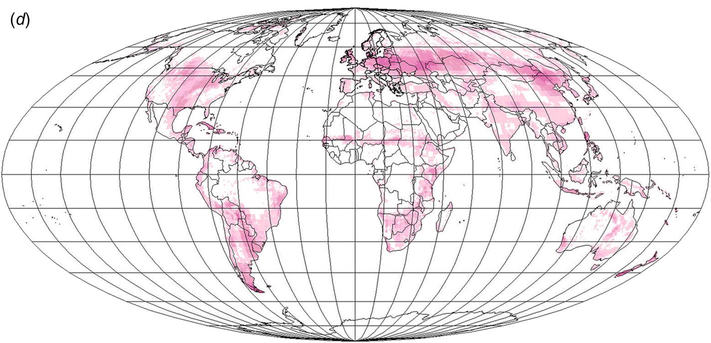
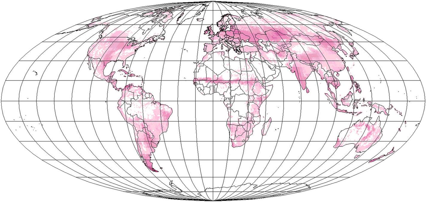
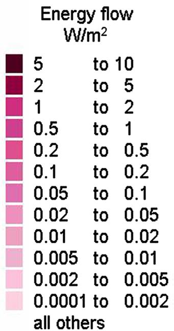
Centralized wind-power is here understood as power not produced in connection with individual farms. For land-based wind parks, only placement on marginal land is accepted in the global scenario. In contrast to photovoltaic power, there is a fundamental limit to the fraction of land that can be used for wind-power extraction, owing to shadowing and interference between wake flows that create turbulence and reduce the power output.
This limit would be a vertical swept area of about 1% of the horizontal land area (Sørensen, 1995). The scenario assumes that only 10% of the marginal land areas are used for placement of wind turbines at such spacing, implying a maximum swept area constituting 0.1% of the land area. This is small enough not to interfere with other uses of the marginal land, such as the solar cell parks considered in section 6.3.1. Figure 6.20 gives the annual production that potentially may be derived from such wind parks.

Finally, the scenario considers offshore wind parks, meaning turbines placed in shallow waters at a distance from the shore that minimizes visual impact. This mode of wind utilization has become popular in recent years, as innovative low-cost solutions to the offshore foundation problem have been found (Sørensen, 1995). In order to obtain an estimate for the potential, offshore water bodies with a depth less than 20 m are first identified (Fig. 6.21). Of these, it is assumed that only 10% can be used for wind-power generation, owing to competing uses (fishing, military, ship routes, etc.). Again taking into account the 1% maximum utilization rate imposed by turbine interference, one arrives at a 0.1% maximum use of offshore locations for wind-power extraction. The average amount of power that can be derived from these locations is shown in Fig. 6.22. There are an additional number of inland water bodies that could also be used for wind-power production, but they are disregarded here due to their possible recreational value.


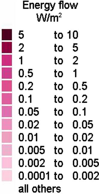
6.3.2.1 Industry development
The assumptions about future hub height, power characteristics, and capacity factors made in the scenarios are based on the choices made by current manufacturers and trends appearing in the history of the wind industry, with emphasis on recent behavior.
Wind turbines have been in substantial use for more than 1000 years, with early text evidence in China and India and the earliest pictures being from Persia around 1300. The earliest were all vertical axis machines, spreading to the Mediterranean region of Europe, while horizontal axis machines were developed in England, Holland, Denmark, the Baltic region, and Russia (cf. overview of wind history in Sørensen, 1995). In the 16th century, cities like Copenhagen had about 100 turbines with a hub height of greater than 10 m that were used for grinding flour just outside the city walls, and, in Holland, some wind turbines were used to pump water as part of the drainage system for lowlands. Around 1900, wind turbines played a significant role in powering new settlements in the North American plains and Australian outposts, and the first hydrogen- and electricity-producing wind turbines were tested in Denmark (La Cour 1900; cf. Hansen, 1985). The DC electricity-producing wind turbines kept competing with coal-based power during the first decades of the 20th century, but they were gradually used only on island sites and eventually they lost there, too, as undersea cables became extended to most Danish islands. By the end of the 1920s, Denmark had about 30 000 wind turbines, three times as many as today. Experiments with AC-generating wind turbines were made before and after World War II, with a comeback in several European countries following the 1957 closure of the Suez Canal (blocking transport of the Middle East oil then used in European power stations). The 200 kW Gedser turbine was technically successful (Juul, 1961), and it served as a model for the subsequent resurrection of wind turbine manufacture following the oil supply cuts in 1973/1974. Since 1974, development has experienced decreasing cost and rapidly increasing installed capacity, as stated in section 1.1.
Figure 6.23 shows the development in turbine size (height and swept diameter) of commercial wind turbines since 1980, and Fig. 6.24 shows corresponding trends in rated capacity and specific power production at the locations of typical Danish installations. Figure 6.23 also shows the capacity factor (average power produced over rated power) averaged over all turbines operated in Denmark at a given time, and the much higher capacity factor achieved by some new, offshore wind farms. From 2010 and onwards, manufacturers have offered turbines of 5–8 MW rated power. These large turbines make extraordinary demands on blade materials, causing the glass- or wood-fiber blades previously used to be replaced by advanced fiber technologies. Also, advanced computerized control and generator technologies have made it possible to use direct drives and variable-speed rotors, allowing the variable wind speeds to initially generate AC of varying frequency, which is subsequently transformed to a fixed frequency, typically by way of DC as intermediary power form.
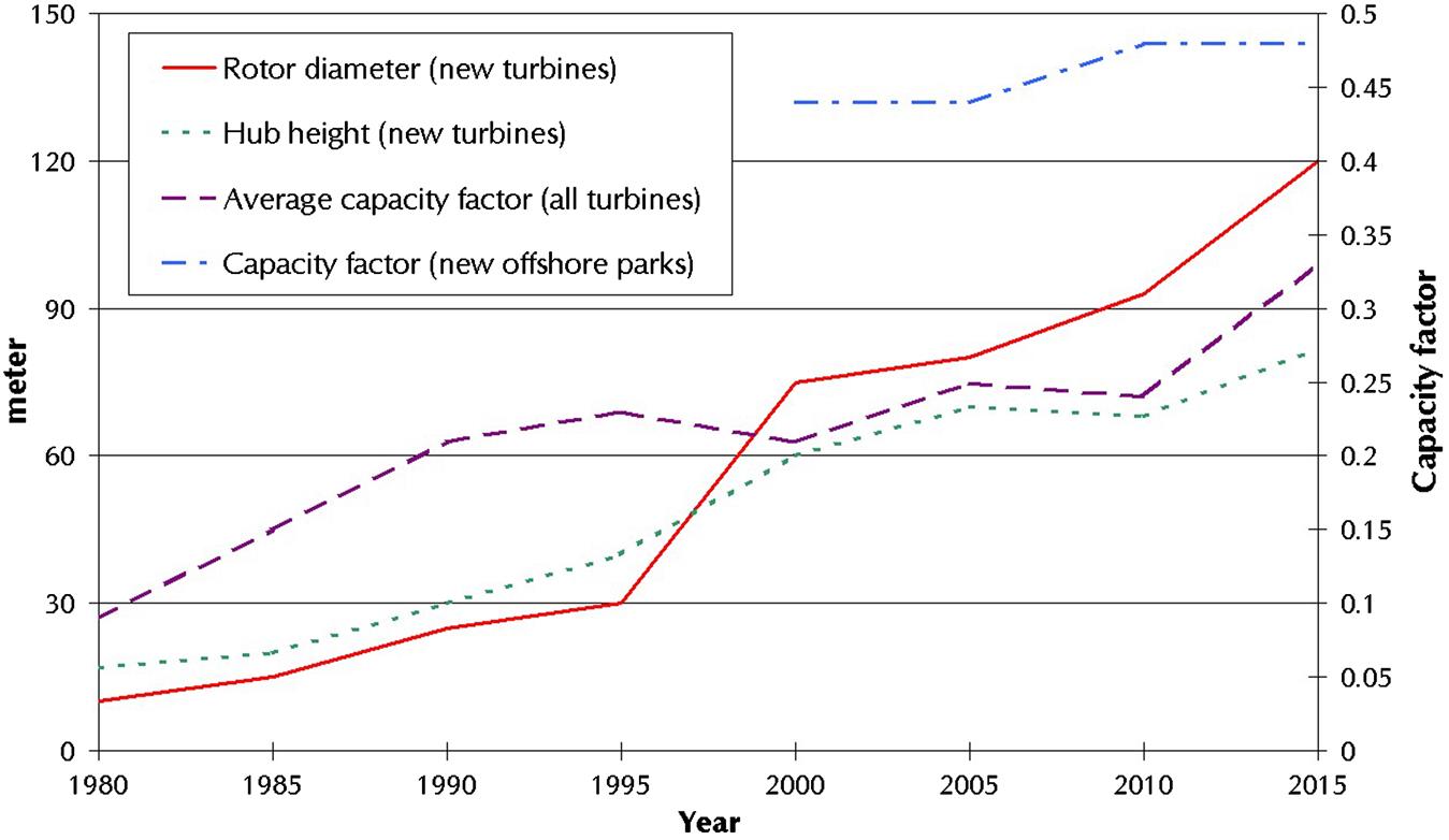
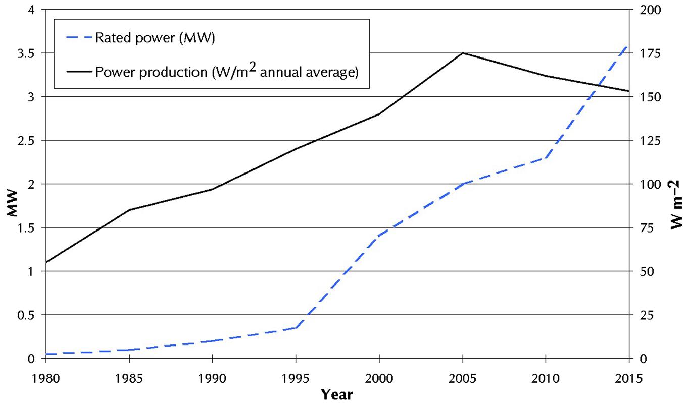
The power curve (output as function of wind speed) for the currently newest large wind turbines (7–8 MW) is shown in Fig. 6.25, along with the power curve used in the regional scenario simulations in section 6.6, made to maximize annual production at good wind sites. The fact that manufacturers in recent decades have departed from the philosophy of aiming for the largest annual production is based on the fact that many international customers are power utilities with weak power transmission capacities to neighboring regions and no energy storage facilities capable of storing and regenerating electricity. In this situation, it seems better to aim for as many operating hours during a year as possible (using a wing blade profile that allows the turbine to produce power also at low wind speeds), even if such blade profiles does not maximize the annual production. This remedy is very partial, as there will still be substantial variations in output over the year, and having a large fraction of power demands covered by wind still requires consideration of techniques to deal with intermittency of supply (Sørensen, 2015).
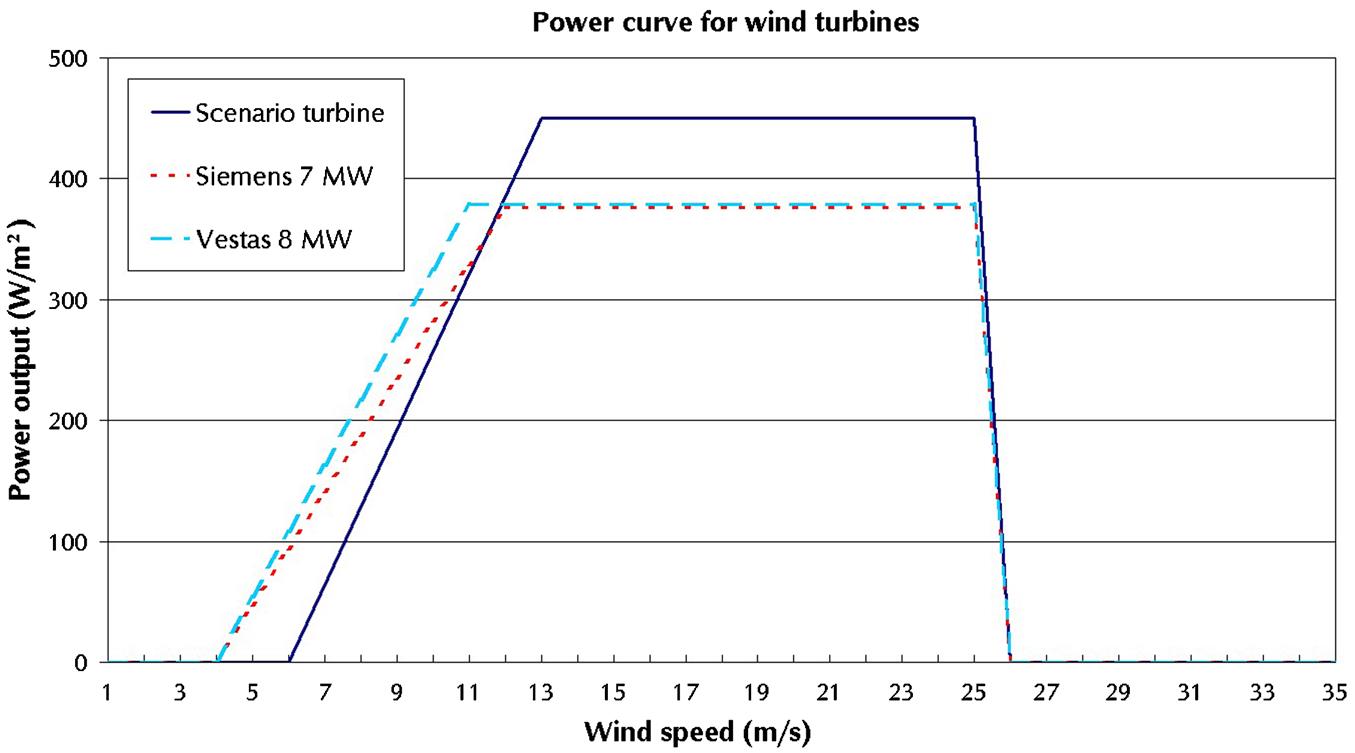
During the late 1970s, efforts were directed at several wind technologies: vertical axis machines in the United States and Canada, megawatt-size one- and two-bladed horizontal axis machines in the United States and Germany, and rotors with tip-vanes in the Netherlands. Yet, the winning technology was the Danish three-bladed, horizontal axis machine, starting in 1975 at a small unit size of 25–50 kW. The reason for this was primarily that the initial design was a scaled-down version of the 1957 fixed-pitch 200 kW Gedser turbine with blade stall control, gearbox, and asynchronous generator, i.e., an already proven design, and that further development was for a long time taken in very small, safe enlargement steps, gradually reaching megawatt size, rather than facing the problems of a totally new design in one jump (cf. Figs. 6.23 and 6.24).
Scaling up means controlling the most critical components, such as the rotor blades, which must be able to survive the forces on long pieces of suitable material, experiencing wind loads with gust effects that can cause the blades to bend in different directions and exert large forces on the fastening point of the blades. In addition, pitch change of blade angles has been introduced and thereby new options for operation or shutdown in high winds. Current production of megawatt units spreads over a number of different design principles. Interesting questions are being asked about whether there is a limit to the length of blades. Considerations should include the blade operating life aimed for. Currently, it is designed to be equal to the lifetime of the entire turbine, in contrast to faster rotating helicopter rotor blades, which have to be replaced at short intervals during the aircraft lifetime.
Figure 6.23 shows that a major technology shift, increased blade length, took place around 1994. In Denmark, this reflects the transition from mainly individually placed wind turbines to utility-owned wind parks or wind farms. Individual owners, mainly farmers, had carried the development of wind-power technology to maturity with essentially no help from established utility companies. This may be the chief explanation for the early high penetration of wind energy in Denmark. Later development has been dominated by utility wind parks, onshore or offshore. Utility privatization has caused some political fluctuation in the further development. Figure 6.24 indicates that a significant increase in turbine rated power has appeared since 1998, but that the average production per meter swept has declined since 2005. Earlier machines, placed at favorable land sites, were most often optimized to give the maximum energy production over the year, but the new ones at first had lower annual production (because the wind conditions offshore were underestimated) and then on purpose lowered annual output in order to get more operating hours over the year (due in part to economically unfavorable power exchange conditions set by the Norwegian hydro storage operators).
Design optimization is not a trivial matter, as it involves considerations of average energy produced, number of hours operating, and maximum loads exerted upon the structure. Figure 6.26 shows the calculated power output at onshore and offshore locations in the inner Danish region, indicating that the imposed power ceiling is reached more often offshore. This situation would occur more frequently at offshore locations in the North Sea, such as that of the Hornsrev wind farms, and new turbine designs have therefore increased the generator capacity relative to the area swept by the turbine. The choice of blade profiles, the sizing of the power generator, and the regulation strategies used in current megawatt-size machines have been improved to obtain better performance at Danish offshore sites as well as at many markets that have opened for offshore wind around the world. Danish wind technology has been transferred to companies in other parts of the world, such as the currently largest market in China, or the Danish company that has been sold to foreign investors (such as Siemens). Much easier to deal with is the advantage of a lower hub height (entailing lower cost) in the offshore locations with rapidly rising wind profiles, relative to the land sites where a high tower can diminish the negative effect of surface roughness (trees, buildings, etc.). Today, turbines are offered with a broad choice of hub height.
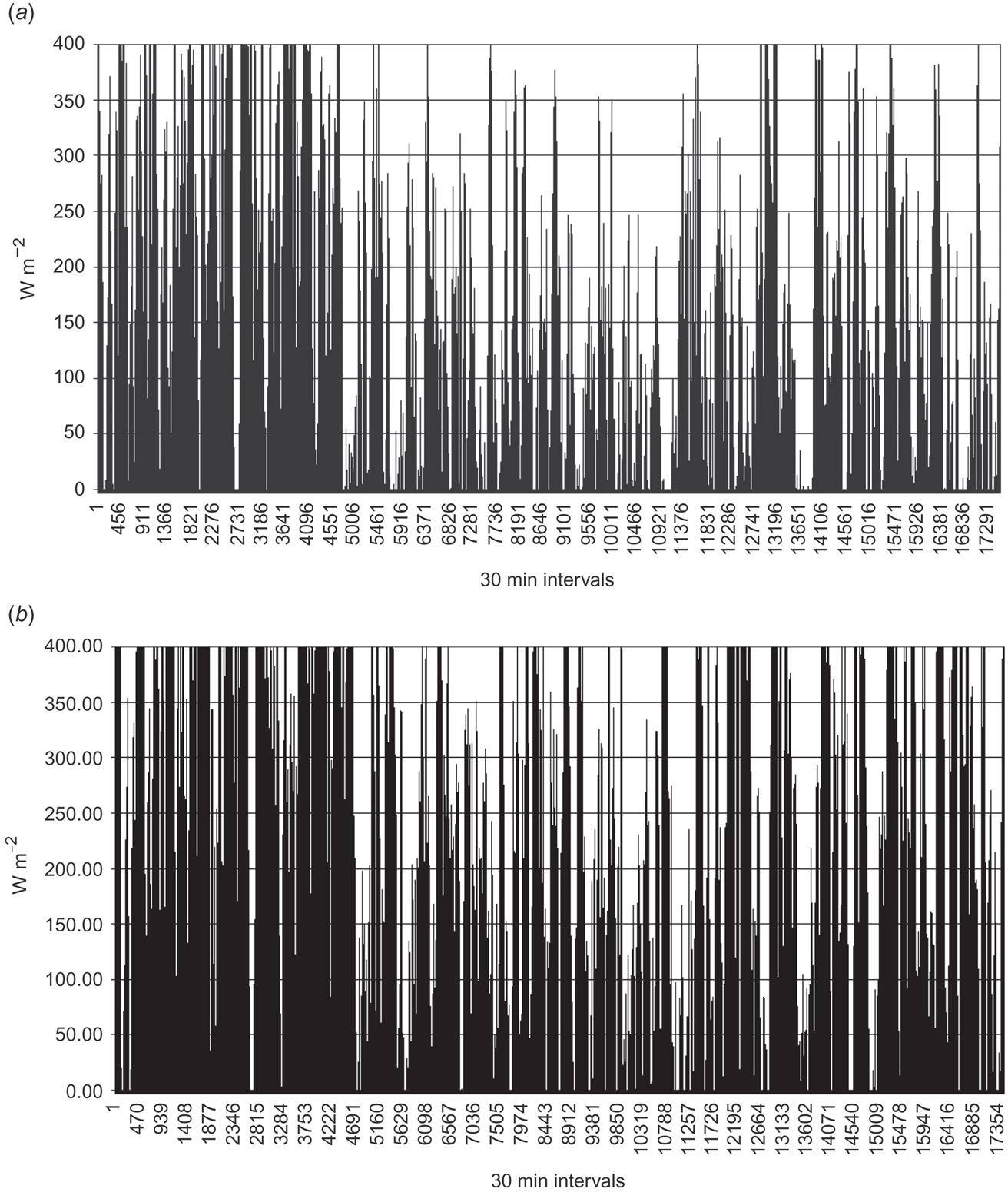
The model calculation assumes a constant Cp at high wind speeds, up to a maximum wind speed of 25 m s−1, where the turbine is brought to a stop. This can produce an inconvenient stop-go effect for large wind parks, where a large chunk of capacity can appear or disappear over very short time intervals. This is remedied by introducing a softer shutdown at high wind speeds, in such a way that some turbines in a wind farm are allowed to produce power at higher wind speeds for a while (Siemens, 2016). Another issue is that wind turbine manufacturers like to offer the same set of turbines for use throughout the global markets, rather than accepting that different wind-speed regimes invite the use of turbines tailored to the site-specific conditions (cf. the example given in Figs. 6.27 and 6.28, for the 2 MW turbine considered below). This is not easy to accomplish, as the optimization would involve using different wind blade profiles in different locations.
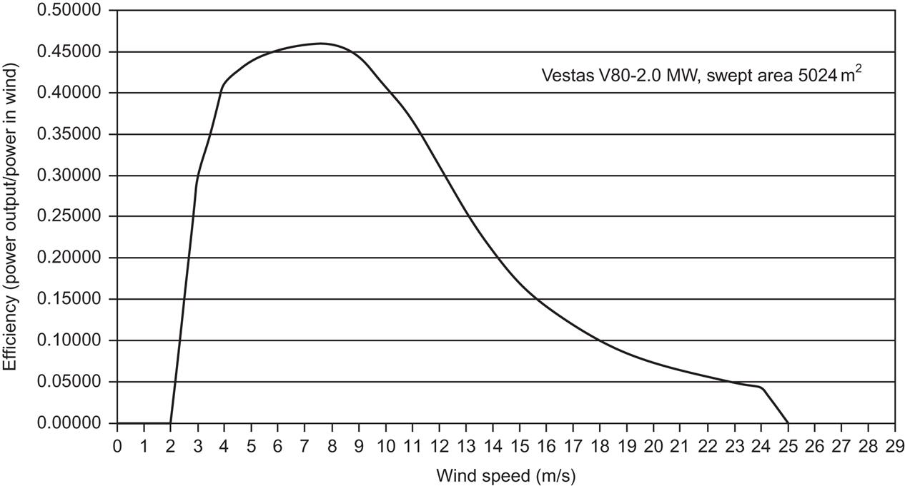
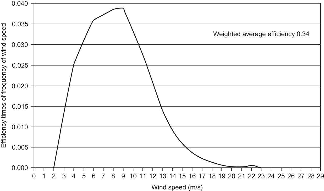
Table 6.6 shows an economic breakdown for a year-2000 vintage 2 MW turbine. There are, of course, variations of grid connection costs depending on location, and variations in the cost of the electric energy produced depending on financing conditions and the actual average power production at the location of the turbines. Theoretical details of payments occurring at different times and of interest rates are discussed in Chapter 7. Current costs are sometimes difficult to assess, as the price information furnished by the wind turbine manufacturers until about 2002 has been discontinued and sales revenues and conditions are often confidential. Some independent consultants try to obtain such information and sell it (to competitor companies) at high prices, and the remaining sources of information are primarily government-owned power utilities, although even they often give only summary information. Recent Chinese purchases of wind farms have been quoted as involving average capital costs of 1.6 (2015-)€/Wrated, giving a power cost of 0.094 (2015-)€/kWh when assuming an interest rate of 8% per year and a depreciation time (“lifetime”) of about 20 years (Tang and Popp, 2016). The capacity factor of Chinese wind farms is around 25%. For a recent Danish offshore wind farm with over a year’s operating experience (“Anholt-1”), the average capacity factor of 48% leads to a power price under standard assumptions of around 0.08 (2015-)€/kWh, despite a higher capital cost of 3.5 (2015-)€/Wrated (4C Offshore Consultancy UK, 2016). As it is uncertain that if the grid connection costs at sea and on land are included in the project cost estimate, it has been increased by 20%. The assumed lifetime used in the power price estimate is 20 years (conservative as the manufacturer, Siemens, claims 25 years), operation and maintenance costs are taken as 20% of the stated capital cost, and the depreciation rate used is 3% per year, which is the actual long-time interest rate in fixed prices in Europe for such projects.* The one project bidder (government-owned DONG) demanded a power delivery price of 0.14 €/kWh, clearly incorporating other costs such a premium for insurance against the contract’s penalty for cost and delivery time overruns (Danish Energy Agency, 2010), but it was accepted by a government in the process of fattening DONG for privatization sale. The bidding price for the newest Danish offshore wind park (“Hornsrev-3”) is closer to the estimate made here (0.10 €/kWh; Vattenfall, 2016). The park has forty-nine 8 MW Vestas turbines and a project capital cost of 2.5 (2015-)€/Wrated (4C Offshore Consultancy UK, 2016). The International Energy Agency quotes project costs for land-based wind farms across the world as being in the range of 1 to 2 (2014-)€/Wrated (IEA, 2015b).
Table 6.6
Installation price and cost of energy produced (in year-2015 prices), for wind parks on land or offshore.
| Installed cost (2015 €/Wrated) | Onshore | Offshore |
| Danish wind power installations around year 2000 | ||
| Turbines | 1.04 | 1.04 |
| Foundations | 0.08 | 0.47 |
| Grid connectiona | 0.20 | 0.36 |
| Engineering & administration | 0.05 | 0.05 |
| Land rights, access roads, facilities | 0.12 | 0.09 |
| Operation and maintenance (present value of 20 years’ cost) | 0.34 | 0.49 |
| Total capital cost including O&M (2015 €/Wrated) | 1.83 | 2.51 |
| Assumed power production | 2.6b | 3.8 |
| Cost of power produced (2015 €/kWh) | 0.047 | 0.045 |
| Chinese wind farms 2010–2015 (on- and offshore) | ||
| Project capital cost (2015 €/Wrated) | 1.6 | |
| Cost of power produced (2015 €/kWh) | 0.09 | |
| Danish offshore wind farms (2013–2016) | ||
| Project capital cost, Anholt-1 (2015 €/Wrated) | 3.5 | |
| Cost of power produced, Anholt-1 (2015 €/kWh) | 0.08 | |
| Project capital cost, Hornsrev 3 (2015 €/Wrated) | 2.5 | |
| IEA worldwide project cost examples (2015 €/Wrated) | 1 to 2 | |
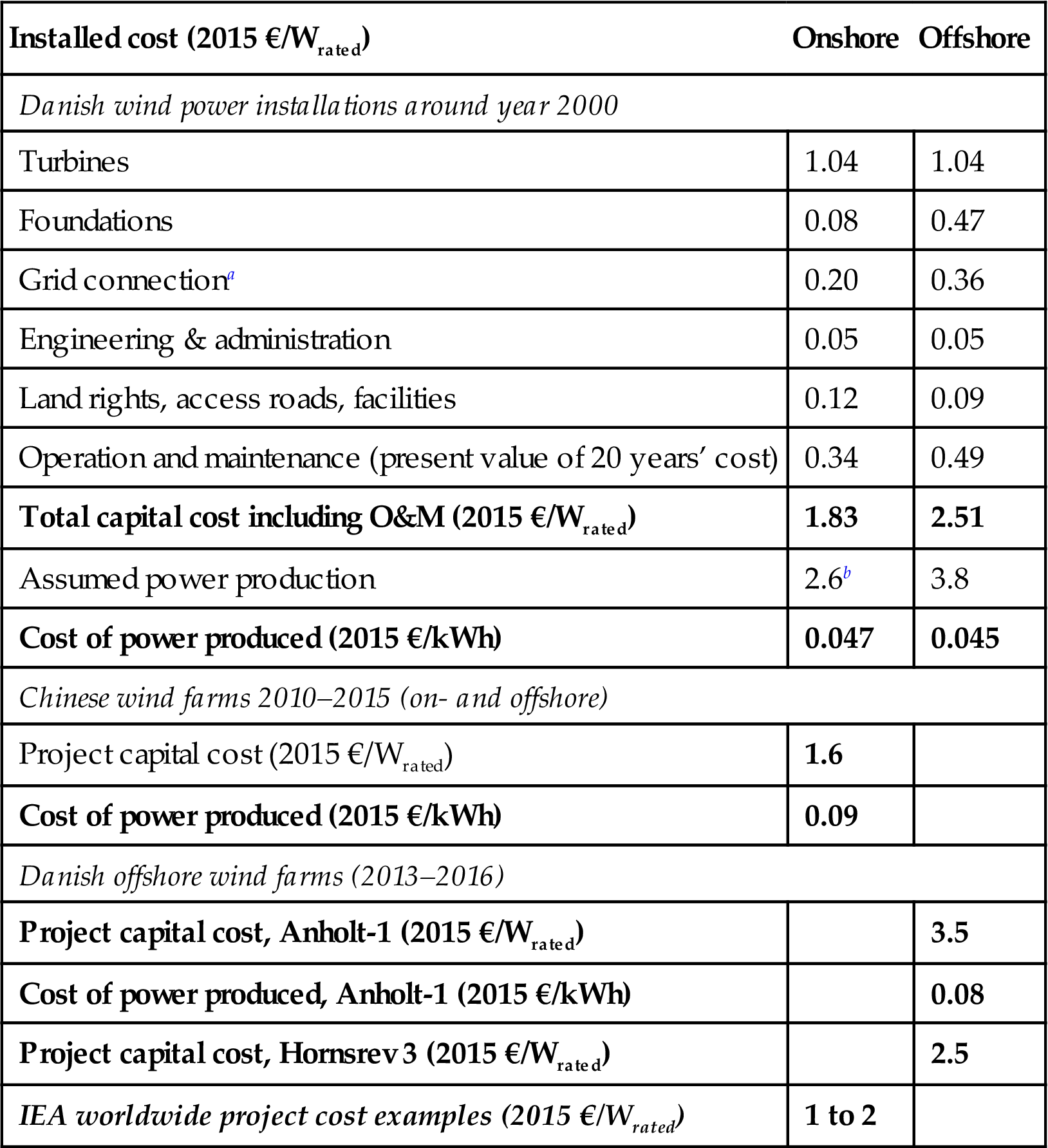
The detailed estimates with component breakdown have been made for Danish installations around year 2000, on the basis of price lists for 2 MW turbines, tender data and trend analysis (Danish wind turbine Price Lists and Overviews (1981–2002); Danish Energy Agency, 1999; European Commission, 2001). A depreciation time of 20 years and a real interest rate of 3% per year (8% for China) have been assumed, and prices are converted to year 2015 by use of deflators from OECD (2016). Thereafter follows total system cost and power production cost for recent installations in China (mainly onshore) and in Denmark (offshore), see text for sources and methods of estimation.
aThe Danish onshore grid connection costs are relatively low because of fairly short distances to grids of sufficient strength for most onshore Danish wind parks, but considerably higher for the offshore parks considered.
bOn the very best Danish inland locations, power production may approach 3.5 kWh/y/Wrated.
6.3.2.2 A new method for estimating offshore wind-power production
Because meteorological measuring stations are mostly placed on land, estimation of potential production from offshore sites is more difficult and has been unreliable in predicting the precise advantage of the more consistent and higher wind speeds known to prevail over the oceans. The new method for offshore wind-power prediction presented here (Sørensen, 2008a) is based on sweeping microwave radar (scatterometer) measurements by satellite, which provide radar wind data from reflections by the sea surface or airborne water particles over the sea surface. The original purpose of these satellite missions was quite different: to explore sea–atmosphere interactions important for climate modeling (Chelton et al., 2004).
Current offshore wind-power extraction typically involves propeller-type turbines with hub heights up to about 100 m above sea level and placed on foundations at a water depth of up to 50 m. During the last decade, satellite-based microwave scatterometer measurements of the effects of wind stresses on ocean surfaces have reached continuous, global coverage and improved accuracy in deriving near-surface wind speeds and directions from the radar reflection signals received at the satellite. The Seawinds instrument on the QuickSCAT satellite has provided such data since mid-1999 (NCAR, 2006). The sweeping pencil beams of microwave radiation emitted from the satellite have a frequency of 13.4×10⁹ s−1, corresponding to a wavelength of 0.022 m. This frequency lies in a band known for the smallness of atmospheric attenuation, allowing a simplified subtraction of such effects en route from, and back to, the satellite (Freilich, 1997).
The footprint of each pencil beam from the spinning parabolic antenna of the Seawinds system has an approximately 30 km×35 km elliptical area at the ocean surface. From a volume with this area and a certain height, the satellite receives a reflected radar signal. In fact, there are two transmitters and receivers operating at different azimuth angles, offering two looks at the same ocean area at short time intervals, thereby allowing an over-determination of wind velocities that is used to eliminate ambiguities in the directional solutions inherent in the algorithms used and to improve accuracy.
Conventionally, the reflections from the ocean surfaces are considered to arise from wind-generated capillary ripples on top of wave patterns, as well as from the wave surface and ocean surfaces in general. Capillary waves may be defined (see section 2.5.3) as those with wavelengths under some 0.02 m, i.e., with wavelength lower than, or similar to, that of the microwave beam used. However, additional sources of reflection may be whitecaps and water spray particles, which are often fairly abundant at heights up to around 20 m above the sea surface, but radiation at the beam frequency used would be fairly insensitive (Ulaby et al., 1981) to water particles much smaller than 0.01 m. Of the sources mentioned, the capillary waves are most directly linked to instantaneous wind stress, whereas gravity waves represent accumulated wind influence over periods that may involve many hours or even days, as evidenced by waves persisting long after the wind has quieted down. Like all moving sources, ocean currents induce a Doppler shift, unrelated to wind, in the microwave radar reflections. Rain will, depending on its intensity, blur the radar signal en route to or from the satellite, and it is customary to eliminate, or use models to correct, wind measurements affected by strong rain (Marzano et al., 2000; Milliff et al., 2004).
Because the backscattered signal averages over all of the mentioned processes within a volume equal to the kilometer-sized footprint times a height of some meters, one cannot identify a single type of reflection process as the source, but one does note a high sensitivity to the combined expressions of near-surface winds, implying that the wind vector extracted by use of the radar equation may have interesting applications.
Going from the wind speeds near the ocean surface to the productivity of megawatt wind turbines involves two additional calculations. One is to determine the height profile of the wind speeds and the other is to fold the wind-speed data with the conversion characteristics of a typical wind turbine. The height profile is that of a flow over a surface of a certain level of roughness. It may be described by the Monin-Obukhov relations (cf. section 3.2.1), which are derived from classical fluid dynamics and contain two parameters: the friction velocity of the air (which has as its dimension length, the square of which equals the surface wind stress over the air density) and a second parameter describing the stability of the air. The air-stability parameter more precisely describes the transport of heat across a unit area in the atmosphere. If this transport is zero, the atmosphere is said to be stable and, in that case, the height dependence of wind speeds is a simple logarithmic scaling law.
To estimate power production from wind turbines, it is customary to scale wind speeds to the turbine hub height by using the scaling law for a stable atmosphere, because the error is considered low due to insensitivity at both low and high wind speeds. The output from a typical propeller-type horizontal-axis wind turbine is zero for wind speeds below a threshold (say 5 ms−1), then rises to a maximum (at about 12 ms−1 wind speed), and stays there at higher wind speeds, until the turbine is shut down for safety reasons at high wind speeds (say above 25 ms−1).
Monthly year-2000 6-hour satellite scatterometer data downloaded from NCAR (2006) were uniformly scaled (by 1.3 for the illustrations presented here) and converted to wind turbine outputs by a power curve linearly rising from 0 to 450 Wm−2 between 5 ms−1 and 12 ms−1, staying at 450 Wm−1 until 25 ms−1 and then dropping to zero again. The roughness parameter used in the scaling law for the Dutch offshore site (see Fig. 6.29) is 0.0001 m. Monthly and annual average values were placed on a geographical grid of 0.5°-resolution on both axes and displayed using the Mollweide projection of the Earth in order that the areas with a given wind potential are faithfully represented (at the expense of a variable vertical-line distortion), and thus can be simply added or integrated. For the plots including wind direction (such as Fig. 6.31), a Mercator projection was used in order to achieve some similarity to conventional wind rose plots. Wind directions are not used in the potential power production calculations, assuming wind turbines with perfect yaw. This assumption is fulfilled in praxis, as any yawing adjustment to a new wind direction can be achieved in at most a few minutes by present-generation, large wind turbines.
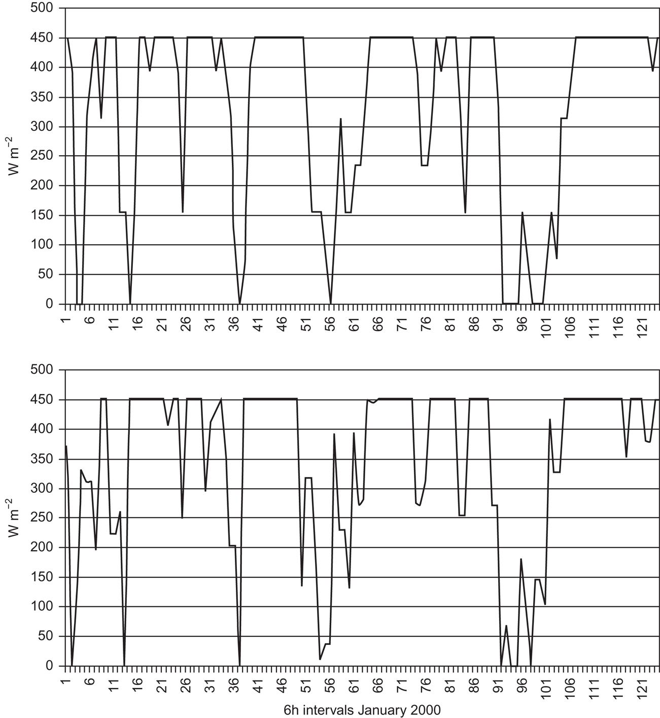
Figure 6.29 compares a January 2000 time-series of wind turbine outputs calculated from the scatterometer satellite data by the methods described above with outputs calculated from measured wind speeds for the same sequence of 6-hour intervals (Royal Dutch Meteorological Institute, 2006). The location is about 100 km offshore from the Dutch coast, at one of the few offshore locations where data are available at a height suitable for wind- power exploitation (74 m above the sea). The wind-speed scaling factor that makes the satellite data reproduce the total power production over the period derived from the measured wind speeds is 1.3. The 6-hour variations are reproduced very well by the proposed methodology.
While no other publicly available data that would allow similar direct comparison were found, the 1995 data from measurements performed as a prelude to the installation of Danish offshore wind farms are shown in Fig. 6.26. They have been compared to the predictions calculated from the year-2000 satellite data (Sørensen, 2008a). There is, of course, no detailed similarity between passages of weather fronts during a given calendar period in different years, but the overall picture of variability is similar, and the wind-speed scaling factor of 1.3 again reproduces the accumulated power production with an accuracy that suggests that satellite-based predictions using this scaling factor may be used generally for the identification of suitable sites for offshore wind installations.
The spatial resolution of the primary extracted scatterometer winds (Freilich, 1997) is roughly 25 km. Due to the intermittent passage of the satellite over a given location, these data have been blended with calculated wind speeds from general circulation models adapted to measured wind data on land (Kalnay et al., 1996; Milliff et al., 1999), in such a way that high-frequency variability from the scatterometer data is retained, while circulation model data are used for interpolation between satellite sweeps over a given location (the 1800-km-wide QuickSCAT sweeps take 101 minutes and a given location is measured at about 12-hour intervals). The resulting 6-hour data thus have high-quality input at each second time step, but only over water. For land sites, the radar reflections may come from a multitude of sources and the satellite data cannot easily be used to estimate wind speeds.
The blended data are presented on a grid of 0.5°×0.5°, combining the scatterometer swath resolution approaching 25 km with the results from the general circulation model, which, if used alone, would have an output resolution of the order of 250 km (for an input integration-step grid with 0.5°=56 km latitude grid-sides and for longitudinal grid-sides multiplied by the cosine of the latitude). For locations on land, the circulation model data are clearly unsuited for specific placement of wind turbines, but may give a fair indication of the wind potential of an extended region (cf. preceding section). The ocean and near-shore (from the sea side) blended data, on the other hand, offer a clear improvement over any existing method of estimating wind-power potential at these locations. Because of the finite grid size used in presenting the blended data, some blended data points along a given shoreline (on both land and water sides) could represent circulation-model calculations of low resolution rather than the high-resolution scatterometer readings. The offshore location used in Fig. 6.29 is sufficiently far from land to exclude any such problems.
Having established a scaling factor close to 1.3 in going from the primary scatterometer data to a height of 74 m over the sea surface, one can use the Monin-Obukhov relations to determine the average effective height z1 associated with the scatterometer data, a quantity that is otherwise not easy to assess, because the wind extraction method used in analyzing scatterometer data involves a search for the best solution under assumptions of simple stochastic distributions for the backscattered rays and without considering a particular height (Freilich, 1997). To estimate z1, one may use the logarithmic scaling law describing stable atmospheric situations,
where v1 and v2 are wind speeds at heights z1 and z2, log is the natural logarithm, and z0 the roughness length for the ocean surface, (3.24), related to the friction velocity and, as stated, being about 0.0001 m for the Dutch site (Royal Dutch Meteorological Institute, 2006). Because the Dutch measurements include this estimate of the roughness length z0 at the particular offshore location, the scaling law for a neutral atmosphere given above contains just one remaining unknown quantity, the reference height, which is then found to be 3 m (representing the height over the average sea surface that the scatterometer winds on average pertain to). This estimate is considered more accurate than one based upon speculations about the particular scattering objects involved, because it is based on long-term averages of a power calculation sensitive only to the most common mid-size wind speeds.
The 6-hour time-series constructed from the satellite data may be used to assess the variability of wind-power with time and location, and hence, for example, any need for inter-regional power trading or for establishing energy stores (Sørensen, 2008c). Short-term fluctuations (under 1 hour) are immediately smoothed by dispersing wind turbine locations over a few hundred kilometers, but smoothing over longer periods requires power transmission between regions of different weather (and hence wind) regimes, implying distances of some 500 km or more. In addition to determining full time-series, averages over time are taken, because they can be used to assess wind-power production potentials over periods deemed important, from weeks to years.
Decisions to build wind turbine parks are often taken based on expected average annual production, and a global map of production potentials is shown in Fig. 6.30. As stated above, the accuracy over land is low and values shown should be taken as indicative only for large regions. One would expect scaling factors for translating the scatterometer data to potential wind speeds at turbine hub heights to vary rapidly with location. Comparing the new blended data with the 1998 re-analysis data, one finds no compelling reasons to alter the 1.3 scaling-factor value over land in estimating regional wind-power. One might have suspected that larger roughness would lead to a larger scaling factor, but the blended data for continental locations are dominated by the circulation-model data, and the “effective height” associated with them (for the lowest model level) is likely to be considerably larger than the 3 m found for the ocean data.
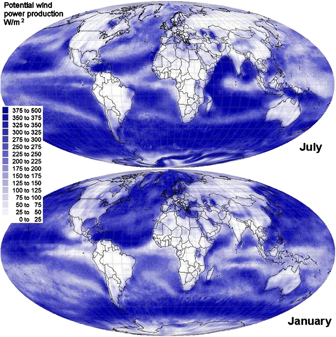
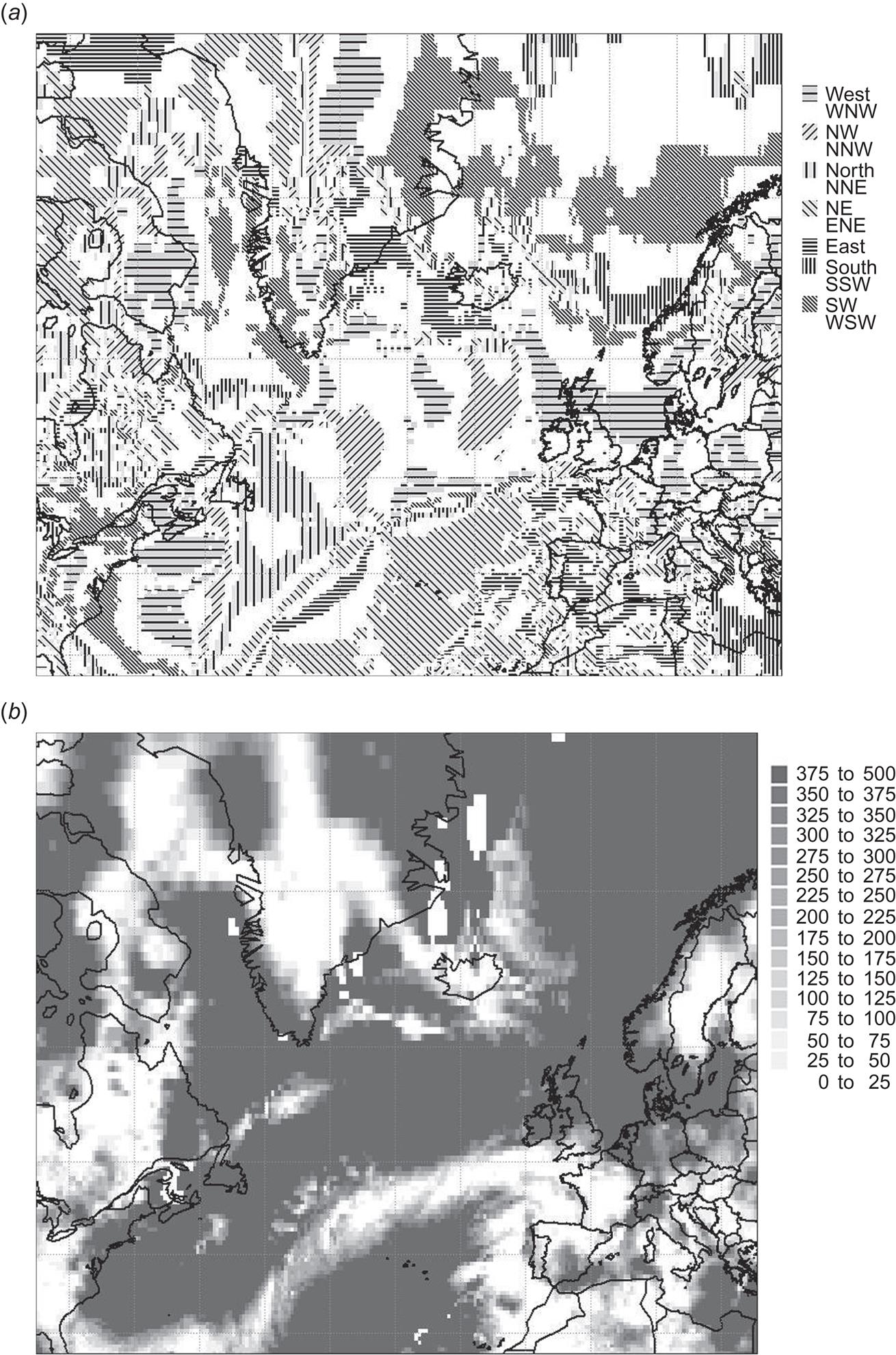
For offshore locations, the spatial resolution is quite acceptable due to the absence of abrupt roughness variations. Variations in power production over the year are considered in planning offshore wind parks. Averages similar to Fig. 6.30, but for the wind speeds rather than turbine output power, have been published (Jet Propulsion Laboratory, 2007; Risien and Chelton, 2006), but they are not suited for wind turbine power estimates, due to the non-linear power curve that excludes deriving accurate average power levels from average wind speeds.
Figure 6.30 emphasizes, first, the huge advantage of producing wind-power over water, not only in mid-ocean locations but also at shore-regions of several continents. However, it also indicates that a number of coastal sites are less suitable, notably sites on the western side of continents near the Equator and on both sides of Equatorial sites south and southeast of the Asian continent. Closer inspection of shorelines farther away from the Equator shows notable differences in the generally large wind potentials, with a number of very-high-potential coastlines existing on all continents, but some of them not yet considered for energy exploitation. Of course, additional factors may influence suitability for constructing power facilities, such as whether the water depth increases more or less rapidly away from the shore. Further, a number of inland water systems stand out as highly suitable for wind-power, including the Great Lakes in North America, the Baltic Sea and parts of the Mediterranean Sea in Europe, the Caspian and Aral Seas near the Europe-Asia border, and Lake Victoria in Africa.
To address wind turbine operational issues, such as the need for power exchange between regions or storage (Sørensen, 2008c, 2015), the blended data offer 6-hour calculations of both the expected power output and the direction from which the turbine must accept winds. Figure 6.31 shows an example of such a sequence of 6-hour data, for a region in the North Atlantic Ocean. The data are for January 26. There is a storm blowing from the southwest at the Florida coast and turning to the west as it reaches the British Isles and Scandinavia. These countries and Germany are seen to be capable of producing large amounts of power, while France, Central Europe, and the Mediterranean countries (except for a few south-facing coasts) need to import power or use alternative solutions. Such examples indicate some modes of application made possible by the quality of data derived from the scatterometer satellite measurements.
6.3.3 Food production
The general model used in the scenario model to describe the biomass sector is shown in Fig. 6.32. It is a refinement of a model developed earlier (Sørensen et al., 1994; Sørensen, 1994). Each part of the model is discussed below, and numerical assumptions are stated.