
Energy transmission and storage
Abstract
Energy transmission options are discussed, with heat, electric power or fuel as the carrier of energy. Energy storage and retrieval technologies are surveyed, covering heat capacity, latent heat and chemical transformation stores of heat, and for electricity storage pumped hydro, flywheels, compressed gas stores, battery stores and hydrogen underground stores.
Keywords
Transmission of energy; Heat storage; High-quality energy storage; Hydro stores; Compressed gas stores; Hydrogen stores; Battery stores
5.1 Energy transmission
Transport of energy may, as traditionally, be in the form of transportation of fuels to the site of conversion. With regard to renewable energy resources, such transport is useful for biomass-derived energy, either by direct movement of the biological materials themselves or by movement after their conversion into biofuels (cf. section 4.6), which may be more convenient to move. For most other types of renewable energy, the resource itself cannot be “moved” (possible exceptions may exist, such as diverting a river flow to the place of hydropower utilization). Instead, an initial conversion process may be performed, and the emerging energy form may be transmitted to the load areas, where it may be used directly or subjected to a second conversion process before delivery to the actual users.
Like fuels (which represent chemical energy), heat and mechanical and possibly electrical energy may be stored, and the storage “containers” may be transported. Alternatively, energy may be transmitted through a suitable transmission system, which may be a pipeline (for heat, fuels, and certain types of mechanical energy, such as pressure or kinetic energy of a gas or a fluid), electric lines (for electricity), or a radiant transmission system (for heat or electricity).
Energy transmission is used not only to deliver energy from the sites of generation (such as where the renewable resources are) to the dominant sites of energy use, but also to deal with temporal mismatch between (renewable) energy generation and variations in demand. Therefore, energy transmission and energy storage may supplement each other. Some demands may be displaceable, while others are time-sensitive. The latter often display a systematic variation over the hours of the day and over the seasons. This may be taken advantage of by long-distance transmission of energy across time zones (east–west).
5.1.1 Heat transmission
5.1.1.1 District heating lines
Most heating systems involve the transport of sensible heat in a fluid or gas (such as water or air) through pipes or channels. Examples are the solar heating system illustrated in Fig. 4.84, the heat pump illustrated in Fig. 4.6, and the geothermal heating plants illustrated in Fig. 4.9. Solar heating systems and heat pumps may be used in a decentralized manner, with an individual system providing heat for a single building, but they may also be used on a community scale, with one installation providing heat for a building block, a factory complex, a whole village, or a city of a certain size. Many combined heat and power (CHP) systems involve heat transmission through distances of 10–50 km (decentralized and centralized CHP plants). In some regions, pure heating plants are attached to a district-heating grid.
If a hot fluid or gas is produced at the central conversion plant, transmission may be accomplished by pumping the fluid or gas through a pipeline to the load points. The pipeline may be placed underground and the tubing insulated in order to reduce conduction and convection of heat away from the pipe. If the temperature of the surrounding medium can be regarded as approximately constant, equal to Tref, the variation in fluid (or gas) temperature Tfluid(x) along the transmission line (with the path-length co-ordinate denoted x) can be evaluated by the same expression (4.36) used in the simple description of a heat exchanger in section 4.2.3. Temperature variations across the inside area of the pipe perpendicular to the streamwise direction are not considered.
The rate of heat loss from the pipe section between the distances x and (x+dx) is then of the form
(5.1)
where h′ for a cylindrical insulated pipe of inner and outer radii r1 and r2 is related to the heat transfer coefficient λpipe [conductivity plus convection terms, cf. (3.34)] by
Upon integration from the beginning of the transmission pipe, x=x1, (5.1) gives, in analogy to (4.36),
(5.2)
where Jm is the mass flow rate and ![]() is the fluid (or gas) heat capacity. The total rate of heat loss due to the temperature gradient between the fluid in the pipe and the surroundings is obtained by integrating (5.1) from x1 to the end of the line, x2,
is the fluid (or gas) heat capacity. The total rate of heat loss due to the temperature gradient between the fluid in the pipe and the surroundings is obtained by integrating (5.1) from x1 to the end of the line, x2,
The relative loss of heat supplied to the pipeline, along the entire transmission line, is then
(5.3)
 (5.3)
(5.3)
provided that the heat entering the pipe, E, is measured relative to a reservoir of temperature Tref.
The total transmission loss will be larger than (5.3) because of friction in the pipe. The distribution of flow velocity, v, over the pipe’s inside cross-section depends on the roughness of the inner walls (v being zero at the wall), and the velocity profile generally depends on the magnitude of the velocity (say at the centerline). Extensive literature exists on the flow in pipes (see, for example, Grimson, 1971). The net result is that additional energy must be provided in order to make up for the pipe losses. For an incompressible fluid moving in a horizontal pipe of constant dimensions, flow continuity demands that the velocity field be constant along the pipeline, and, in this case, the friction can be described by a uniformly decreasing pressure in the streamwise direction. A pump must provide the energy flux necessary to compensate for the pressure loss,
where A is the area of the inner pipe cross-section and ΔP is the total pressure drop along the pipeline.
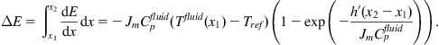
Transmission lines presently in use for city district heating have average heat losses of 10%–15%, depending on insulation thickness (see, for example, WEC, 1991). The pump energy added is in the form of high-quality mechanical work, but with proper dimensioning of the tubes it may be kept to a small fraction of the heat energy transmitted. This energy is converted into heat by frictional dissipation, and some of the heat may actually be credited to the heat transmission. Maximum heat transmission distances currently considered economical are around 30 km, with the possible exception of some geothermal installations. Figure 5.1 shows an integrated design that allows much easier installation than earlier pipes with separate insulation. In countries with a high penetration of combined heat and power production, such as Denmark, a heat storage facility holding some 10 h of heat load is sometimes added to each plant, in order that the (fuel-based) plant does not have to generate more electric power than needed, say, at night, when the heating load is large (Danish Energy Agency, 1993).
5.1.1.2 Heat pipes
A special heat transmission problem arises where very large amounts of heat have to be delivered to, or removed from, a small region, for example, in connection with highly concentrating solar energy collectors. Such heat transfer may be accomplished by a heat pipe, a device described in section 4.2.1 in relation to thermionic generators.
5.1.2 Power transmission
5.1.2.1 Normal conducting lines
At present, electric current is transmitted in major utility grids, as well as distributed locally to each load site by means of conducting wires. Electricity use is dominated by alternating current (AC), as far as utility networks are concerned, and most transmission over distances up to a few hundred kilometers is by AC. For transmission over longer distances (e.g., by ocean cables), conversion to direct current (DC) before transmission and back to AC after transmission is common. A new 1.1 MV land DC transmission line in China connects Guquan with Changqi some 3000 km apart (Anonymous, 2016). In densely populated areas, increasing use of cables buried in the ground (with appropriate electric insulation) is often seen but also overhead lines suspended in the air between masts, without electrical insulation around the wires, are still common in areas where the visual impact is deemed acceptable (such as for the Chinese link). Insulating connections are provided at the tower fastening points, but otherwise the low electric conductivity of air is counted on. This implies that the losses will comprise conduction losses depending on the instantaneous state of the air (the “weather situation”), in addition to the ohmic losses connected with the resistance R of the wire itself, Ehea=RI2, with I being the current. The leak current between the elevated wire and the ground depends on the potential difference as well as on the integrated resistivity (cf. section 3.4.5), such that the larger the voltage, the further the wires must be placed from the ground.
Averaged over different meteorological conditions, the losses in a standard AC overhead transmission line (138–400 kV, at an elevation of 15–40 m) are currently a little under 1% per 100 km of transmission (Hammond et al., 1973), but the overall transmission losses of utility networks, including the finely branched distribution networks in the load areas, may for many older, existing grids amount to 12%–15% of the power production for a grid extending over a land area of about 104 km2 (Blegaa et al., 1976). Around year 2000, losses were down to 5%–6% for the best systems installed, and they are expected to reach 2%–3% for the currently best technologies (Kuemmel et al., 1997). This loss is calculated relative to the total production of electricity at the power plants attached to the common grid, and thus includes certain in-plant and transformer losses. The numbers also represent annual averages for a power utility system occasionally exchanging power with other utility systems through interconnecting transmission lines, which may involve transmission distances much longer than the linear extent of the load area being serviced by the single utility system in question.
The trend is to replace overhead lines with underground cables, primarily for visual and environmental reasons. This has already happened for the distribution lines in Europe and is increasingly also being required for transmission lines. In Japan and the United States, overhead lines are still common.
Underground transmission and distribution lines range from simple coaxial cables to more sophisticated constructions insulated by compressed gas. Several transoceanic cables (up to 1000 km) have been installed in Scandinavia in order to bring the potentially large surpluses of hydropower production to the European continent. The losses through these high-voltage (up to 1000 kV) DC lines are under 0.4% per 100 km, to which should be added the 1%–2% transmission loss occurring at the thyristor converters on shore that transform AC into DC and vice versa (Chapter 19 in IPCC, 1996). The cost of these low-loss lines is currently approaching that of conventional AC underwater cables (about 2 euro kW−1 km−1; Meibom et al., 1997, 1999; Wizelius, 1998).
One factor influencing the performance of underground transmission lines is the slowness of heat transport in most soils. In order to maintain the temperature within the limits required by the materials used, active cooling of the cable could be introduced, particularly if large amounts of power have to be transmitted. For example, the cable may be cooled to 77 K (liquid nitrogen temperature) by means of refrigerators spaced at intervals of about 10 km (cf. Hammond et al., 1973). This allows increased amounts of power to be transmitted in a given cable, but the overall losses are hardly reduced, since the reduced resistance in the conductors is probably outweighed by the energy spent on cooling. According to (4.22), the cooling efficiency is limited by a Carnot value of around 0.35, i.e., more than three units of work have to be supplied in order to remove one unit of heat at 77 K.
5.1.3 Offshore issues
The power from an offshore wind farm is transmitted to an onshore distribution hub by means of one or more undersea cables, the latter providing redundancy that, in the case of large farms, adds security against cable disruption or similar failures. Current offshore wind farms use AC cables of up to 150 kV (Eltra, 2003). New installations use cables carrying all three leads plus control wiring. In the interest of loss minimization for larger installations, it is expected that future systems may accept the higher cost of DC–AC conversion (on shore, the need for AC–DC conversion at sea depends on the generator type used), similar to the technology presently in use for many undersea cable connections between national grids (e.g., between Denmark and Norway or Sweden). Recent development of voltage source-based high-voltage DC control systems to replace the earlier thyristor-based technology promises better means of regulation of the interface of the DC link to the onshore AC system (Ackermann, 2002).
5.1.3.1 Superconducting lines
For DC transmission, ohmic losses may be completely eliminated by use of superconducting lines. A number of elements, alloys, and compounds become superconducting when cooled to a sufficiently low temperature. Physically, the onset of superconductivity is associated with the sudden appearance of an energy gap between the ground state, i.e., the overall state of the electrons, and any excited electron state (similar to the situation illustrated in Fig. 4.48, but for the entire system rather than for individual electrons). A current, i.e., a collective displacement (flow) of electrons, will not be able to excite the system away from the ground state unless the interaction is strong enough to overcome the energy gap. This implies that no mechanism is available for the transfer of energy from the current to other degrees of freedom, and thus the current will not lose any energy, which is equivalent to stating that the resistance is zero. In order for the electron system to remain in the ground state, the thermal energy spread must be smaller than the energy needed to cross the energy gap. This is the reason why superconductivity occurs only below a certain temperature, which may be quite low (e.g., 9 K for niobium, 18 K for niobium–tin, Nb3Sn). However, there are other mechanisms that in more complex compounds can prevent instability, thereby explaining the findings in recent years of materials that exhibit superconductivity at temperatures approaching ambient (Pines, 1994; Demler and Zhang, 1998).
For AC transmission, a superconducting line will not be loss-free, owing to excitations caused by the time variations of the electromagnetic field (cf. Hein, 1974), but the losses will be much smaller than for normal lines. It is estimated that the amount of power that can be transmitted through a single cable is in the gigawatt range. This figure is based on suggested designs, including the required refrigeration and thermal insulation components within overall dimensions of about 0.5 m (cable diameter). The power required for cooling, i.e., to compensate for heat flow into the cable, must be considered in calculating the total power losses in transmission.
For transmission over longer distances, it may, in any case, be an advantage to use direct current, despite the losses in the AC–DC and DC–AC conversions (a few percent, as discussed above). Intercontinental transmission using superconducting lines has been discussed by Nielsen and Sørensen (1996) and by Sørensen and Meibom (1998) (cf. scenario in section 6.7). The impetus for this is of course the location of some very promising renewable energy sites far from the areas of load. Examples are solar installations in the Sahara or other desert areas, or wind power installations at isolated rocky coastlines of northern Norway or in Siberian highlands.
Finally, radiant transmission of electrical energy may be mentioned. The technique for transmitting radiation and re-collecting the energy (or some part of it) is well developed for wavelengths near or above visible light. Examples are laser beams (stimulated atomic emission) and microwave beams (produced by accelerating charges in suitable antennas), ranging from the infrared to the wavelengths used for radio and other data transmission (e.g., between satellites and ground-based receivers). Large-scale transmission of energy in the form of microwave radiation has been proposed in connection with satellite solar power generation, but it is not currently considered practical. Short-distance transmission of signals, e.g., between computers and peripheral units, involves only minute transfers of energy and is already in widespread use.
5.1.4 Fuel transmission
Fuels like natural gas, biogas, hydrogen, and other energy-carrier gases may be transmitted through pipelines, at the expense of only a modest amount of pumping energy (at least for horizontal transfer). Pipeline oil transmission is also in abundant use. Intercontinental transport may alternatively use containers onboard ships for solid fuels, oil, compressed gases or liquefied gases. Similar containers are used for shorter-distance transport by rail or road. Higher energy densities may be attained by the energy storage devices discussed in section 5.2.2, such as metal hydrides or carbon nanotubes, e.g., for hydrogen transport. Lightweight container materials are, of course, preferable in order to reduce the cost of moving fuels by vessel, whether on land or at sea.
Current natural gas networks consist of plastic distribution lines operated at pressures of 0.103 to about 0.4 MPa and steel transmission lines operated at pressures of 5–8 MPa. With upgraded valves, some modern natural gas pipelines could be used for the transmission of hydrogen (Sørensen et al., 2001). Certain steel types may become brittle with time, as a result of hydrogen penetration into the material, and cracks may develop. It is believed that H2S impurities in the hydrogen stream increase the problem, but investigations of the steel types currently used for new pipelines indicate little probability of damage by hydrogen (Pöpperling et al., 1982; Kussmaul and Deimel, 1995).
Mechanical devices have been used to transfer mechanical energy over short distances, but mechanical connections with moving parts are not practical for distances of transfer that may be considered relevant for transmission lines. However, mechanical energy in forms like hydraulic pulses can be transmitted over longer distances in feasible ways, as, for example, mentioned in connection with wave energy conversion devices placed in open oceans (section 4.3.6).
5.2 Heat storage
Storage of energy allows adjustment to variations in energy demand, i.e., it provides a way of meeting a load with a time-dependence different from that of generation. For fuel-type energy, storage can help burn the fuel more efficiently, by avoiding situations where demand variations would otherwise require regulation of combustion rates beyond what is technically feasible or economic. For fluctuating renewable energy sources, storage helps make the energy systems as dependable as fuel-based systems.
The characteristics of an ideal energy storage system include availability for rapid access and versatility of the form in which energy from the store is delivered. Conversion of one type of stored energy (initial fuel) into another form of stored energy may be advantageous for utilization. For example, production of electricity in large fossil fuel or nuclear power plants may involve long start-up times that incur additional costs when used for load leveling, while pumped water storage allows delivery upon demand in less than a minute. The economic feasibility of energy storage depends on the relative fixed and variable costs of the different converter types and on the cost and availability of different fuels. Another example is a fuel-driven automobile, which operates at or near peak power only during short intervals of acceleration. If short-term storage is provided that can accumulate energy produced off-peak by the automobile engine and deliver the power for starting and acceleration, then the capacity rating of the primary engine may be greatly reduced.
In connection with renewable energy resources, most of which are intermittent and of a fluctuating power level, supplementing conversion by energy storage is essential if the actual demand is to be met at all times. The only alternative would seem to be fuel-based back-up conversion equipment, but this, of course, is just a kind of energy storage that in the long run may require fuels provided by conversion processes based on renewable primary energy sources.
5.2.1 Heat capacity storage
Heat capacity, or “sensible heat” storage, is accomplished by changing the temperature of a material without changing its phase or chemical composition. The amount of energy stored by heating a piece of material of mass m from temperature T0 to temperature T1 at constant pressure is
(5.4)
where cP is the specific heat capacity at constant pressure.
Energy storage at low temperatures is needed in renewable systems like solar absorbers delivering space heating, hot water, and eventually heat for cooking (up to 100°C). The actual heat storage devices may be of modest size, aiming at delivering heat during the night after a sunny day, or they may be somewhat larger, capable of meeting demand during a number of consecutive overcast days. Finally, the storage system may provide seasonal storage of heat, as required at high latitudes where seasonal variations in solar radiation are large, and, furthermore, heat loads are to some extent inversely correlated with the length of the day.
Another aspect of low-temperature heat storage (as well as of some other energy forms) is the amount of decentralization. Many solar absorption systems are conveniently placed on existing rooftops; that is, they are highly decentralized. A sensible heat store, however, typically loses heat from its container, insulated or not, in proportion to the surface area. The relative heat loss is smaller, the larger the store dimensions, and thus more centralized storage facilities, for example, of communal size, may prove superior to individual installations. This depends on an economic balance between the size advantage and the cost of additional heat transmission lines for connecting individual buildings to a central storage facility. One should also consider other advantages, such as the supply security offered by the common storage facility (which would be able to deliver heat, for instance, to a building with malfunctioning solar collectors).
5.2.2 Water storage
Heat energy intended for later use at temperatures below 100°C may be conveniently stored as hot water, owing to the high heat capacity of water (4180 J kg−1 K−1 or 4.18×10⁶ J m−3 K−1 at standard temperature and pressure), combined with the fairly low thermal conductivity of water (0.56 J m−1 s−1 K−1 at 0°C, rising to 0.68 J m−1 s−1 K−1 at 100°C).
Most space heating and hot water systems for individual buildings include a water storage tank, usually in the form of an insulated steel container with a capacity corresponding to less than a day’s hot water usage and often only a small fraction of a cold winter day’s space heating load. For a one-family dwelling, a 0.1-m3 tank is typical in Europe and the United States.
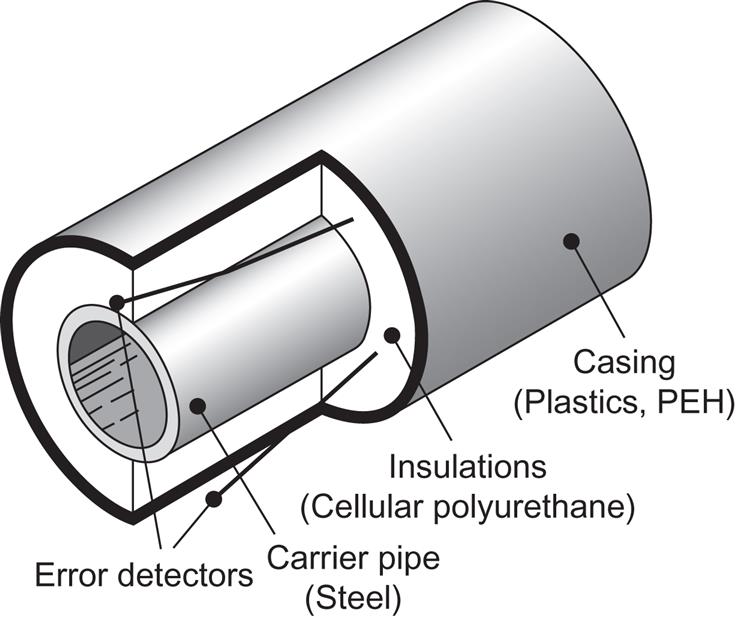
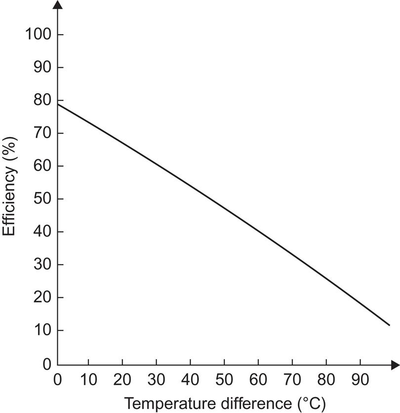
A steel hot water container may look like the one sketched in Fig. 5.2. It is cylindrical, with a height greater than the diameter, in order to make good temperature stratification possible, an important feature if the container is part of a solar heating system. A temperature difference of up to 50°C between the top and bottom water can be maintained, with substantial improvements (over 15%) in the performance of the solar collector heating system, because the conversion efficiency of the collector declines (see Fig. 5.3) with the temperature difference between the water coming into the collector and the ambient outdoor temperature (Koppen et al., 1979). Thus, the water from the cold lower part of the storage tank would be used as input to the solar collector circuit, and the heated water leaving the solar absorber would be delivered to a higher-temperature region of the storage tank, normally the top layer. The take-out from the storage tank to load (directly or through a heat exchanger) is also from the top of the tank, because the solar system will, in this case, be able to cover load over a longer period of the year (and possibly for the entire year). There is typically a minimum temperature required for the fluid carrying heat to the load areas, and during winter, the solar collector system may not always be able to raise the entire storage tank volume to a temperature above this threshold. Thus, temperature stratification in storage containers is often a helpful feature. The minimum load-input temperatures are around 45 °C–50°C for space heating through water-filled radiators and convectors, but only 25 °C–30°C for water-filled floor heating systems and air-based heating and ventilation duct systems.

For hot water provision for a single family, using solar collector systems with a few square meters of collectors (1 m2 in sunny climates, 3–5 m2 at high latitudes), a storage tank of around 0.3 m3 is sufficient for diurnal storage, while a larger tank is needed if consecutive days of zero solar heat absorption can be expected. For complete hot water and space heating solar systems, storage requirements can be quite substantial if load is to be met at all times and the solar radiation has a pronounced seasonal variation.
Most solar collector systems aiming at provision of both hot water and space heating for a single-family dwelling have a fairly small volume of storage and rely on auxiliary heat sources. This is the result of an economic trade-off due to the rapid reduction in solar collector gains with increasing coverage, that is, the energy supplied by the last square meter of collector added to the system becomes smaller and smaller as the total collector area increases. Of course, the gain is higher with increased storage for a fixed collector area over some range of system sizes, but the gain is very modest (see section 6.5.1).
For this reason, many solar space-heating systems only have diurnal storage (for example, a hot water storage). In order to avoid boiling, when the solar radiation level is high for a given day, the circulation from storage tank to collector is disconnected whenever the storage temperature is above some specified value (e.g., 80°C), and the collector becomes stagnant. This is usually no problem for simple collectors with one layer of glazing and black paint absorber, but for multilayered covers or selective-surface coating of the absorber, the stagnation temperatures are often too high and materials would be damaged before these temperatures were reached. Instead, the storage size may be increased to such a value that continuous circulation of water from storage through collectors can be maintained during sunny days without violating maximum storage temperature requirements at any time during the year. If the solar collector is so efficient that it still has a net gain above 100°C (such as the one shown in Fig. 5.3), this heat gain must be balanced by heat losses from piping and from the storage itself, or the store must be large enough for the accumulated temperature rise during the most sunny periods of the year to be acceptable. In high-latitude climatic regions, this can be achieved with a few square meters of water storage, for collector areas up to about 50 m2.
Larger amounts of storage may be useful if the winter is generally sunny, but a few consecutive days of poor solar radiation do occur from time to time. For example, the experimental house in Regina, Saskatchewan (Besant et al., 1979) is superinsulated and is designed to derive 33% of its heating load from passive gains of south-facing windows, 55% from activities in the house (body heat, electric appliances), and the remaining 12% from high-efficiency (evacuated tube) solar collectors. The collector area is 18 m2 and there is a 13 m3 water storage tank. On a January day with outdoor temperatures between –25°C (afternoon) and –30°C (early morning), about half the building’s heat loss is replaced by indirect gains, and the other half (about 160 MJ d−1) must be drawn from the store, in order to maintain an indoor temperature of 21°C (although the temperature is allowed to drop to 17°C between midnight and 0700 h). On sunny January days, the amount of energy drawn from storage is reduced to about 70 MJ d−1. Since overcast periods of much over a week occur very rarely, the storage size is such that 100% coverage can be expected, from indirect and direct solar sources, in most years.
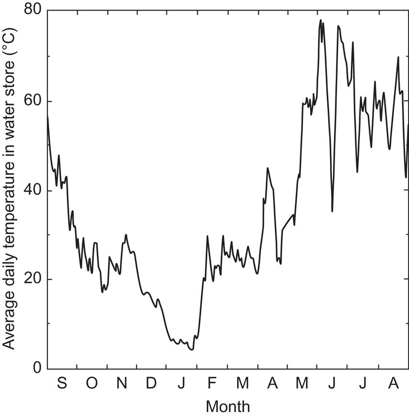
The situation is very different in, for instance, Denmark, where the heating season has only 2700 Celsius degree days (due to Gulf Stream warming), compared with 6000 degree days for Regina, and there is very little solar gain (through windows or to a solar collector) during the months of November through February. A modest storage volume, even with a large solar collector area, is therefore unable to maintain full coverage during the winter period, as indicated by the variations in storage temperatures in a concrete case, shown in Fig. 5.4 (the water store is situated in the attic, losing heat to ambient air temperatures; this explains why the storage temperatures approach freezing in January).
In order to achieve near 100% coverage under conditions like those in Denmark, very large water tanks would be required, featuring facilities to maintain stable temperature stratification and containing so much insulation (over 1 m) that truly seasonal mismatch between heat production and use can be handled. This is still extremely difficult to achieve for a single house, but for a communal system with a number of reasonably close-set buildings and with a central storage facility (and maybe also central collectors), 100% coverage should be possible (see section 6.5.1).
5.2.3 Community-size storage facilities
With increasing storage container size, the heat loss through the surface—for a given thickness of insulation—will decrease per unit of heat stored. There are two cases, depending on whether the medium surrounding the container (air, soil, etc.) is rapidly mixing or not. Consider first the case of a storage container surrounded by air.
The container may be cylindrical, like the one illustrated in Fig. 5.2. The rate of heat loss is assumed proportional to the surface area and to the temperature difference between inside and outside, with the proportionality constant being denoted U. It is sometimes approximated in the form
where x is the thickness of insulation, λ is the thermal conductivity of the insulating material (about 0.04 W m−1 per °C for mineral wool), and μ (around 0.1 m2 W−1 per °C) is a parameter describing the heat transfer in the boundary layer air [may be seen as a crude approximation to (4.121)].
The total heat loss rate is
(5.5)
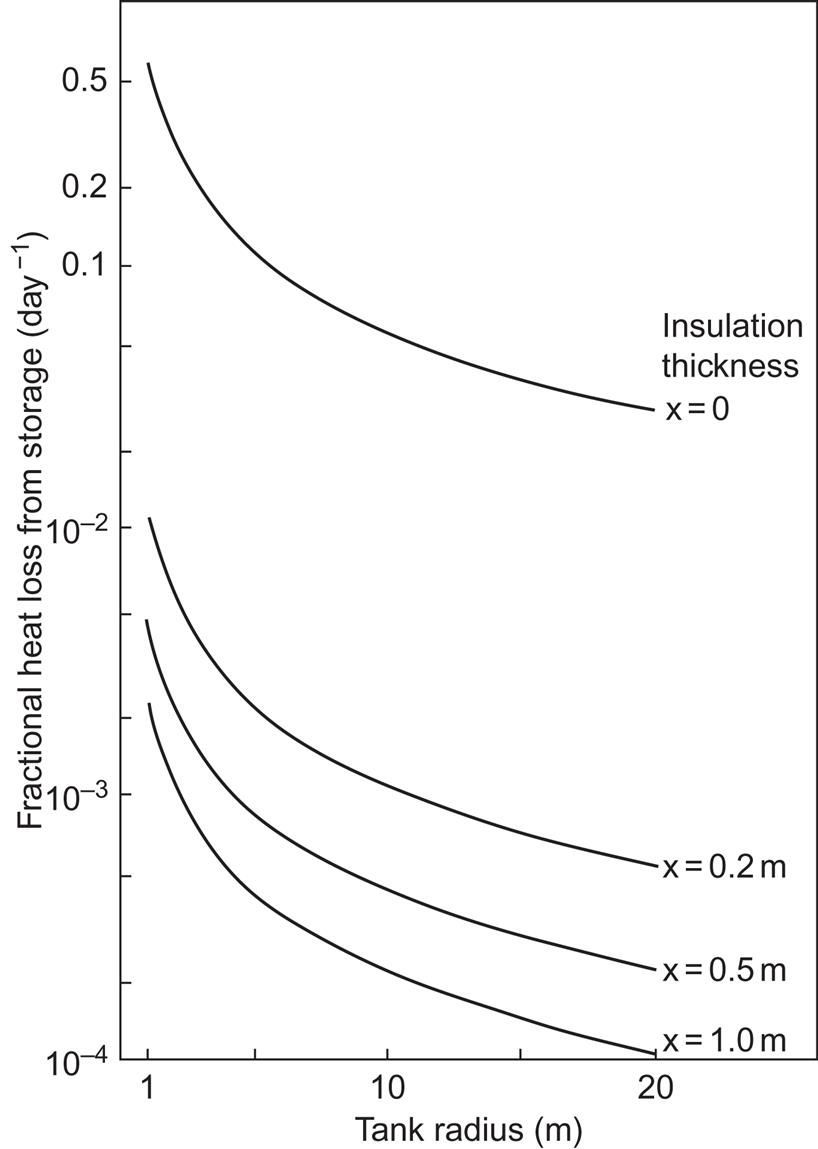
where R and L are radius and height of the cylinder, Ts is the average temperature of the water in the store, and Ta is the outside ambient air temperature. The fraction of the stored heat energy lost per unit time is
(5.6)
that is, the loss is independent of the temperatures and inversely proportional to a linear system dimension (cP is heat capacity and ρ is density).
Figure 5.5 shows, for L=3 R, the ratio of heat loss rate Ploss and stored energy Esens, according to (5.6), as a function of R and for different values of insulation thickness. This ratio is independent of the temperature difference, owing to the linear assumption for the heat loss rate. If the storage times required imply maximal fractional losses of 10%–20%, un-insulated tanks in the size range 5 m ≤ R ≤ 20 m are adequate for a few days of storage. If storage times around a month are required, some insulation must be added to tanks in the size range under consideration. If seasonal storage is needed, the smallest tank sizes will not work, even with a meter of mineral or glass wool wrapping. Community-size tanks, however, may serve for seasonal storage, with a moderate amount of insulation (0.2 m in the specific example).
A hot water tank with R=11.5 m and L=32 m has been used since 1978 by a utility company in Odense, Denmark, in connection with combined production of electricity and heat for district heating (Jensen, 1981). The hot water store is capable of providing all necessary heating during winter electricity peak hours, during which the utility company wants maximal electricity production. With a hot water store two or three times larger, the co-generating power units could be allowed to follow the electricity demand, which is small relative to the heat demand during winter nights.
A hot water store of similar magnitude, around 13 000 m3, may serve a solar-heated community system for 50–100 one-family houses, connected to the common storage facility by district heating lines. The solar collectors may still be on individual rooftops, or they may be placed centrally, for example, in connection with the store. In the first case, more piping and labor are required for installation, but in the second case, land area normally has to be dedicated to the collectors. Performance is also different for the two systems, as long as the coverage by solar energy is substantially less than 100% and the auxiliary heat source feeds into the district heating lines. The reason is that when the storage temperature is below the minimum required, the central solar collector will perform at high efficiency (Fig. 5.3), whereas individual solar collectors will receive input temperatures already raised by the ancillary heat source and thus will not perform as well. Alternatively, auxiliary heat could be added by individual installations on the load side of the system, but, unless the auxiliary heat is electrically generated, generating auxiliary heat is inconvenient if the houses do not already have a fuel-based heating system.
Most cost estimates argue against placing storage containers in air. If the container is buried underground (possibly with its top facing the atmosphere), the heat escaping the container will not be rapidly mixed into the surrounding soil or rock. Instead, the region closest to the container will reach a higher temperature, and a temperature gradient through the soil or rock will slowly build up. An exception is soil with ground water infiltration, because the moving water helps to mix the heat from the container into the surroundings. However, if a site can be found with no ground water (or at least no ground water in motion), then the heat loss from the store will be greatly reduced, and the surrounding soil or rock can be said to function as an extension of the storage volume.
As an example, consider a spherical water tank embedded in homogeneous soil. The tank radius is denoted R, the water temperature is Ts, and the soil temperature far away from the water tank is T0. If the transport of heat can be described by a diffusion equation, then the temperature distribution as function of distance from the center of the storage container may be written (Shelton, 1975)
(5.7)
where the distance r from the center must be larger than the tank radius R in order for the expression to be valid. The corresponding heat loss is
(5.8)
where λ is the heat conductivity of the soil and (5.8) gives the heat flux out of any sphere around the store of radius r ≥ R. The flux is independent of r. The loss relative to the heat stored in the tank itself is
(5.9)
The relative loss from the earth-buried store declines more rapidly with increasing storage size than the loss from a water store in air or other well-mixed surroundings [cf. (5.6)]. The fractional loss goes as R−2 rather than as R−1.
Practical considerations in building an underground or partly underground water store suggest an upside-down obelisk shape and a depth around 10 m for a 20 000-m2 storage volume. The obelisk is characterized by tilting sides, with a slope as steep as feasible for the soil type encountered. The top of the obelisk (the largest area end) would be at ground level or slightly above it, and the sides and bottom would be lined with plastic foil not penetrable by water. Insulation between lining and ground can be made with mineral wool foundation elements or similar materials. As a top cover, a sailcloth held in a bubble shape by slight overpressure is believed to be the least expensive solution. Top insulation of the water in the store can be floating foam material. If the sailcloth bubble is impermeable to light, algae growth in the water can be avoided (Danish Department of Energy, 1979).
Two community-size seasonal hot water stores placed underground have been operating in Sweden for a long time. They are both shaped as cut cones. One is in Studsvik. Its volume is 610 m3, and 120 m2 of concentrating solar collectors float on the top insulation, which can be turned to face the sun. Heat is provided for an office building with a floor area of 500 m2. The other system is in the Lambohov district of Linköping. It serves 55 semidetached one-family houses having a total of 2600 m2 flat-plate solar collectors on their roofs. The storage is 10 000 m3 and situated in solid rock (excavated by blasting). Both installations have operated since 1979, and they furnish a large part of the heat loads of the respective buildings. Figure 5.6 gives the temperature changes by season for the Studsvik project (Andreen and Schedin, 1980; Margen, 1980; Roseen, 1978).

Another possibility is to use existing ponds or lake sections for hot water storage. Top insulation would normally be required, and, in the case of lakes used only in part, an insulating curtain should separate the hot and cold water.
Keeping the time derivative in (3.35), a numerical integration will add information about the time required for reaching the steady-state situation. According to calculations like Shelton’s (1975), this may be about 1 year for typical large heat stores.
The assumption of a constant temperature throughout the storage tank may not be valid, particularly not for large tanks, owing to natural stratification that leaves the colder water at the bottom and the warmer water at the top. Artificial mixing by mechanical stirring is, of course, possible, but for many applications, temperature stratification is preferable. It could be used to advantage, for example, with storage tanks in a solar heating system (see Fig. 4.84), by feeding the collector with the colder water from the lower part of the storage and thus improving the efficiency (4.132) of the solar collector.
An alternative would be to divide the tank into physically separated subunits (cf., for example, Duffie and Beckman, 1974), but this requires a more elaborate control system to introduce and remove heat from the different units in an optimized way, and, if the storage has to be insulated, the subunits should at least be placed with common boundaries (tolerating some heat transfer among the units) in order to keep the total insulation requirement down.
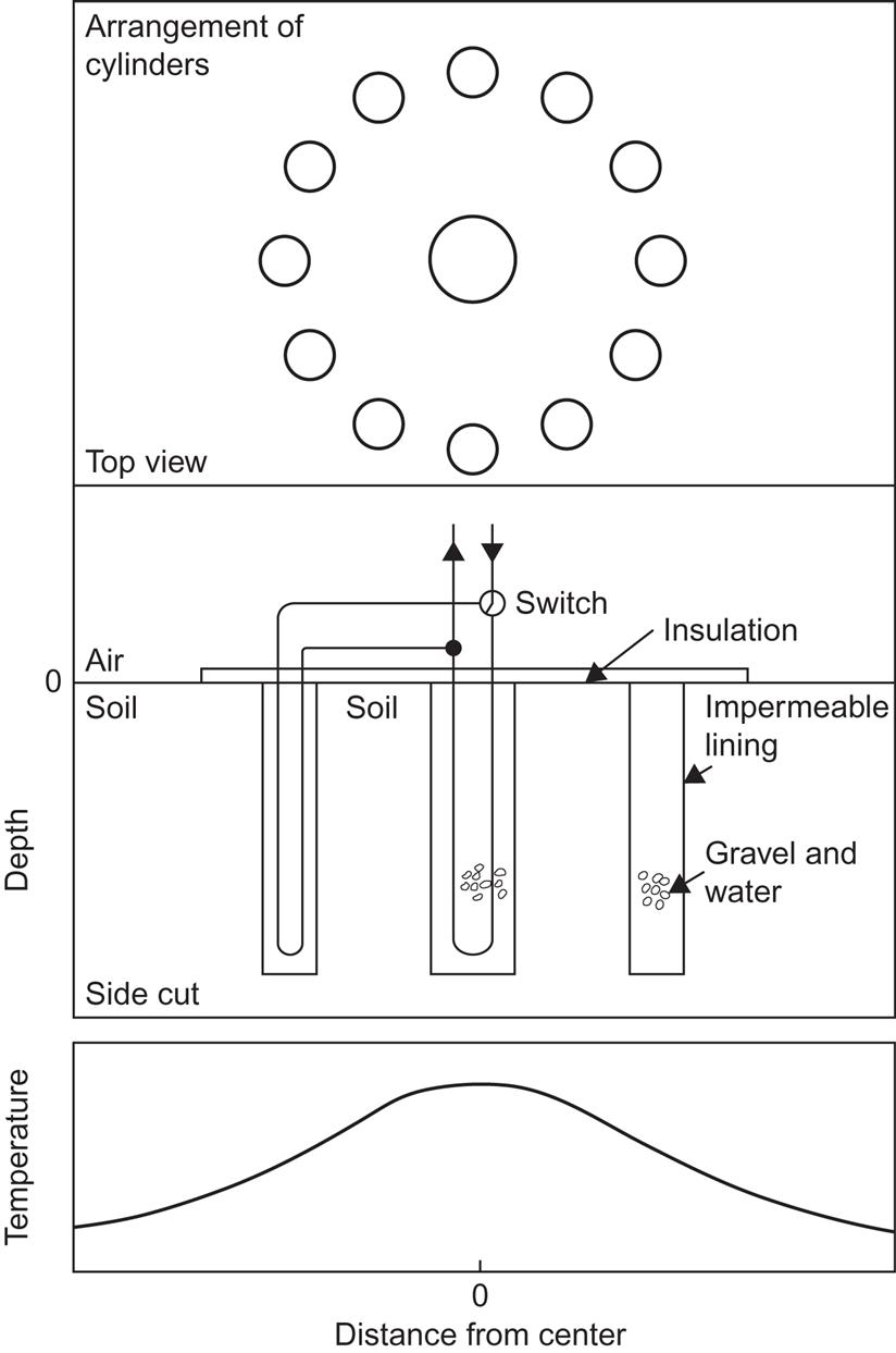
Multi-unit storage systems may be most appropriate for uninsulated storage in the ground, owing to the participation of the soil between the storage units. Figure 5.7 shows a possible arrangement (Brüel et al., 1976) based on cylindrical heat exchangers placed in one or more circles around a central heat exchanger cylinder in the soil. If no active aquifers traverse the soil region, a steady-state temperature distribution with a high central temperature can be built up. For example, with a flat-plate solar collector, the fluid going to the collector circuit could come from a low-temperature source and the fluid returning from the solar collector could be delivered to successive heat exchangers of diminishing temperatures in order to maximize the collector efficiency as well as the amount of heat transferred to storage. Dynamic simulations of storage systems of this type, using a solution of (3.33) with definite boundary conditions and source terms, have been performed by Zlatev and Thomsen (1976).
Other materials, such as gravel, rock, or soil, have been considered for use in heating systems at temperatures similar to those relevant for water. Despite volume penalties of a factor of 2–3 (depending on void volume), these materials may be more convenient than water for some applications. The main problem is to establish a suitable surface for the transfer of heat to and from the storage. For this reason, gravel and rock stores have been mostly used with air as a transfer fluid, because large volumes of air can be blown through the porous material.
For applications in other temperature ranges, other materials may be preferred. Iron (e.g., scrap material) is suitable for temperatures extending to several hundred degrees Celsius. In addition, for rock-based materials, the temperatures would not be limited to the boiling point of water.
5.2.3.1 Solar ponds and aquifer storage
A solar pond is a natural or artificial hot water storage system much like the ones described above, but with the top water surface exposed to solar radiation and operating like a solar collector. In order to achieve both collection and storage in the same medium, layers from top to bottom have to be inversely stratified, that is, stratified with the hottest zone at the bottom and the coldest one at the top. This implies that thermal lift must be opposed, either by physical means, such as placing horizontal plastic barriers to separate the layers, or by creating a density gradient in the pond, which provides gravitational forces to overcome the buoyancy forces. This can be done by adding certain salts to the pond, taking advantage of the higher density of the more salty water (Rabl and Nielsen, 1975).
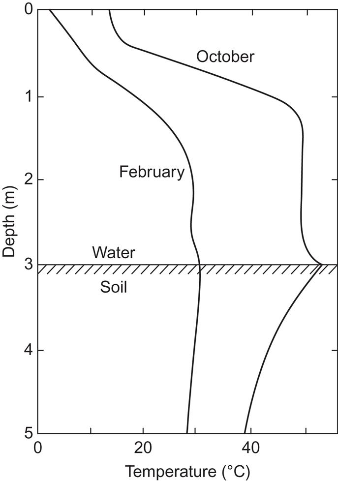
An example of a solar pond of obelisk shape is the 5200 m3 pond in Miamisburg, Ohio. Its depth is 3 m, and the upper half is a salt-gradient layer of NaCl, varying from 0% at the top to 18.5% at a depth of 1.5 m. The gradient opposes upward heat transport and thus functions as a top insulation without impeding the penetration of solar radiation. The bottom layer has a fixed salt concentration (18.5%) and contains heat exchangers for withdrawing energy. In this layer, convection may take place without problems. Most absorption of solar radiation takes place at the pond’s bottom surface (which is why the pond should be shallow), and the heat is subsequently released to the convective layer. At the top, however, some absorption of infrared solar radiation may destroy the gradient of temperature.
Figure 5.8 shows temperature gradients for the Miamisburg pond during its initial loading period (no load connected). After the start of operation in late August, the first temperature maximum occurred in October, and the subsequent minimum occurred in February. The two situations are shown in Fig. 5.8. The temperature in the ground just below the pond was also measured. In October, top-layer disturbance can be seen, but in February, it is absent, due to ice covering the top of the pond.
Numerical treatment of seasonal storage in large top-insulated or solar ponds may be done by time simulation, or by a simple approximation, in which solar radiation and pond temperature are taken as sine functions of time, with only the amplitude and phase as parameters to be determined. This is a fairly good approximation because of the slow response of a large seasonal store, which tends to be insensitive to rapid fluctuations in radiation or air temperature. However, when heat is extracted from the store, it must be ensured that disturbance of the pond’s temperature gradient will not occur, say, on a particularly cold winter day, where the heat extraction is large. Still, heat extraction can, in many cases, also be modeled by sine functions, and if the gradient structure of the pond remains stable, such a calculation gives largely realistic results.
In Israel, solar ponds are operated for electricity generation by use of Rankine cycle engines with organic working fluids that respond to the small temperature difference available. A correspondingly low thermodynamic efficiency must be accepted (Winsberg, 1981).
Truly underground storage of heat may also take place in geological formations capable of accepting and storing water, such as rock caverns and aquifers. In the aquifer case, it is important that water transport be modest, that is, that hot water injected at a given location stay approximately there and exchange heat with the surroundings only by conduction and diffusion processes. In such cases, it is estimated that high cycle efficiencies (85% at a temperature of the hot water some 200°C above the undisturbed aquifer temperature—the water being under high pressure) can be attained after breaking the system in, that is, after having established stable temperature gradients in the surroundings of the main storage region (Tsang et al., 1979).
5.2.4 Medium-and high-temperature storage
In industrial processes, temperature regimes are often defined as medium in the interval from 100°C to 500°C and as high above 500°C. These definitions may also be used in relation to thermal storage of energy, but it also may be useful to single out the lower-medium temperature range from 100°C to about 300°C, as the discussion below indicates.
Materials suitable for heat storage should have a large heat capacity, they must be stable in the temperature interval of interest, and it should be convenient to add heat to, or withdraw heat from, them.
The last of these requirements can be fulfilled in different ways. Either the material itself should possess good heat conductivity, as metals do, for example, or it should be easy to establish heat transfer surfaces between the material and some other suitable medium. If the transfer medium is a liquid or a gas, it could be passed along the transfer surface at a velocity sufficient for the desired heat transfer, even if the conductivities of the transfer fluid and the receiving or delivering material are small. If the storage material is arranged in a finite geometry, such that insufficient transfer is obtained by a single pass, then the transfer fluid may be passed along the surface several times. This is particularly relevant for transfer media like air, which has very low heat conductivity. When air is used as a transfer fluid, it is important that the effective transfer surface be large, and this may be achieved for granular storage materials like pebble or rock beds, where the nodule size and packing arrangement can be such that air can be forced through and reach most of the internal surfaces with as small an expenditure of compression energy as possible.
These considerations lie behind the approaches to sensible heat storage that are exemplified by the range of potential storage materials listed in Table 5.1. Some are solid metals, where transfer has to be by conduction through the material. Others are solids that may exist in granular form, for heat transfer by air or another gas blown through the packed material. They exhibit more modest heat conductivity. The third group comprises liquids, which may serve as both heat storage materials and transfer fluids. The dominating path of heat transfer may be conduction, advection (moving the entire fluid), or convection (turbulent transport). For highly conducting materials, such as liquid sodium, little transfer surface is required, but for the other materials listed, substantial heat exchanger surfaces may be necessary.
Table 5.1
Heat capacities of various materials (Kaye and Laby, 1959; Kreider, 1979; Meinel and Meinel, 1976). All quantities have some temperature dependence. Standard atmospheric pressure has been assumed, that is, all heat capacities are cP
| Material | Temperature Interval (°C) | Mass Spec. Heat (kJ kg−1 °C−1) | Volume Spec. Heat (MJ m−3 °C−1) | Heat Conductivity (W m−1 °C−1) |
| Solids | ||||
| Sodium chloride | <800 | 0.92 | 2.0 | 9a,b |
| Iron (cast) | <1500 | 0.46 | 3.6 | 70b−34c |
| Rock (granite) | <1700 | 0.79 | 2.2 | 2.7b |
| Bricks | 0.84 | 1.4 | 0.6 | |
| Earth (dry) | 0.79 | 1.0 | 1.0 | |
| Liquids | ||||
| Water | 0−100 | 4.2 | 4.2 | 0.6 |
| Oil (“thermal”) | −50 to 330 | 2.4 | 1.9 | 0.1 |
| Sodium | 98 to 880 | 1.3 | 1.3 | 85b−60c |
| Diethylene glycol | −10 to 240 | 2.8 | 2.9 | |
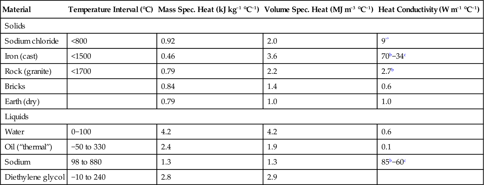
aLess for granulates with air-filled voids.
bAt 1000°C.
cAt 700°C.
Solid metals, such as cast iron, have been used for high-temperature storage in industry. Heat delivery and extraction may be accomplished by passing a fluid through channels drilled into the metal. For the medium- to high-temperature interval, the properties of liquid sodium (cf. Table 5.1) make it a widely used material for heat storage and transport, despite serious safety problems (sodium reacts explosively with water). It is used in nuclear breeder reactors and in concentrating solar collector systems, for storage at temperatures between 275°C and 530°C in connection with generation of steam for industrial processes or electricity generation. The physics of heat transfer to and from metal blocks and of fluid behavior in pipes is a standard subject covered in several textbooks (see, for example, Grimson, 1971).
Fixed beds of rock or granulate can be used for energy storage at both low and high temperatures. Normally, air is blown through the bed to transfer heat to and from the store. The pressure drop ΔP across a rock bed of length L, such as the one illustrated in Fig. 5.9, where air is blown through the entire cross-sectional area A, may be estimated as (Handley and Heggs, 1968)
(5.10)
where ρa and va are density and velocity of the air passing through the bed in a steady-state situation, ds is the equivalent spherical diameter of the rock particles, and m, their mixing ratio, is one minus the air fraction in the volume L×A. Re is the Reynolds number describing the ratio between “inertial” and “viscous” forces on the air passing between the rock particles. Re may be estimated as ρavada/μ, where μ is the dynamic viscosity of air. If the rock particles are not spherical, the equivalent diameter may be taken as
where n is the number of particles in the entire bed volume. The estimate (5.10) assumes the bed to be uniform and the situation stationary. The total surface area of the particles in the bed is given by

Optimal storage requires that the temperature gradient between the particle surfaces and their interior be small and that the pressure drop (5.10) also be small, leading to optimal particle diameters of a few centimeters and a void fraction of about 0.5 (implying that ms is also about 0.5).
Organic materials, such as diethylene glycol or special oil products (Table 5.1), are suitable for heat storage between 200°C and 300°C and have been used in concentrating solar collector test facilities (Grasse, 1981). Above 300°C, the oil decomposes.
Despite low-volume heat capacities, gaseous heat storage materials could also be considered. For example, steam (water vapor) is often stored under pressure, in cases where it is the form of heat energy to be used later (in industrial processes, power plants, etc.).
5.3 Latent heat and chemical transformation storage
The energy associated with a phase change for a material can be used to store energy. The phase change may be melting or evaporating, or it may be associated with a structural change, e.g., in lattice form, content of crystal-bound water, etc. When heat is added to or removed from a material, a number of changes may take place successively or in some cases simultaneously, involving phase changes as well as energy storage in thermal motion of molecules, i.e., both latent and sensible heat. The total energy change, which can serve as energy storage, is given by the change in enthalpy.
Solid–solid phase transitions are observed in one-component, binary, and ternary systems, as well as in single elements. An example of the latter is solid sulfur, which occurs in two different crystalline forms, a low-temperature orthorhombic form and a high-temperature monoclinic form (cf. Moore, 1972). However, the elementary sulfur system has been studied merely out of academic interest, in contrast to the practical interest in the one-component systems listed in Table 5.2. Of these systems, which have been studied for practical energy storage, Li2SO4 exhibits both the highest transition temperature Tt and the highest latent heat for the solid–solid phase change ΔHss. Pure Li2SO4 undergoes a transition from a monoclinic to a face-centered cubic structure with a latent heat of 214 KJ kg−1 at 578°C. This is much higher than the heat of melting (−67 KJ kg−1 at 860°C). Another one-component material listed in Table 5.2 is Na2SO4, which has two transitions at 201°C and 247°C, with the total latent heat of both transitions being ~80 KJ kg−1.
Table 5.2
Solid–solid transition enthalpies ΔHss (Fittipaldi, 1981)
| Material | Transition Temperature Tt (°C) | Latent Heat ΔHss (kJ kg−1) |
| V2O2 | 72 | 50 |
| FeS | 138 | 50 |
| KHF2 | 196 | 135 |
| Na2SO4 | 210, 247 | 80 |
| Li2SO4 | 578 | 214 |
Mixtures of Li2SO4 with Na2SO4 and K2SO4 with ZnSO have also been studied, as well as some ternary mixtures containing these and other sulfates (in a Swedish investigation, Sjoblom, 1981). Two binary systems (Li2SO4−Na2SO4, 50 mol% each, Tt=518°C; and 60% Li2SO4−40% ZnSO4, Tt=459°C) have high values of latent heat, ~190 KJ kg−1, but they exhibit a strong tendency for deformation during thermal cycling. A number of ternary salt mixtures based on the most successful binary compositions have been studied experimentally, but knowledge of phase diagrams, structures, and re-crystallization processes that lead to deformation in these systems is still lacking.
5.3.1 Salt hydrates
The possibility of energy storage by use of incongruently melting salt hydrates has been intensely investigated, starting with the work of Telkes (1952, 1976). Molten salt consists of a saturated solution as well as some un-dissolved anhydrous salt because of its insufficient solubility at the melting temperature, considering the amount of released crystal water available. Sedimentation will develop, and a solid crust may form at the interface between layers. To control this, stirring is applied, for example, by keeping the material in rotating cylinders (Herrick, 1982), and additives are administered in order to control agglomeration and crystal size (Marks, 1983).
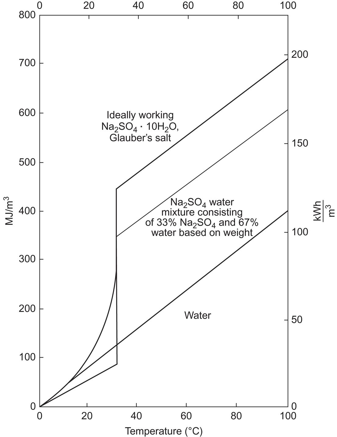
An alternative is to add extra water to prevent phase separation. This has led to a number of stable heat-of-fusion storage systems (Biswas, 1977; Furbo, 1982). Some melting points and latent heats of salt hydrates are listed in Table 5.3. Here we use as an example Glauber salt (Na2SO4 · 10H2O), the storage capacity of which is illustrated in Fig. 5.10, both for the pure hydrate and for a 33% water mixture used in actual experiments. Long-term verification of this and other systems in connection with solar collector installations have been carried out by the European Economic Community. For hot water systems, the advantage over sensible heat water stores is minimal, but this may change when space heating is included, because of the seasonal storage need (Furbo, 1982).
Table 5.3
Characteristics of salt hydrates
| Hydrate | Incongruent Melting Point, Tm (°C) | Specific Latent Heat ΔH (MJ m−3) |
| CaCl2·6H2O | 29 | 281 |
| Na2SO4·10H2O | 32 | 342 |
| Na2CO3·10H2O | 33 | 360 |
| Na2HPO4·12H2O | 35 | 205 |
| Na2HPO4·7H2O | 48 | 302 |
| Na2S2O3·5H2O | 48 | 346 |
| Ba(OH)2·8H2O | 78 | 655 |
Salt hydrates release water when heated and release heat when they are formed. The temperatures at which the reaction occurs vary for different compounds, ranging from 30°C to 80°C, which makes possible a range of storage systems for a variety of water-based heating systems, such as solar, central, and district heating. Table 5.3 shows the temperatures Tm of incongruent melting and the associated quasi-latent heat Q (or ΔH) for some hydrates that have been studied extensively in heat storage system operation. The practical use of salt hydrates faces physicochemical and thermal problems, such as supercooling, incongruent melting, and heat transfer difficulties imposed by locally low heat conductivities (cf., for example, Achard et al., 1981).
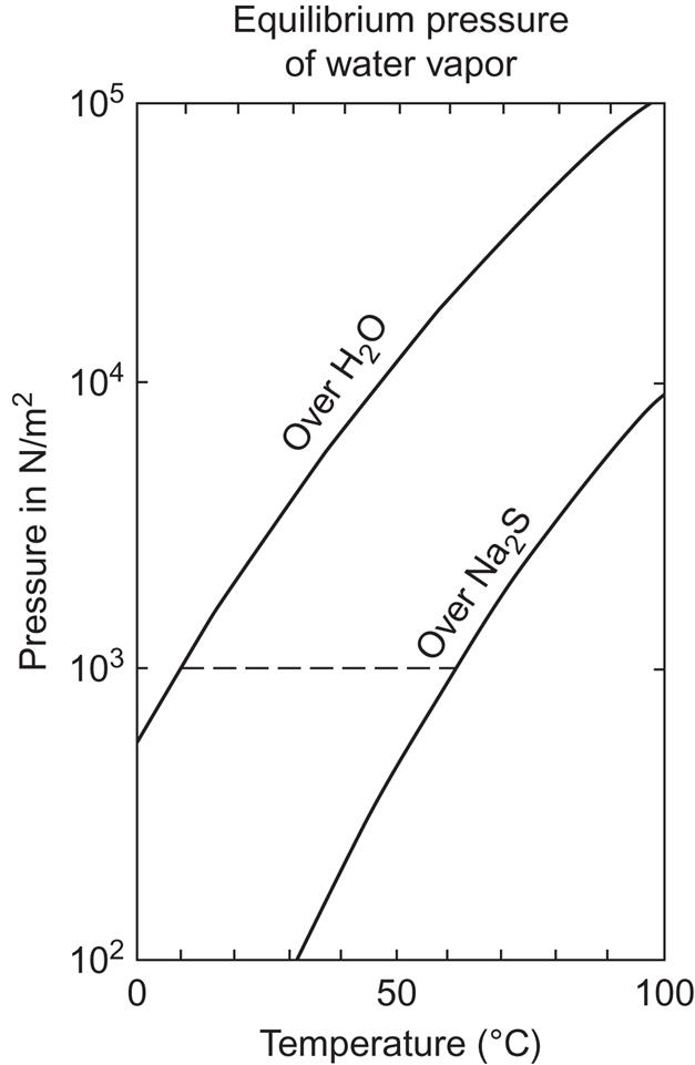
Generally, storage in a chemical system with two separated components, of which one draws low-temperature heat from the environment and the other absorbs or delivers heat at fairly low (30°C−100°C) or medium (100°C−200°C) temperature, is referred to as a chemical heat pump (McBride, 1981). Simply stated, the chemical heat pump principle consists in keeping a substance in one of two containers, although it would prefer to be in the other one. In a classical example, the substances are water vapor and sulfuric acid. Because the pressure over sulfuric acid is much lower than over liquid water (see Fig. 5.11), water vapor will move from the water surface to the H2SO4 surface and become absorbed there, with a heat gain deriving in part from the mixing process and in part from the heat of evaporation. The temperature of the mixture is then above what is needed at the water source. Heat is stored when the temperature of the sulfuric acid/water container is made still higher, so that the equilibrium pressure of vapor above the acid surface at this temperature becomes higher than that above the water surface at its temperature. The pressure gradient will therefore move water vapor back to the water surface for condensation.

A similar system, but with the water being attached as crystal water in a salt (i.e., salt hydration), is the sodium sulfide (Na2S)/water system earlier developed in Sweden (System Tepidus; Bakken, 1981). Figure 5.12 shows this chemical heat pump, which is charged by the reaction
(5.11)

The heat for the evaporation is taken from a reservoir of about 5°C, that is, a pipe extending through the soil at a depth of a few meters (as in commercial electric heat pumps with the evaporator buried in the lawn), corresponding to roughly 10°C in the water container (B in Fig. 5.12) owing to heat-exchanger losses. The water vapor flows to the Na2S container (A in Fig. 5.12) through a connecting pipe that has been evacuated of all gases other than water vapor and where the water vapor pressure is of the order of 1% of atmospheric pressure. During charging, the temperature in the sodium sulfide rises to 65 °C–70°C, owing to the heat formed in the process (5.11). When the temperatures in containers A and B and the equilibrium pressures of the water vapor are such that they correspond to each other by a horizontal line in the pressure–temperature diagram shown in Fig. 5.13, flow stops and container A has been charged.
To release the energy, a load area of temperature lower than that of container A is connected to it and heat is transferred through a heat exchanger. Lowering the temperature in A causes a pressure gradient to form in the connecting pipe, and new energy is drawn from B to A. In order to prevent the heat reservoir (the soil) from cooling significantly, new heat must be added to compensate for the heat withdrawn. This takes place continuously by transfer processes in the soil (solar radiation absorbed at the soil surface is conducted to the subsurface location of the evaporator pipes). However, in the long term, a lower temperature would develop in the soil environment if no active makeup heat were supplied. This is done by leading surplus heat from a solar collector to the sodium sulfide container when the solar heat is not directly required in the load area. When the temperature of container A is raised in this way, the pressure gradient above the salt will drive water vapor to container B, thereby removing some of the crystallization water from the salt.
The two actual installations of this type of chemical heat pump are a one-family dwelling with a storage capacity of 7000 kWh (started in 1979) and an industrial building (Swedish Telecommunications Administration) with 30 000 kWh of storage, started in 1980. Future applications may comprise transportable heat stores, since container A may be detached (after closing the valve indicated in Fig. 5.12) and carried to another site. Once the container is detached, the sensible heat is lost, as the container cools from its 60°C to ambient temperatures, but this amounts to only 3%−4% of the energy stored in the Na2S·5H2O (Bakken, 1981).
It should be mentioned that a similar loss occurs during use of the storage unit in connection with a solar heating system. This is because of the intermittent call upon the store. Every time it is needed, its temperature increases to 60°C (i.e., every time the valve is opened), using energy to supply the sensible heat, and every time the need starts to decrease, there is a heat loss associated either with making up for the heat transfer to the surroundings (depending on the insulation of the container) to keep the container temperature at 60°C or, if the valve has been closed, with the heat required to reheat the container to its working temperature. These losses could be minimized by using a modular system, where only one module at a time is kept at operating temperature, ready to supply heat if the solar collector is not providing enough. The other modules would then be at ambient temperatures except when they are called upon to recharge or to replace the unit at standby.
The prototype systems are not cost effective, but the estimated system cost in regular production is 4−5 euro per kWh of heat supplied to a 15 m3 storage system for a detached house, with half the cost incurred by the solar collector system and the other half incurred by the store. For transport, container sizes equivalent to 4500 kWh of 60°C heat are envisaged. However, the charge-rate capacity of roughly 1 W kg−1 may be insufficient for most applications.
Although the application of the chemical heat pump considered above is for heating, the concept is equally useful for cooling. Here the load would simply be connected to the cold container. Several projects are underway to study various chemical reactions of the gas/liquid or gas/solid type based on pressure differences, either for cooling alone or for both heating and cooling. The materials are chosen on the basis of their temperature requirements and long-term stability while allowing many storage cycles. For example, NaI–NH3 systems have been considered for air conditioning purposes (Fujiwara et al., 1981). A number of ammoniated salts that react on heat exchange could also be considered.
5.3.2 Chemical reactions
The use of high-temperature chemical heat reactions in thermal storage systems is fairly new and to some extent related to attempts to utilize high-temperature waste heat and to improve the performance of steam power plants (cf. Golibersuch et al., 1976). The chemical reactions that are used to store the heat allow, in addition, upgrading of heat from a lower temperature level to a higher temperature level, a property that is not associated with phase transition or heat capacity methods.
Conventional combustion of fuel is a chemical reaction in which the fuel is combined with an oxidant to form reaction products and surplus heat. This type of chemical reaction is normally irreversible, and there is no easy way that the reverse reaction can be used to store thermal energy. The process of burning fuel is a chemical reaction whereby energy in one form (chemical energy) is transformed into another form (heat) accompanied by an increase in entropy. In order to use a chemical reaction for storage of heat, it would, for example, in the case of hydrocarbon, require a reverse process whereby the fuel (hydrocarbon) could be obtained by adding heat to the reaction products carbon dioxide and water. Therefore, use of chemical heat reactions for thermal energy storage requires suitable reversible reactions.
The change in bond energy for a reversible chemical reaction may be used to store heat, but although a great variety of reversible reactions are known, only a few have so far been identified as being technically and economically acceptable candidates. The technical constraints include temperature, pressure, energy densities, power densities, and thermal efficiency. In general, a chemical heat reaction is a process whereby a chemical compound is dissociated by heat absorption, and later, when the reaction products are recombined, the absorbed heat is again released. Reversible chemical heat reactions can be divided into two groups: thermal dissociation reactions and catalytic reactions. The thermal dissociation reaction may be described as
(5.12)
indicating that dissociation takes place by addition of heat ΔH to AB at temperature T1 and pressure p1, whereas heat is released (−ΔH) in the reverse reaction at temperature T2 and pressure p2. The reciprocal reaction (from right to left) occurs spontaneously if the equilibrium is disturbed, that is, if T2<T1 and p2>p1. To avoid uncontrolled reverse reaction, the reaction products must therefore be separated and stored in different containers. This separation of the reaction products is not necessary in catalytic reaction systems, where both reactions (left to right and right to left) require a catalyst in order to obtain acceptable high reaction velocities. If the catalyst is removed, neither of the reactions will take place even when considerable changes in temperature and pressure occur. This fact leads to an important advantage, namely, that the intrinsic storage time is, in practice, very large and, in principle, infinite. Another advantage of closed-loop heat storage systems employing chemical reactions is that the compounds involved are not consumed, and because of the high energy densities (in the order of magnitude: 1 MWh m−3, compared to that of the sensible heat of water at ΔT=50 K, which is 0.06 MWh m−3), a variety of chemical compounds are economically acceptable.
The interest in high-temperature chemical reactions is derived from the work of German investigators on the methane reaction
(5.13)
(Q being heat added), which was studied in relation to long-distance transmission of high-temperature heat from nuclear gas reactors (cf. Schulten et al., 1974). The transmission system called EVA-ADAM, an abbreviation of the German Einzelrorhrversuchsanlage und Anlage zur dreistufigen adiabatischen Methanisierung, is being further developed at the nuclear research center at Jülich, West Germany. It consists of steam reforming at the nuclear reactor site, transport over long distances of the reformed gas (CO + 3H2), and methanation at the consumer site, where heat for electricity and district heating is provided (cf., for example, Harth et al., 1981).
The reaction in (5.13) is a suitable candidate for energy storage that can be accomplished as follows: heat is absorbed in the endothermic reformer, where the previously stored low-enthalpy reactants (methane and water) are converted into high-enthalpy products (carbon monoxide and hydrogen). After heat exchange with the incoming reactants, the products are then stored in a separate vessel at ambient temperature conditions, and although the reverse reaction is thermodynamically favored, it will not occur at these low temperatures and in the absence of a catalyst. When heat is needed, the products are recovered from storage and the reverse, exothermic reaction (methanation) is run (cf. Golibersuch et al., 1976). Enthalpies and temperature ranges for some high-temperature closed-loop C-H-O systems, including reaction (5.13), are given in Table 5.4. The performance of the cyclohexane to benzene and hydrogen system (listed fourth in Table 5.4) has been studied in detail by Italian workers, and an assessment of a storage plant design has been made (cf. Cacciola et al., 1981). The complete storage plant consists of hydrogenation and dehydrogenation multistage adiabatic reactors, storage tanks, separators, heat exchangers, and multistage compressors. Thermodynamic requirements are ensured by independent closed-loop systems circulating nitrogen in the dehydrogenation unit and hydrogen in the hydrogenation unit.
Table 5.4
High-temperature closed-loop chemical C-H-O reactions. (Hanneman et al., 1974; Harth et al., 1981)
| Closed-Loop System | Enthalpya ΔH0 (kJ mol−1) | Temperature Range (K) |
| CH4+H2O↔CO+3H2 | 206(250)b | 700−1200 |
| CH4+CO2↔2CO+2H2 | 247 | 700−1200 |
| CH4+2H2O↔CO2+4H2 | 165 | 500−700 |
| C6H12↔C6H6+3H2 | 207 | 500−750 |
| C7H14↔C7H8+3H2 | 213 | 450−700 |
| C10H18↔C10H8+5H2 | 314 | 450−700 |
aStandard enthalpy for complete reaction.
bIncluding heat of evaporation of water.
A number of ammoniated salts are known to dissociate and release ammonia at different temperatures, including some in the high-temperature range (see, for example, Yoneda et al., 1980). The advantages of solid–gas reactions in general are high heats of reaction and short reaction times. This implies, in principle, high energy and power densities. However, poor heat and mass transfer characteristics in many practical systems, together with problems of sagging and swelling of the solid materials, lead to reduced densities of the total storage system.
Metal hydride systems are primarily considered as stores of hydrogen, as is discussed later. However, they have also been contemplated for heat storage, and in any case, the heat-related process is integral in getting the hydrogen into and out of the hydride. The formation of a hydride MeHx (metal plus hydrogen) is usually a spontaneous exothermic reaction:
(5.14)
which can be reversed easily by applying the amount of heat Q,
(5.15)
Thus, a closed-loop system, where hydrogen is not consumed but is pumped between separate hydride units, may be used as a heat store. High-temperature hydrides, such as MgH2, Mg2NiH2, and TiH2, have, owing to their high formation enthalpies (e.g., for MgH2, ΔH≥80 kJ per mol of H2; for TiH2, ΔH>160 KJ per mol of H2), heat densities of up to 3 MJ kg−1 or 6 GJ m−3 in a temperature range extending from 100°C to 600°C (cf. Buchner, 1980).
5.4 High-quality energy storage
A number of storage systems may be particularly suitable for the storage of “high-quality” energy, such as mechanical energy or electric energy. If the energy to be stored is derived from a primary conversion delivering electricity, for example, then one needs an energy storage system that will allow the regeneration of electricity with high cycle efficiency, i.e., with a large fraction of the electricity input recovered in the form of electricity. Thermal stores, such as the options mentioned in the previous section, may not achieve this, even at T=800°C−1500°C (metals, etc.), because of the Carnot limit to the efficiency of electricity regeneration, as well as storage losses through insulation, etc. Thermal stores fed via a heat pump drawing from a suitable reference reservoir may reach tolerable cycle efficiencies more easily.
Table 5.5 gives an indication of the actual or estimated energy densities and cycle efficiencies of various storage systems. The theoretical maximum of energy density is, in some cases, considerably higher than the values quoted.
Table 5.5
Energy density by weight and volume for various storage forms, based on measured data or expectations for practical applications. For the storage forms aimed at storing and regenerating high-quality energy (electricity), cycle efficiencies are also indicated. Hydrogen gas density is quoted at ambient pressure and temperature. For compressed air energy storage, both electricity and heat inputs are included on equal terms in estimating the cycle efficiency. (Compiled with use of Jensen and Sørensen, 1984.)
| Storage Form | Energy Density | Cycle Efficiency | |
| kJ kg−1 | MJ m−3 | ||
| Conventional fuels | |||
| Crude oil | 42 000 | 37 000 | |
| Coal | 32 000 | 42 000 | |
| Dry wood | 12 500a | 10 000 | |
| Synthetic fuels | |||
| Hydrogen, gas | 120 000 | 10 | 0.4−0.6 |
| Hydrogen, liquid | 120 000 | 8700 | |
| Hydrogen, metal hydride | 2000−9000 | 5000−15 000 | |
| Methanol | 21 000 | 17 000 | |
| Ethanol | 28 000 | 22 000 | |
| Thermal–low quality | |||
| Water, 100°C→40°C | 250 | 250 | |
| Rocks, 100°C→40°C | 40−50 | 100−140 | |
| Iron, 100°C→40°C | ~30 | ~230 | |
| Thermal–high quality | |||
| Rocks, e.g., 400°C→200°C | ~160 | ~430 | |
| Iron, e.g., 400°C→200°C | ~100 | ~800 | |
| Inorganic salts, heat of fusion > 300°C | >300 | >300 | |
| Mechanical | |||
| Pumped hydro, 100 m head | 1 | 1 | 0.65−0.8 |
| Compressed air | ~15 | 0.4−0.5 | |
| Flywheels, steel | 30−120 | 240−950 | |
| Flywheels, advanced | >200 | > 100 | ~0.95 |
| Electrochemical | |||
| Lead–acid | 40−140 | 100−900 | 0.7−0.8 |
| Nickel–cadmium | ~350 | ~350 | varying |
| Lithium ion (other advanced batteries) | 700 (>400) | 1400 (>300) | 0.7 (>0.8) |
| Superconducting | ~100 | ~0.85 | |

aOven-dry wood may reach values up to 20 000 kJ kg−1.
For comparison, energy densities of thermal stores and a number of fuels are also given. Some of the fuels (methanol, wood, and hydrogen) may be produced by conversion based on renewable energy sources (without having to wait for fossilization processes to occur). The cycle efficiency is defined with the assumption that the initial energy form is electricity or another high-quality energy form, and the value quoted for hydrogen is based on electrolysis of water as the first step in the storage cycle. Methanol may also be reversibly transformed into hydrogen and carbon oxide to play the role of a closed storage cycle (Prengle and Sun, 1976). The most striking feature is the low-volume energy density of nearly all the reversible storage concepts considered, relative to that of solid or liquid fossil fuels.
The magnitudes of stores that might be associated with renewable energy use (such as indicated in Fig. 2.91) are discussed in more detail in section 6.3, with a summary in the tables of section 6.7, in connection with future energy scenario construction. For comparison, reservoirs of fossil fuels may be found in Table 4.2.
5.5 Pumped hydro storage
The total exploitable hydro potential is of the order of 1012 W on average over the year (section 3.3.2), and only the fraction of this associated with reservoirs can be considered relevant for energy storage. The river flows that have to be tapped as they come may be interesting as energy sources, but not as energy storage options.
Hydro reservoirs feeding into turbine power plants may be utilized for storage of electric energy generated by non-hydropower plants (e.g., wind or photovoltaic energy converters), provided that all the power plants are connected by a common grid, and provided that transmission capacity is sufficient to accommodate the extra burden of load-leveling storage operation of the system. The storage function in a system of this kind is primarily obtained by displacement of load. This means that the hydropower units are serving as backup for the non-hydro generators by providing power when non-hydropower production falls short of load. The small start-up time for hydro turbines (½−3 min) makes this mode of operation convenient. When there is surplus power generation from the non-hydro units, then the hydro generation is decreased, and non-hydro-produced power is transmitted to the load areas otherwise served by hydropower (Sørensen, 1981; Meibom et al., 1999). In this way, there is no need to pump water up into the hydro reservoirs, as long as the non-hydropower generation stays below the combined load of hydro and non-hydro load areas. To fulfill this condition, the relative sizes of the different types of generating units must be chosen carefully.
When the surplus energy to be stored exceeds the amounts that can be handled in the displacement mode described above, then upward pumping of water into the hydro reservoirs may be considered. It is accomplished by use of two-way turbines, so that the energy can be stored and recovered by the same installation. Alternatively, pumped storage may utilize natural or artificially constructed reservoirs not associated with any exploitable hydropower.
Figure 5.14 shows an example of the layout of a pumped storage facility. Installations where reservoirs are not part of a hydro flow system are typically intended for short-term storage. They may be used for load-leveling purposes, providing a few hours of peak load electric power per day, based on nighttime pumping. In terms of average load covered, the storage capacities of these installations are below 24 h. On the other hand, some of the natural reservoirs associated with hydro schemes have storage capacities corresponding to one or more years of average load (e.g., the Norwegian hydro system; cf. Sørensen, 1981; Meibom et al., 1999). Pumping schemes for such reservoirs could serve for long-term storage of energy.

If no natural elevated reservoirs are present, pumped storage schemes may be based on underground lower reservoirs and surface-level upper reservoirs. The upper reservoirs may be lakes or oceans. The lower ones should be excavated or should make use of natural cavities in the underground. If excavation is necessary, a network of horizontal mine shafts, such as the one illustrated in Fig. 5.15, may be employed in order to maintain structural stability against collapse (Blomquist et al., 1979; Hambraeus, 1975).
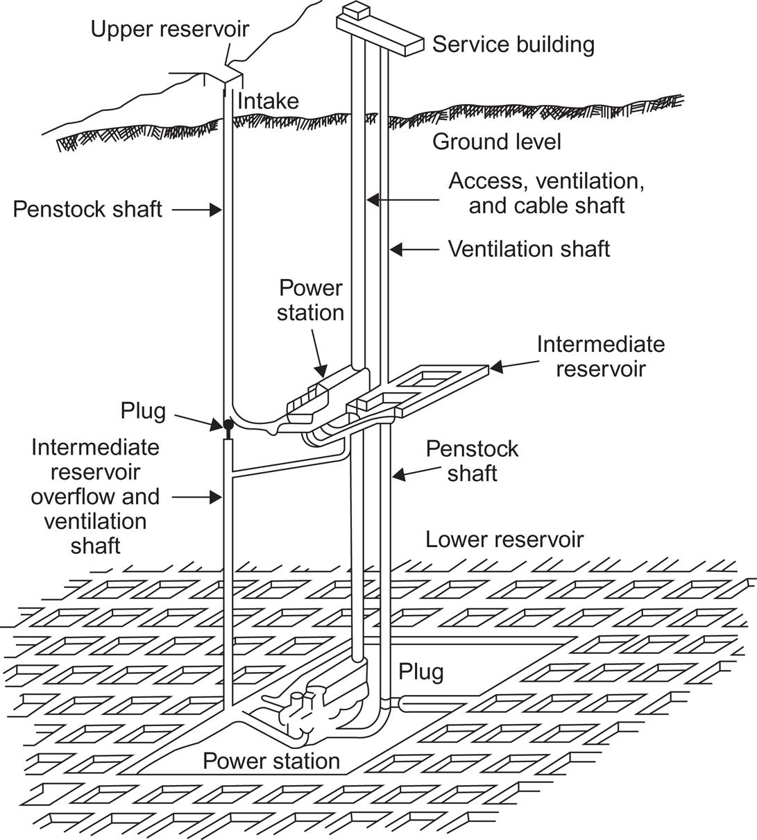
The choice of equipment is determined primarily by the size of head, that is, the vertical drop available between the upper and the lower reservoir. Figure 4.37 shows in a schematic form the three most common types of hydro turbines. The Kaplan turbine (called a Nagler turbine if the position of the rotor blades cannot be varied) is most suited for low heads, down to a few meters. Its rotor has the shape of a propeller, and the efficiency of converting gravitational energy into shaft power is high (over 0.9) for the design water velocity, but lower for other water speeds. The efficiency drop away from the design water velocity is rapid for the Nagler turbine, less so for the Kaplan version. These turbines are inefficient for upward pumping, although they can be made to accept water flow from either side (André, 1976). A displacement pump may be used in a “tandem arrangement” (i.e., separate turbine and pump). The electric generator is easily made reversible, so that it may serve either as generator or as motor.
For larger heads, the Francis and Pelton turbines may be used. Francis turbines have a set of fixed guiding blades leading the water onto the rotating blades (the runner) at optimum incident angle. It can be used with water heads up to about 600 m in the simple version illustrated in Fig. 4.37b, but multistage versions have been considered, guiding the water through a number of runners (five for an actual French installation; cf. Blomquist et al., 1979). In this way, heads above 1000 m can be accepted, and the arrangement may be completely reversible, with very modest losses. For either pumping or generating, the turbine efficiency at design water flow may be over 0.95, but for decreasing flow the efficiency drops. Typical overall efficiencies of the storage cycle (pumping water up by use of surplus electric power, regenerating electric power based on downward flow through turbines) are around 0.8 for existing one-stage Francis turbine installations. Shifting from pumping to generating takes about 1 min (Hambraeus, 1975). The total cycle efficiency of the multistage Francis turbines for heads of 1000–1500 m is about 0.7 (Blomquist et al., 1979).
If the head is larger than the limit for single-stage, reversible Francis turbines, an alternative to the multistage Francis turbines is offered by tandem units consisting of separate impulse turbines and pumps. The pump units for pumping upward over height differences exceeding 1000 m are usually multistage pumps (six stages for an actual installation in Italy), with efficiency over 0.9 being achieved. The impulse turbine part is of Pelton type (see Fig. 4.37a), consisting of a bucket-wheel being driven by the impulse of one or more water jets created by passing the water through nozzles. The power for this process is the pressure force created by the column of water, from the turbine placed at the lower reservoir level to the upper reservoir level. The pressure energy can be converted partially or fully into linear kinetic energy according to the requirements of the different turbine types,
Here the initial potential energy associated with the head Δz is transformed into a kinetic energy part associated with partial mass m′ moving with velocity u and a pressure energy part with the enthalpy H given by the pressure P over the density of water ρ, times the remaining mass m–m′. The conversion efficiency of Pelton turbines is about 0.9 over a wide range of power levels, and the tandem arrangement of separate turbine and pump (but with generator/motor, turbine, and pump all mounted on a common shaft) allows quick shifts between generating and pumping or vice versa.
The losses in conversion are associated in part with “leakage”, that is, with water that passes around the turbine without contributing to power, and in part with energy dissipation in the form of heat, for example, due to friction (cf. Angrist, 1976). Further losses are associated with evaporation of water, especially from solar-exposed upper reservoirs.
Excavation for underground storage limits the application to short-term storage (up to about 24 h of average load) because the cost scales approximately linearly with storage capacity. For large natural reservoirs, seasonal energy storage can be considered, since the cost has a large component determined by the maximum load requirement and therefore becomes fairly independent of storage capacity beyond a certain point, as long as the reservoir is available.
5.5.1 Flywheels
Mechanical energy may be stored in the form of rotational motion under conditions of low frictional losses. A flywheel is such a rotating structure, capable of receiving and delivering power through its shaft of rotation. Friction is diminished by use of high-performance bearings, and the entire rotating structure may be enclosed in a space with partial vacuum or filled with an inert gas.
The amount of energy stored in a body of mass distribution ρ (x) rotating about a fixed axis with angular velocity ω is
(5.16)
with the moment of inertia I given by
It appears from these expressions that high angular velocity and a majority of the mass situated at a large distance r from the axis of rotation would lead to high amounts of energy stored. The relevant question to ask, however, is how to obtain the highest energy density, given material of a certain strength.
The strength of materials is quantified as the tensile strength, defined as the highest stress not leading to a permanent deformation or breaking of the material. If the material is inhomogeneous, the breaking stresses, and hence the tensile strengths, are different in different directions. For fibrous materials, there are characteristic tensile strengths in the direction of the fibers and perpendicular to the direction of the fibers, the former in some cases being orders of magnitude larger than the latter.
The components in x-, y-, and z-directions of the force per unit volume, f, are related to the stress tensor τij by
(5.17)
and the tensile strength σI in a direction specified by i is
(5.18)
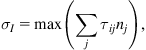 (5.18)
where n is a unit vector normal to the “cut” in the material (see Fig. 5.16) and the maximum sustainable stress in the direction i is to be found by varying the direction of n, that is, varying the angle of slicing. In other words, the angle of the cut is varied until the stress in the direction i is maximum, and the highest value of this maximum stress not leading to irreversible damage defines the tensile strength. If the material is isotropic, the tensile strength is independent of direction and may be denoted σ.
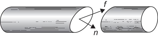
Consider now a flywheel like the one illustrated in Fig. 5.17, rotating with angular velocity ω about a fixed axis. The mass distribution is symmetric around the axis of rotation, that is, invariant with respect to rotations through any angle θ about the rotational axis. It is further assumed that the material is homogeneous, so that the mass distribution is fully determined by the mass density ρ and the variation of disk width b(r) as a function of radial distance r from the axis, for a shape symmetric about the midway plane normal to the axis of rotation.
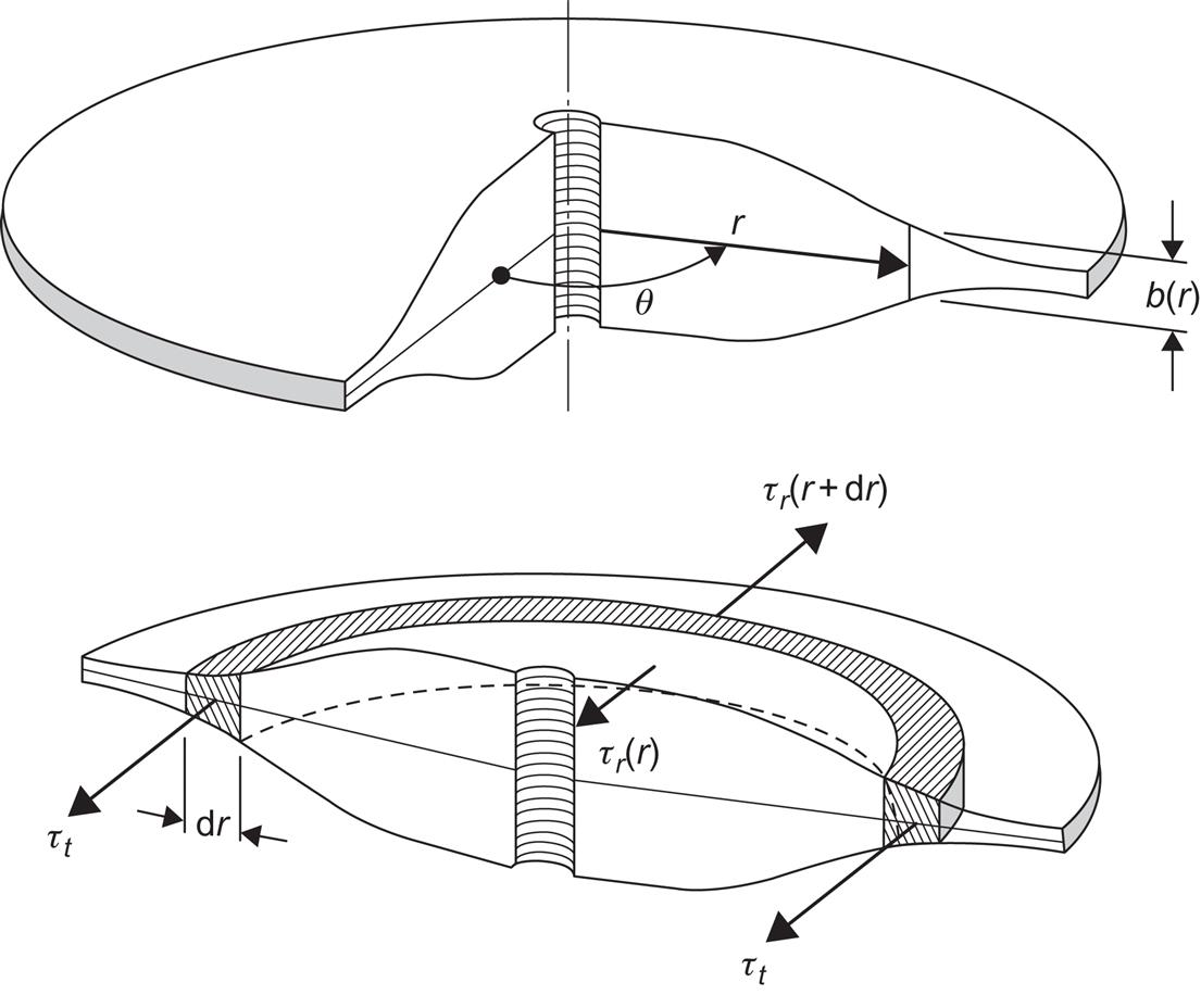
The internal stress forces (5.17) plus any external forces fext determine the acceleration of a small volume of the flywheel situated at the position x:
(5.19)
which is the Newtonian equation of motion. Integrated over some volume V, the force becomes
(5.20)
where in the last line the volume integral over V has been transformed into a surface integral over the surface A enclosing the volume V, with n being a unit vector normal to the surface.
5.5.2 The constant-stress disk
For uniform rotation with constant angular velocity ω, the acceleration on the left-hand side of (5.19) is radial and given by rω2 at the distance r from the axis. Disregarding gravitational forces, the centrifugal force alone must be balanced by the internal stresses, and one may proceed to find the conditions under which all parts of the material experience the same stress τ. If τ equals the tensile strength σ or a specified fraction of it (in order to have a safety margin, as one always would in practice), then the material is utilized optimally, and the energy stored is the maximum that can be achieved using the given material properties.
Taking the volume V as that enclosed between the radius r and r+dr and between the center angle θ=–x/2 and θ=x/2, with the full widths being b(r) and b(r + dr), the balance between the centrifugal force and the internal stresses is obtained from (5.19) and (5.20),
(5.21)
The factors 2 come from the angular integrals over cos θ. The first two terms on the right-hand side of (5.21) are derived from the radial stresses, while the last term represents the tangential stresses on the cuts halving the torus shape considered (cf. Fig. 5.16). To first order in dr, (5.21) may be rewritten as
(5.22)
from which the disc thickness leading to constant stress is found as
(5.23)
The optimal shape is seen to be an infinitely extending disc of exponentially declining thickness.
5.5.3 Other flywheel shapes
The approach used above may be generalized. Instead of assuming constant stress, the shape of the flywheel is assumed [i.e., b(r) is known, the material still being homogeneous and the shape symmetrical around the axis of rotation as well as upon reflection in the midway plane perpendicular to the axis].
Then the stresses will have to be calculated as a function of rotational speed ω. Owing to the assumptions made, there are only two radially varying stress functions to consider, the radial stress τr(r) and the tangential stress τt(r), both depending only on the distance r from the axis of rotation. Stress components parallel to the axis of rotation are considered absent. Considering again a half-torus shape (see Fig. 5.17), the forces perpendicular to the cut plane may be written in a generalization of (5.21):
(5.24)
To first order in dr, this gives, after rearrangement,
(5.25)
This equation relates radial and tangential stresses. In order to determine the stresses, a second relation must be established. This is the relation between stresses and strains, corresponding to Hooke’s law in the theory of elasticity. Introduce deformation parameters εt and εr for tangential and radial stretching by the relations
(5.26)
(5.27)
where (5.26) gives the tangential elongation of the half-torus confined between r and r + dr (see Fig. 5.17), and (5.27) gives the implied radial stretching. Then the stress–strain relations may be written
(5.28)
(5.29)
where the strength of compression Y is called Young’s module and μ is Poisson’s ratio, being the ratio between Y and the corresponding quantity Z measuring the strength of expansion in directions perpendicular to the compression (Shigley, 1972). Eliminating the deformations from (5.27)–(5.29), a new relation between the stresses is obtained:
(5.30)