Search in book...
Toggle Font Controls
Create new playlist

Name your new playlist

Playlist description (optional)
Sign In

Email address

Password

Forgot Password?

or

Continue with Facebook

Continue with Google
Sign Up

Full Name

Email address

Confirm Email Address

Password

or

Continue with Facebook

Continue with Google

Individual renewable energy sources

Abstract

Details characterizing each renewable energy source are presented. For direct solar energy, variability, wavelength spectra and atmospheric scattering, and other processes are discussed. For wind energy, formation and variability is discussed, as well as the distinction between wind velocity, energy, and power. Waterflows in rivers and ocean are discussed, including currents, waves, and tides. Photosynthesis and biological productivity is discussed, and so are a number of other energy flows, such as geothermal, nuclear, or those formed by thermal and salinity gradients.

Keywords

Solar radiation variability; Wind power variability; Ocean currents; Hydropower; Wave power; Tidal power; Geothermal energy; Thermal gradients; Nuclear energy; Biological energy; Biomass productivity

3.1 Direct solar energy

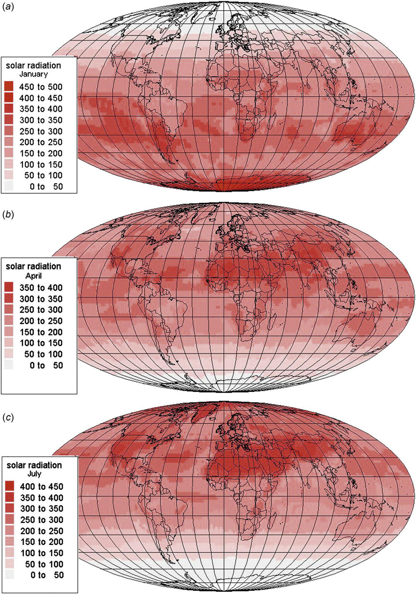
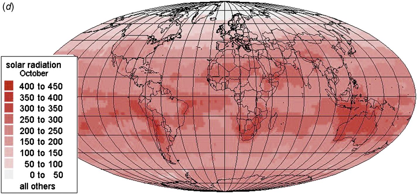
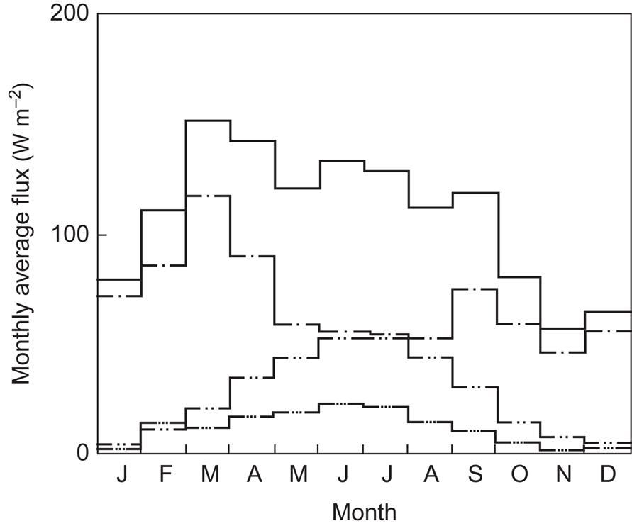
Assessment of the “magnitude” of solar radiation as an energy source will depend on the geographical location, including local conditions, such as cloudiness, turbidity, etc. In section 2.2.2 a number of features of the radiation flux at a horizontal plane are described, such as spectral distribution, direct and scattered parts, geographical variations, and dependence on time, from annual to diurnal variations at a given location. The seasonal variation in solar radiation on a horizontal plane is shown in Fig. 3.1, corresponding to the annual average of Fig. 2.24.

Figure 3.1 Average short-wavelength solar radiation on a horizontal plane at the Earth’s surface (W m⁻²), for the months of January (a), April (b) and July (c) of 1997 (NCEP-NCAR, 1998). (d) Average short-wavelength solar radiation on a horizontal plane at the Earth’s surface (W m⁻²), for the month of October of 1997 (NCEP-NCAR, 1998).

For actual applications, it is often necessary to estimate the amount of radiation received by tilted or complexly shaped devices, and it is useful to look at relations that allow relevant information to be extracted from some basic measured quantities. For instance, radiation data often exist only for a horizontal plane, and a relation is therefore needed to predict the radiation flux on an arbitrarily inclined surface. In regions at high latitudes, directing solar devices toward the Equator at fairly high tilt angles actually gives an increase in incident energy relative to horizontally placed collectors.

Only the incoming radiation is discussed in detail in this section, since the outgoing flux may be modified by the specific type of energy conversion device considered. In fact, such a modification is usually the very idea of the device. A description of some individual solar conversion devices is taken up in Chapter 4, and their potential yield in Chapter 6, in terms of combined demand and supply scenarios.

3.1.1 Direct radiation

The inclination of a surface, e.g., a plane of unit area, may be described by two angles. The tilt angle, s, is the angle between vertical (zenith) and the normal to the surface, and the azimuth angle, γ, is the angle between the southward direction and the direction of the projection of the normal to the surface onto the horizontal plane; γ is considered positive toward east [in analogy to the hour angle]. In analogy to the expression at the top of the atmosphere, given in section 2.2.1, the amount of direct radiation reaching the inclined surface characterized by (s, γ) may be written

$D_{s, γ} = S_{N} \cos θ,$ $D_{s, γ} = S_{N} \cos θ,$ (3.1)

(3.1)

where S_N is the “normal radiation,” i.e., the solar radiation from the direction to the Sun. The normal radiation is entirely direct radiation, according to the definition of direct and scattered radiation given in section 2.2.2. The angle θ is the angle between the direction to the Sun and the normal to the surface specified by s and γ. The geometrical relation between θ and the time-dependent co-ordinates of the Sun, declination δ (2.9) and hour angle ω (2.10), is

$\cos θ = (S C - C S C) \sin + (S S \sin ω + (C C + S S C) \cos ω) \cos δ,$ $\cos θ = (S C - C S C) \sin + (S S \sin ω + (C C + S S C) \cos ω) \cos δ,$ (3.2)

(3.2)

where the time-independent constants are given in terms of the latitude ϕ and the parameters (s, γ) specifying the inclination of the surface,

$\begin{array}{l} S C = \sin ϕ \cos s, \\ C S C = \cos ϕ \sin s \cos γ, \\ S S = \sin s \sin γ, \\ C C = \cos ϕ \cos s, \\ S S C = \sin ϕ \sin s \cos γ . \end{array}$ $\begin{array}{l} S C = \sin ϕ \cos s, \\ C S C = \cos ϕ \sin s \cos γ, \\ S S = \sin s \sin γ, \\ C C = \cos ϕ \cos s, \\ S S C = \sin ϕ \sin s \cos γ . \end{array}$ (3.3)

(3.3)

For a horizontal surface (s=0), θ equals the zenith angle z of the Sun, and (3.2) reduces to the expression for cos z given in section 2.2.1. Instead of describing the direction to the Sun by δ and ω, the solar altitude h=1/2π−z and azimuth Az (conventionally measured as positive toward the west, in contrast to the hour angle) may be introduced. The two sets of co-ordinates are related by

$\begin{array}{l} \sin h = \sin δ \sin ϕ + \cos δ \cos ϕ \cos ω, \\ \sin A z \cos h = - \cos δ \sin ω . \end{array}$ $\begin{array}{l} \sin h = \sin δ \sin ϕ + \cos δ \cos ϕ \cos ω, \\ \sin A z \cos h = - \cos δ \sin ω . \end{array}$ (3.4)

(3.4)

In the height–azimuth co-ordinate system, (3.2) may be written

$\cos θ = \sin h \cos s + \cos h \sin s \cos (A z + γ) .$ $\cos θ = \sin h \cos s + \cos h \sin s \cos (A z + γ) .$ (3.5)

(3.5)

Again, the sign conventions for Az and γ are opposite, so that the argument of the last cosine factor in (3.5) is really the difference between the azimuth of the Sun and the projection of the normal to the surface considered. If cos θ found from (3.2) or (3.5) is negative, it means that the Sun is shining on the “rear” side of the surface considered. Usually, the surface is to be regarded as “one-sided,” and cos θ may then be replaced by zero, whenever it assumes a negative value, in order that the calculated radiation flux (3.1) becomes properly zero.

If data giving the direct radiation flux D on a horizontal plane are available, and the direct flux impinging on an inclined surface is wanted, the above relations imply that

$D_{s, γ} = D \cos θ / \cos z .$ $D_{s, γ} = D \cos θ / \cos z .$

It is evident that care should be taken in applying this relation when the Sun is near the horizon.

More reliable radiation fluxes may be obtained if the normal incidence radiation flux S_N is measured (as function of time) and (3.1) is used directly. S_N is itself a function of zenith distance z, as well as a function of the state of the atmosphere, including ozone mixing ratio, water vapor mixing ratio, aerosol and dust content, and cloud cover. The dependence on zenith angle is primarily a question of the path that the radiation has taken through the atmosphere. This path-length is shortest when the Sun is in zenith (often denoted air mass one for a clear sky) and increases with z, being quite large when the Sun is near the horizon and the path is curved due to diffraction. The extinction in the atmosphere is normally reduced at elevated locations (or low-pressure regions, notably mountain areas), in which case the effective air mass may become less than one. Figure 3.2 gives some typical variations of S_N with zenith angle for zero, small, and heavy particle load (turbidity). Underlying assumptions are: cloudless sky, water vapor content throughout a vertical column equal to 0.02 m³ m⁻², standard sea-level pressure, and mean distance to the Sun (Robinson, 1966).

Figure 3.2 Normal incidence radiation as a function of zenith angle for a cloudless sky with different particle contents: (a) hypothetical atmosphere with zero turbidity [B=0, no aerosols but still water vapor and molecular (Rayleigh) scattering]; (b), clear sky (B=0.01); (c), atmosphere with heavy aerosol pollution (B=0.4). B is the turbidity coefficient B_λ (defined in the text) averaged over wavelengths. Sea-level pressure (10⁵ N m⁻²), a water content of 0.02 m³ m⁻², an ozone content of 0.0034 m³ m⁻² (both referred to standard temperature and pressure) and mean Earth–Sun distance have been assumed. At the top, an approximate air mass scale is provided, relative to the one for a vertical path from sea level. Based on Robinson (1966).

Since a complete knowledge of the state of the atmosphere is needed in order to calculate S_N, such a calculation would have to be coupled to the equations of state and motion discussed in section 2.3.1. Only some average behavior may be described without doing this, and if, for example, hourly values of S_N are required in order to predict the performance of a particular solar energy conversion device, it would be better to use measured values of S_N (which are becoming available for selected locations throughout the world, cf. Turner, 1974) or values deduced from measurements for horizontal surfaces. Measurement techniques are discussed by Coulson (1975), among others.

Attempts to parameterize the solar radiation received at the ground are usually made for global radiation (direct plus scattered, and, for tilted planes, radiation reflected onto the surface), rather than separately for normal incidence and scattered radiation [cf. (2.20)].

3.1.1.1 Dependence on turbidity and cloud cover

The variability of S_N due to turbidity may be demonstrated by noting the range of S_N values implied by extreme high or low turbidities, in Fig. 3.2, and by considering the spread in mean daily turbidity values, an example of which is shown in Fig. 3.3. The turbidity coefficient B_λ for a given wavelength may be defined through an attenuation expression of the form

$S_{N} (λ) / E_{0 +}^{s w} (λ) = 10^{- m_{r} (τ_{λ}^{s} + τ_{λ}^{a} + B_{λ})} .$ $S_{N} (λ) / E_{0 +}^{s w} (λ) = 10^{- m_{r} (τ_{λ}^{s} + τ_{λ}^{a} + B_{λ})} .$

Figure 3.3 Turbidity coefficient B_λ at the wavelength λ=5×10⁻⁷ m, as measured during 1972 at Raleigh (North Carolina) by Bilton *et al*. (1974). Daily means are indicated by *dots*, monthly means by the *curve*. Only days with a cloudless sky in the direction of the Sun have been included. Data points above B_λ=0.4 are indicated at 0.4 (cf. the high turbidity curve of Fig. 3.2).

Here m_r is the relative air mass (optical path-length in the atmosphere), $τ_{λ}^{s}$ $τ_{λ}^{s}$ describes the scattering on air molecules, and $τ_{λ}^{a}$ $τ_{λ}^{a}$ is the absorption by ozone. In terms of the cross-sections σ_s(λ), σ_a(λ), and σ_p(λ) for scattering on air molecules, ozone absorption, and attenuation by particles, one has

$- m_{r} τ_{λ}^{s} = \log_{10} {\exp (\int σ_{s} (λ) d s)},$ $- m_{r} τ_{λ}^{s} = \log_{10} {\exp (\int σ_{s} (λ) d s)},$

and similarly for $τ_{λ}^{a}$ $τ_{λ}^{a}$ and B_λ. Figure 3.3 gives both daily and monthly means for the year 1972 and for a wavelength of 5×10⁻⁷ m (Bilton et al., 1974). The data suggest that it is unlikely to be possible to find simple, analytical expressions for the detailed variation of the turbidity or for the solar fluxes, which depend on turbidity.

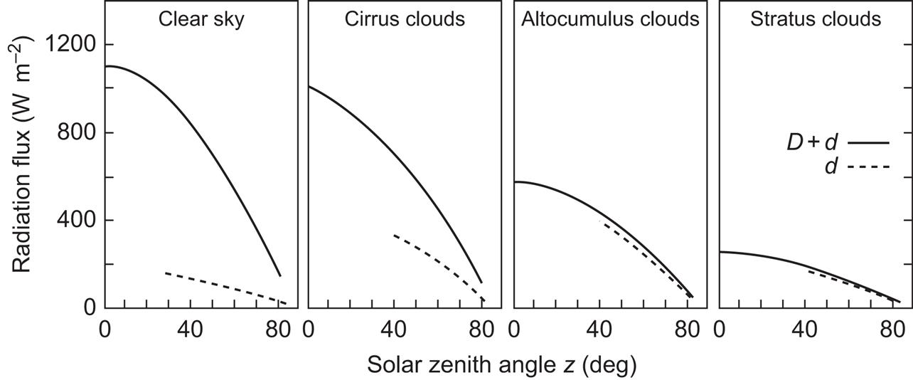
Another major factor determining the amount and distribution of different types of fluxes is the cloud cover. Both cloud distribution and cloud type are important. For direct radiation flux, the important questions are whether the path-line is obscured, and, if it is, how much attenuation is caused by the particular type of cloud. Figure 3.4 shows the total and scattered flux on a horizontal plane (and, by subtraction, the direct flux), for a clear sky and three different types of clouds, as a function of the zenith angle of the Sun. The cloud classification represents only a general indication of category. It is evident in this example that altocumulus and stratus clouds are almost entirely impermeable to direct radiation, whereas cirrus clouds allow the penetration of roughly half the direct radiation flux. Meteorological observations containing records of sunshine (indicating whether the direction to the Sun is obscured) and of cloud cover (as a percentage and identifying the cloud types and their estimated height) may allow a fairly reliable estimate of the fraction of direct radiation reaching a plane of given orientation.

Figure 3.4 The influence of clouds on the radiation flux reaching a horizontal plane (total short-wavelength flux, *D+d*, and scattered flux alone, d). Based on measurements by J. Millard and J. Arvesen, as quoted in Turner (1974).

3.1.2 Scattered radiation

The scattered radiation for a clear sky may be estimated from knowledge of the composition of the atmosphere, as described in section 2.3.1. The addition of radiation scattered from clouds requires knowledge of the distribution and type of clouds, and the accuracy with which a calculation of the scattered flux on a given plane can be made is rather limited. Even with a clear sky, the agreement between calculated and observed fluxes is not absolute, as seen, for example, in Fig. 2.41.

Assuming that the distribution of intensity, $S_{h, A z}^{s c a t t .},$ $S_{h, A z}^{s c a t t .},$ for scattered radiation as a function of the directional co-ordinates (h, Az) [or (δ, ω)] is known, then the total flux of scattered radiation reaching a plane tilted at an angle s and directed azimuthally, at an angle γ away from south, may be written

$d_{s, λ} = \int S_{h, A z}^{s c a t t .} \cos θ d Ω = \int_{0}^{π / 2} d (A z) \int_{h_{\min} (A z)}^{π / 2} d h S_{h, A z}^{s c a t t .} \cos θ (h, A z) \cos h .$ $d_{s, λ} = \int S_{h, A z}^{s c a t t .} \cos θ d Ω = \int_{0}^{π / 2} d (A z) \int_{h_{\min} (A z)}^{π / 2} d h S_{h, A z}^{s c a t t .} \cos θ (h, A z) \cos h .$ (3.6)

(3.6)

Here h_min(Az) is the smallest height angle, for a given azimuth, for which the direction defined by (h, Az) is on the “front” side of the inclined plane. The unit solid angle is dΩ=sin z dz d(Az)=–cos h dh d(Az). For a horizontal plane θ (h, Az)=z=1/2π–h.

If the scattered radiation is isotropic,

$S_{h, A z}^{s c a t t .} = c o n s t a n t = S^{s c a t t .},$ $S_{h, A z}^{s c a t t .} = c o n s t a n t = S^{s c a t t .},$

then the scattered radiation flux on a horizontal plane becomes

$d = π S^{s c a t t .},$ $d = π S^{s c a t t .},$ (3.7)

(3.7)

and the scattered radiation flux on an arbitrarily inclined surface may be written

$d_{s, γ} = d \cos^{2} (s / 2),$ $d_{s, γ} = d \cos^{2} (s / 2),$ (3.8)

(3.8)

an expression that can also be derived by considering the fraction of the sky “seen” by the tilted surface.

A realistic distribution of scattered radiation intensity is not isotropic, and, as mentioned earlier, it is not even constant for a cloudless sky and fixed position of the Sun, but depends on the momentary state of the atmosphere. Figure 3.5 shows the result of measurements for a cloudless sky (Kondratyev and Fedorova, 1976), indicating that the assumption of isotropy would be particularly poor for planes inclined directly toward or away from the Sun (Az equal to 0 or π relative to the solar azimuth). Robinson (1966) notes, from observations such as the one shown in Fig. 2.41, that the main differences between observed distributions of scattered radiation and an isotropic one are: (a) increased intensity for directions close to that of the Sun, and (b) increased intensity near the horizon. In particular, the increased intensity in directions near the Sun is very pronounced, as is also evident from Fig. 3.5, and Robinson suggests that about 25% of d, the scattered radiation on a horizontal plane, should be subtracted from d and added to the direct radiation, before the calculation of scattered radiation on an inclined surface is performed using the isotropic model. However, such a prescription would not be generally valid, because the increased intensity in directions near the Sun is a function of the turbidity of the atmosphere as well as of cloud cover.

Figure 3.5 Ratio between scattered radiation flux on an inclined surface (tilt angle s, azimuth angle γ) and scattered radiation flux on a horizontal surface for a cloudless sky with solar height 15°. Based on Kondratyev and Fedorova (1976).

It is evident from Fig. 3.4 that the effect of clouds generally is to diminish direct radiation and increase scattered radiation, although not in the same proportion. Cirrus clouds and, in particular, altocumulus clouds substantially increase the scattered flux on a horizontal plane.

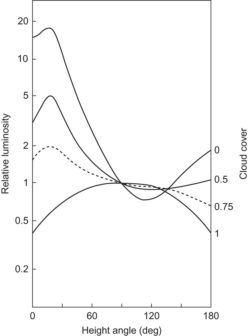
The radiation scattered by clouds is not isotropically distributed. Figure 3.6 gives the luminance distribution, i.e., the intensity of total radiation, along the great circle containing zenith as well as the direction to the Sun, the height angle of which was 20° at the time of measurement. For complete cloud cover, the luminance distribution is entirely due to scattered radiation from the clouds, and it is seen to be maximum at zenith and falling to 0.4 times the zenith value at the horizon.

Figure 3.6 Luminance distribution along a great circle containing zenith as well as the direction toward the Sun, as a function of cloud cover. The distributions have been normalized at h=90°. The data are based on several measurements with solar height 20° and mean turbidity, performed by Tonne and Normann (1960).

3.1.3 Total short-wavelength radiation

For inclined surfaces or surfaces surrounded by elevated structures, the total short-wavelength (wavelengths below, say, 3×10⁻⁶ m) radiation flux comprises not only direct and scattered radiation, but also radiation reflected from the ground or from the surroundings onto the surface considered.

3.1.3.1 Reflected radiation

The reflected radiation from a given area of the surroundings may be described in terms of an intensity distribution, which depends on the physical nature of the area in question, as well as on the incoming radiation on that area. If the area is specularly reflecting, and the incoming radiation is from a single direction, then there is also a single direction of outgoing, reflected radiation, a direction that may be calculated from the law of specular reflection (polar angle unchanged, azimuth angle changed by π). Whether the reflection is specular may depend not only on the fixed properties of the particular area, but also on the wavelength and polarization of the incoming radiation.

The extreme opposite of specular reflection is completely diffuse reflection, for which by definition the reflected intensity is isotropic over the hemisphere bordered by the plane tangential to the surface at the point considered, no matter what the distribution of incoming intensity. The total (hemispherical) amount of reflected radiation is in this case equal to the total incoming radiation flux times the albedo a of the area in question,

$R = a E_{+},$ $R = a E_{+},$

where, for horizontal surfaces, E₊=D+d (for short-wavelength radiation).

In general, the reflection is neither completely specular nor completely diffuse. In this case, the reflected intensity in a given direction, e.g., specified by height angle and azimuth, $S_{Ω_{r}}^{r e f l .},$ $S_{Ω_{r}}^{r e f l .},$ depends on the distribution of incident radiation intensities $S_{Ω_{r}}^{i n c .}$ $S_{Ω_{r}}^{i n c .}$ ,*

$S_{Ω_{r}}^{r e f l .} = \int_{h e m i s p h e r e} ρ_{2} (Ω_{r}, Ω_{i}) S_{Ω_{i}}^{i n c .} \cos θ (Ω_{i}) d Ω_{i} .$ $S_{Ω_{r}}^{r e f l .} = \int_{h e m i s p h e r e} ρ_{2} (Ω_{r}, Ω_{i}) S_{Ω_{i}}^{i n c .} \cos θ (Ω_{i}) d Ω_{i} .$ (3.9)

(3.9)

Here ρ₂(Ω_y, Ω_i) is called the bi-angular reflectance (Duffie and Beckman, 1974; these authors include an extra factor π in the definition of ρ₂). Dividing by the average incoming intensity,

$\int S_{Ω_{i}}^{i n c .} \cos θ (Ω_{i}) d Ω_{i} \int \cos θ (Ω_{i}) d Ω_{i} = E_{+} / π$ $\int S_{Ω_{i}}^{i n c .} \cos θ (Ω_{i}) d Ω_{i} \int \cos θ (Ω_{i}) d Ω_{i} = E_{+} / π$

a reflectance depending only on one set of angles (of reflected radiation) is defined,

$ρ_{1} (Ω r) = π S_{Ω_{r}}^{r e f l .} / E_{+ .}$ $ρ_{1} (Ω r) = π S_{Ω_{r}}^{r e f l .} / E_{+ .}$ (3.10)

(3.10)

In general, ρ₁ is not a property of the reflecting surface, since it depends on incoming radiation, but if the incoming radiation is isotropic (diffuse or blackbody radiation), the incoming intensity can be divided out in (3.10).

The total hemispherical flux of reflected radiation may be found by integration of (3.9),

$R = \int_{h e m i s p h e r e} S_{Ω_{r}}^{r e f l .} \cos θ (Ω_{r}) d Ω_{r},$ $R = \int_{h e m i s p h e r e} S_{Ω_{r}}^{r e f l .} \cos θ (Ω_{r}) d Ω_{r},$ (3.11)

(3.11)

and the corresponding hemispherical reflectance,

$ρ = R / E_{+} = a,$ $ρ = R / E_{+} = a,$ (3.12)

(3.12)

is equal to the albedo defined above.

All of the above relations have been written without reference to wavelength, but they are valid for each wavelength λ, as well as for appropriately integrated quantities.

In considering the amount of reflected radiation reaching an inclined surface, the surrounding surfaces capable of reflecting radiation are often approximated by an infinite, horizontal plane. If the reflected radiation is further assumed to be isotropic of intensity S^refl., then the reflected radiation flux received by the inclined surface is

$R_{s, γ} = π S^{r e f l .} \sin^{2} (s / 2) .$ $R_{s, γ} = π S^{r e f l .} \sin^{2} (s / 2) .$ (3.13)

(3.13)

The factor sin²(s/2) represents the fraction of the hemisphere above the inclined surface from which reflected radiation is received. This fraction is evidently complementary to the fraction of the hemisphere from which scattered radiation is received and, therefore, equal to 1−cos²(s/2) from (3.8). The albedo (3.12) may be introduced, noting from (3.11) that R=πS^refl. for isotropic reflection,

$R_{s, γ} = a E_{+} \sin^{2} (s / 2) .$ $R_{s, γ} = a E_{+} \sin^{2} (s / 2) .$ (3.14)

(3.14)

For short-wavelength radiation, the flux E₊ on a horizontal plane equals D+d, the sum of direct and scattered short-wavelength fluxes.

If the geometry of the reflecting surroundings is more complicated (than a plane), or if the reflected intensity is not isotropic, the calculation of the amount of reflected radiation reaching a given inclined surface involves integration over the hemisphere seen by the inclined surface. Thus, for each direction of light reflected onto the inclined plane, a contribution to $S_{Ω_{r}}^{r e f l .}$ $S_{Ω_{r}}^{r e f l .}$ is included from the first unobscured point on the line of sight capable of reflecting radiation. If semitransparent objects (such as a water basin) are present in the surroundings, the integration becomes three-dimensional, and the refraction and transmission properties of the partly opaque objects must be considered.

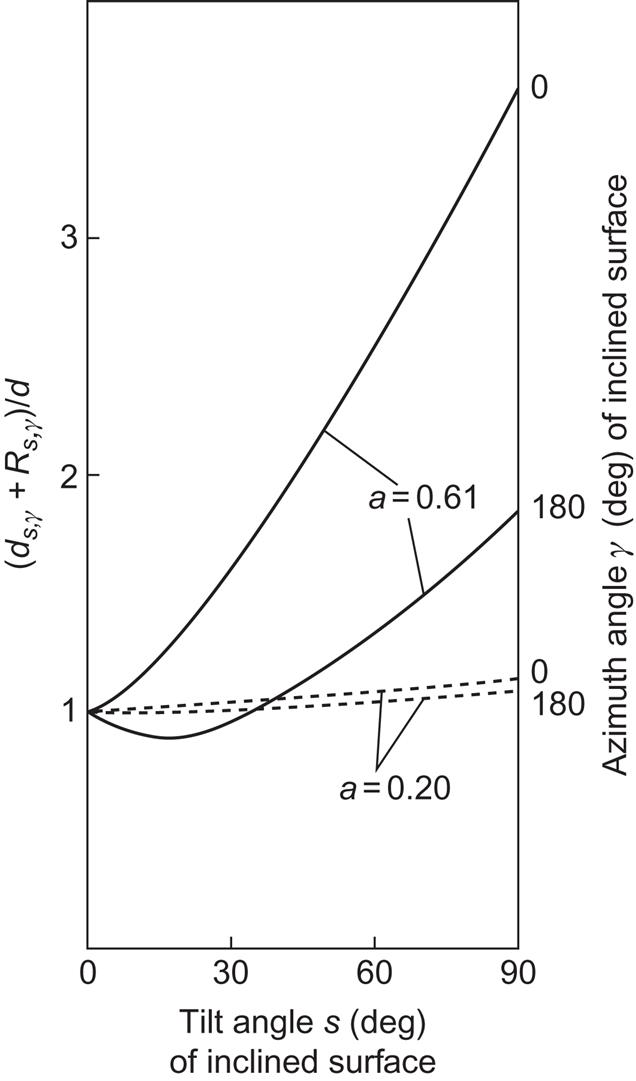
Figure 3.7 shows an example of the enhancement of indirect radiation that may result from increasing albedo of the surroundings—in this case, due to snow cover in winter (Kondratyev and Fedorova, 1976). The rejected radiation on the inclined surface reaches a maximum value for the tilt angle s=90° (vertical).

Figure 3.7 The ratio of scattered plus reflected radiation flux on inclined surfaces to that on a horizontal surface (scattered flux d only) for a clear sky with the Sun at height 34°. Measurements corresponding to two different ground albedos are depicted, based on summer and winter (snow-covered ground) conditions at a location in the Soviet Union (Kondratyev and Fedorova, 1976).

3.1.3.2 Average behavior of total short-wavelength radiation

The sum of direct, scattered, and reflected radiation fluxes constitutes the total short-wavelength (sw) radiation flux. The total short-wavelength flux on a horizontal surface is sometimes referred to as the global radiation, i.e., D+d (if there are no elevated structures to reflect radiation onto the horizontal surface). For an inclined surface of tilt angle s and azimuth γ, the total short-wavelength flux may be written

$E_{s, γ}^{s w} = D_{s, γ} + d_{s, γ} + R_{s, γ},$ $E_{s, γ}^{s w} = D_{s, γ} + d_{s, γ} + R_{s, γ},$ (3.15)

(3.15)

with the components given by (3.1), (3.6) or (3.8), and (3.14) or a generalization of it. The subscript “+” on E^sw has been left out, since the direction of the flux is clear from the values of s and γ (the E₋ flux would generally require s>90°).

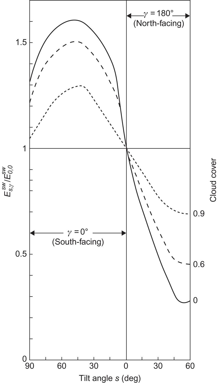
Examples of the influence of clouds, and of solar zenith angle, on global radiation $E_{s = 0, γ}^{s w}$ $E_{s = 0, γ}^{s w}$ are given in Fig. 3.4. Figure 3.8 illustrates the influence of cloud cover on the daily sum of total short-wavelength radiation received by inclined surfaces, relative to that received by a horizontal surface. For south-facing slopes, the radiation decreases with increasing cloud cover, but for north-facing slopes the opposite takes place.

Figure 3.8 Daily sums of total short-wavelength radiation on an inclined plane, relative to that of a horizontal plane, for different cloud cover and as a function of tilt angle for north- and south-facing surfaces. Based on measurements in the Soviet Union, Kondratyev and Fedorova (1976).

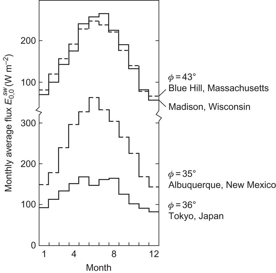
Monthly averages of total short-wavelength radiation for different geographical locations are shown in Figs. 3.9 and 3.10 for a horizontal surface. In Fig. 3.10, two sets of data are compared, each representing a pair of locations with the same latitude. The two at ϕ≈43°N correspond to a coastal and a continental site, but the radiation, averaged for each month, is nearly the same. The other pair of locations are at 35°–36°N. Albuquerque has a desert climate, while Tokyo is near the ocean. Here the radiation patterns are vastly different during summer, by as much as a factor of two. The summer solar radiation in Tokyo is also smaller than in both the 43°N sites, presumably due to the influence of urbanization (cf. section 2.4.2) and a high natural frequency of cloud coverage. Other average properties of radiation fluxes on horizontal surfaces are considered in section 2.2.2, notably for a latitude 53°N location.

Figure 3.9 Smoothed variation with seasons of the average daily flux (24-h average) of total short-wavelength radiation on a horizontal plane for selected geographical locations. Based on Flack and Morikofer (1964).

Figure 3.10 Monthly average flux on a horizontal plane for pairs of locations with similar latitude but different climate. Based on data from NOAA (U.S. National Oceanic and Atmospheric Administration), quoted from Duffie and Beckman (1974).

Looking more closely at some specific cases, Fig. 3.11 shows the total short-wavelength radiation on a vertical plane facing south, west, east, and north for a location at ϕ=56°N. The monthly means have been calculated from the hourly data of the Danish reference year (Andersen et al., 1974), using the isotropic approximation (3.8) and (3.14) with an assumed albedo a=0.2. The Danish reference year consists of selected meteorological data exhibiting “typical” fluctuations. This is achieved by selecting monthly sequences of actual data, with monthly averages of each of the meteorological variables in the vicinity of the 30-year mean. The different sequences that make up the reference year have been taken from different years. The variables pertaining to solar radiation are global radiation (D+d), normal-incidence radiation (S_N), and scattered radiation on a horizontal plane (d). Only global radiation has been measured over extended periods of time, but the two other variables have been constructed so that the three variables, of which only two are independent, become reasonably consistent. Several other countries are in the process of constructing similar reference years, which will allow for easy comparison of, for example, performance calculations of solar energy devices or building insulation prescriptions. Monthly averages of the basic data of the Danish reference year, D+d and D, are shown in Fig. 3.12. Reference years have subsequently been constructed for a number of other locations (European Commission, 1985).

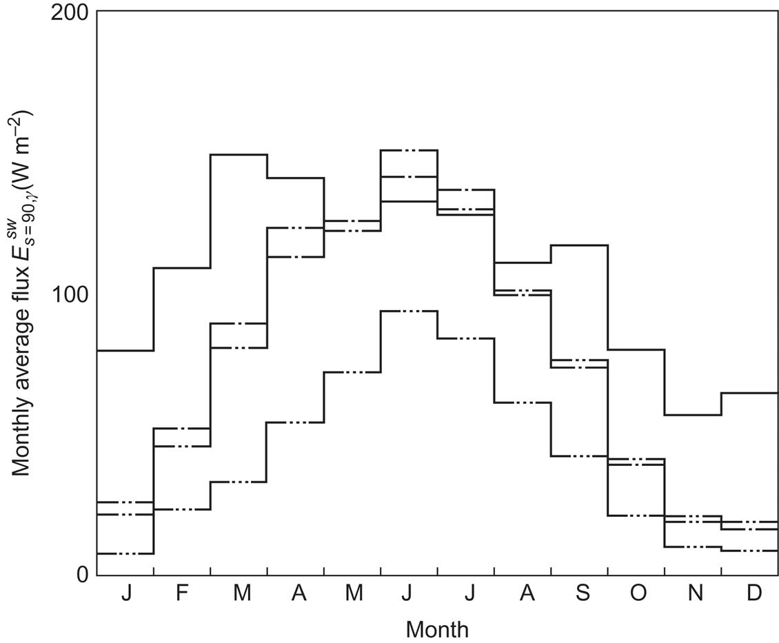
Figure 3.11 Monthly average flux on a vertical surface with different azimuthal orientations, based on the Danish reference year (latitude 56°) and an assumed ground albedo of 0.2 (0.9 with snow cover). Key: ––––– γ=0° (south); –⋅–⋅– γ=–90° (west); –⋅⋅–⋅⋅– γ=90° (east); –⋅⋅⋅–⋅⋅⋅– γ=180° (north). This and the following calculations assume that the scattered radiation is isotropic.

Figure 3.12 Monthly average short-wavelength flux on horizontal surface, and the direct part, D, based on the Danish reference year, ϕ=56°N (Andersen *et al*., 1974).

Figure 3.13 shows the composition of the total short-wavelength flux on a vertical, south-facing surface, in terms of direct, scattered, and reflected radiation. It has been assumed that the albedo changes from 0.2 to 0.9 when the ground is covered by snow (a piece of information also furnished by the reference year). Snow cover is therefore responsible for the relative maximum in reflected flux for February. The proportion of direct radiation is substantially higher during winter for this vertical surface than for the horizontal surface (Fig. 3.12).

Figure 3.13 Components of monthly average fluxes on vertical, south-facing surface. Key: –––– total short-wavelength radiation; –⋅–⋅– direct radiation D_s,γ; –⋅⋅–⋅⋅– scattered radiation d_s,γ; –⋅⋅⋅–⋅⋅⋅– reflected radiation R_s,γ (in all cases γ=0). The calculation is based on the Danish reference year, ϕ=56°N, and an assumed albedo of 0.2 (0.9 with snow cover).

3.1.3.3 Inclined surfaces

Since the devices used to capture solar radiation for heat or power production are often flat-plate collectors integrated into building facades or roofs, it is important to be able to estimate energy production for such inclined mountings as function of time and location.

Available satellite solar data comprise only down-going fluxes of total radiation on a horizontal plane at the ground surface level. They are calculated from solar fluxes at the top of the atmosphere and reflected radiation reaching the satellite, with use of measured cloud and turbidity data (ECMWF, 2008). At low latitudes, these may be appropriate for solar devices, but at higher latitudes, radiation on inclined surfaces has to be derived indirectly.

Data for inclined surfaces exist directly for a limited number of local meteorological stations and are incorporated into the so-called “reference data” constructed for the purpose of engineering applications in building construction. As these data are not universally available, I shall instead try to estimate radiation on inclined surfaces from the horizontal ones. This is not a trivial task, because it requires a separation of the total radiation known on a horizontal plane into direct and scattered radiation, which must be treated differently: the direct radiation can be transformed to that on inclined surfaces by a set of geometrical calculations given above, but it is rarely known precisely how much of the total radiation is scattered, as this depends on many elusive parameters (solar height, attenuation in the air, absorption and reflection on clouds of different kinds). These same factors influence the radiation on a plane of some particular inclination, but differently and in a way that varies with time. Thus one can only hope to describe some average behavior without performing additional measurements.

The following procedure was used to estimate radiation on south-facing planes tilted at 45°S and 90°S: 62.5% of the horizontal radiation, representing direct as well as nearly forward-scattered radiation (i.e., radiation scattered by small angles, known to be a large component of the indirect radiation) is treated by the straightforward angular transformations to normal-incidence radiation, and then to radiation on the tilted surface. Strictly direct radiation is roughly 50% (see above), so 25% of the scattered radiation is assumed to arrive from directions close to that of the Sun. The remaining 37.5% of the horizontal radiation is distributed on the inclined surfaces by multiplication with a factor taken as 1.5 for the s=45° tilted surface and 1.25 for the s=90° tilted surface, based on measurements by Kondratyev and Fedorova (1976). In other words, the scattered radiation is far from isotropic, as this would give a simple cos²(s/2)-factor due to the reduced fraction of the sky seen by the surfaces at a tilt angle s.

The resulting monthly average distribution of radiation for January and July are given in Figs. 3.14 and 3.15 for the Northern hemisphere, using 6-hour data for the year 2000. The average values serve to provide a general overview and the full 6-hour data set is necessary for actual simulation studies. On the Southern hemisphere, appropriate tilt angles for solar collectors would be north-facing rather than south-facing. For those locations where measurements have been performed, the quality of the model can be assessed. Based on only a cursory comparison, the model seems to agree with data at mid-latitudes (i.e., the regions of interest here) and the variations in radiation seem to be generally of an acceptable magnitude. However, deviations could be expected at other latitudes or at locations with particular meteorological circumstances.

Figure 3.14 Estimated January solar radiation in W m⁻² on differently tilted surfaces, calculated from the horizontal data of ECMWF (2008).

Figure 3.15 Estimated July solar radiation in W m⁻² on surfaces of various tilt angles, calculated from the horizontal data of ECMWF (2008).

Looking for comparison at some of the empirical data for inclined surfaces, Fig. 3.16 gives, for a specific location, the variation of the yearly average fluxes with the tilt angle s, still for a south-facing surface (γ=0). The variation of monthly averages of the total flux with tilt angle for a south-facing surface is given in Fig. 3.17.

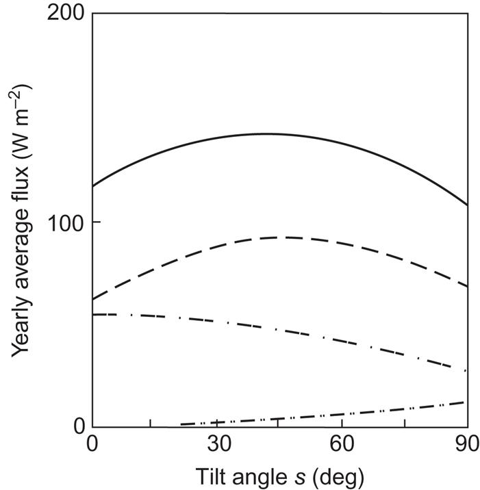
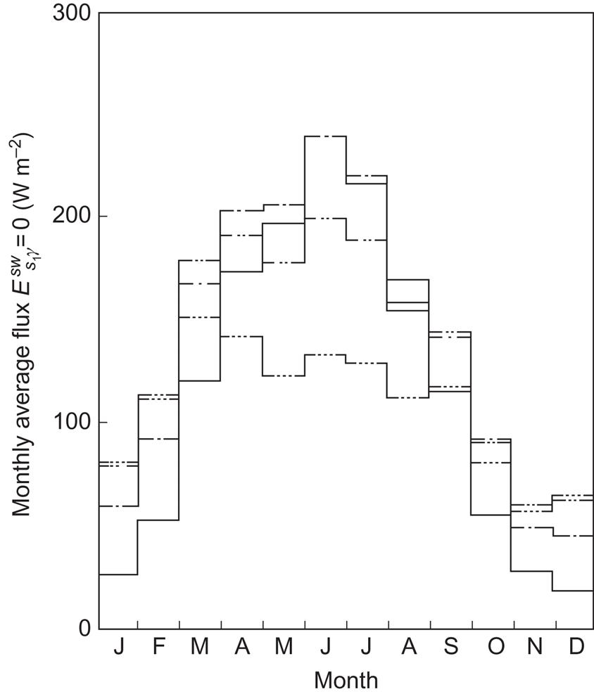
Figure 3.16 Components of yearly average fluxes on a vertical, south-facing surface. Key: –––– total short-wavelength radiation; – – – direct radiation D_s,γ; –⋅–⋅– scattered radiation d_s,γ; –⋅⋅–⋅⋅– reflected radiation R_s,γ (in all cases γ=0). The calculation is based on the Danish reference year, ϕ=56°N, and an assumed albedo of 0.2 (0.9 with snow cover).

Figure 3.17 Monthly average of total short-wavelength radiation on inclined, south- facing surfaces, based on the Danish reference year, ϕ=56° N. Key: –––– tilt angle s=0; –⋅– s=30°; –⋅⋅– s=60°; –⋅⋅⋅– s=90°.

According to Fig. 3.16, the maximum yearly short-wavelength radiation in Denmark (ϕ=56°N) is obtained on a south-facing surface tilted about 40°, but the maximum is broad. The maximum direct average flux is obtained at a tilt angle closer to ϕ, which is clear because at the top of the atmosphere the maximum would be attained for s equal to the latitude plus or minus the Sun’s declination, the extremes of which are about ±23° at summer and winter solstices. From Fig. 3.17, one can see that the most constant radiation over the year is obtained for s=90°. The December maximum value is for s=75°, but the solar radiation on an s=90° surface is only 1%–2% smaller.

3.1.4 Long-wavelength radiation

As suggested by Figs. 2.20 and 2.26, the long-wavelength radiation reaching a plane situated at the Earth’s surface may be quite substantial, in fact, exceeding the short-wavelength radiation when averaged over 24 h. However, the outgoing long-wavelength radiation is (again on average) still larger, so that the net long-wavelength flux is directed away from the surface of the Earth. The ground and most objects at the Earth’s surface emit long-wavelength (lw) radiation approximately as a blackbody, while the long-wavelength radiation from the atmosphere often deviates substantially from any blackbody spectral distribution.

In general, the emission and absorption of radiation by a body may be described by the spectral and directional emittance, ε_λ(Ω), and the corresponding absorptance, α_λ(Ω). These quantities are related to e(ν) and κ(ν) of section 2.1.1, which may also depend on the direction Ω, by

$e (ν, Ω) = ε_{λ} (Ω) d F^{P l a n c k} / d ν, κ (ν, Ω) = α_{λ} (Ω),$ $e (ν, Ω) = ε_{λ} (Ω) d F^{P l a n c k} / d ν, κ (ν, Ω) = α_{λ} (Ω),$

for corresponding values of frequency ν and wavelength λ.

Thus, ε_λ(Ω) is the emission of the body, as a fraction of the blackbody radiation (2.3) for emission in the direction Ω, and α_λ(Ω) is the fraction of incident flux, again from the direction specified by Ω, which is absorbed by the body.

Where a body is in complete thermodynamic equilibrium with its surroundings (or more specifically those with which it exchanges radiation), Kirchhoff’s law is valid (see, e.g., Siegel and Howell, 1972),

$ε_{λ} (Ω) = α_{λ} (Ω) .$ $ε_{λ} (Ω) = α_{λ} (Ω) .$ (3.16)

(3.16)

However, since both ε_λ(Ω) and α_λ(Ω) are properties of the body, they are independent of the surroundings, and hence (3.16) is also valid away from equilibrium. This does not apply if wavelength averages are considered. Then ε(Ω) is still a property of the surface, but α(Ω) depends on the spectral composition of the incoming radiation, as follows from the definition of α(Ω),

$α (Ω) = \int α_{λ} (Ω) S_{λ}^{i n c} (Ω) d λ / \int S_{λ}^{i n c} (Ω) d λ .$ $α (Ω) = \int α_{λ} (Ω) S_{λ}^{i n c} (Ω) d λ / \int S_{λ}^{i n c} (Ω) d λ .$

Further averaging over directions yields the hemispherical emittance ε and absorptance α, the former still being a property of the surface, the latter not.

Consider now a surface of temperature T_s and orientation angles (s, γ), which emit long-wavelength radiation in such a way that the hemispherical energy flux is

$E_{-}^{l w, e m i s s i o n} = ε^{l w} σ {T_{s}}^{4},$ $E_{-}^{l w, e m i s s i o n} = ε^{l w} σ {T_{s}}^{4},$ (3.17)

(3.17)

where σ is Stefan’s constant (5.7×10⁻⁸ W m⁻² K⁻⁴). For pure blackbody radiation from a surface in thermal equilibrium with the temperature T_s (forming an isolated system, e.g., a cavity emitter), ε^lw equals unity.

The assumption that ε_λ=ε (emissivity independent of wavelength) is referred to as the gray-body assumption. It implies that the energy absorbed from the environment can be described by a single absorptivity α^lw=ε^lw. Further, if the long-wavelength radiation from the environment is described as blackbody radiation corresponding to an effective temperature T_e, the incoming radiation absorbed by the surface may be written

$E_{+}^{l w, a b s .} = ε^{l w} σ {T_{e}}^{4} .$ $E_{+}^{l w, a b s .} = ε^{l w} σ {T_{e}}^{4} .$ (3.18)

(3.18)

If the part of the environmental flux reflected by the surface is denoted R(=ρ^lw σT_e⁴), then the total incoming long-wavelength radiation flux is $E_{+}^{l w} = R + E_{+}^{l w, a b s .},$ $E_{+}^{l w} = R + E_{+}^{l w, a b s .},$ and the total outgoing flux is $E_{-}^{l w} = R + E_{-}^{l w, e m i s s i o n},$ $E_{-}^{l w} = R + E_{-}^{l w, e m i s s i o n},$ and thus the net long-wavelength flux is

$E^{l w} = ε^{l w} σ ({T_{e}}^{4} - {T_{s}}^{4}) .$ $E^{l w} = ε^{l w} σ ({T_{e}}^{4} - {T_{s}}^{4}) .$ (3.19)

(3.19)

The reflection from the environment of temperature T_e back onto the surface of temperature T_s has not been considered, implying an assumption regarding the “smallness” of the surface considered as compared with the effective surface of the environment. Most surfaces that may be contemplated at the surface of the Earth (water, ice, grass, clay, glass, concrete, paints, etc.) have long-wavelength emissivities ε^lw close to unity (typically about 0.95). Materials like iron and aluminum with non-polished surfaces have low long-wavelength emissivities (about 0.2), but often their temperature T_s is higher than the average temperature at the Earth’s surface (due to high absorptivity for short-wavelength radiation), so that (3.19) may still be a fair approximation, if T_s is chosen as an average temperature of physical surfaces. If the surface is part of an energy-collecting device, a performance evaluation will require the use of the actual temperature T_s with its variations (cf. Chapter 4).

The deviations of the long-wavelength radiation received from the environment from that of a blackbody are more serious, leading both to a change in wavelength dependence and to a non-isotropic directional dependence. Decisive in determining the characteristics of this radiation component is the average distance, for each direction, to the point at which the long-wavelength radiation is emitted. Since the main absorbers in the long-wavelength frequency region are water vapor and CO₂ (cf. Fig. 2.40), and since the atmospheric content of water vapor is the most variable of these, then one may expect the long-wavelength flux to be primarily a function of the water vapor content m_v (Kondratyev and Podolskaya, 1953).

At wavelengths with few absorption bands, the points of emission may be several kilometers away, and owing to the temperature variation through the atmosphere (see, for example, Figs. 2.31 and 2.32), one expects this component of T_e to be 20–30 K below the ambient temperature T_a at the surface. As humidity increases, the average emission distance diminishes, and the effective temperature T_e becomes closer to T_a. The temperature of the surface itself, T_s, is equal to or larger than T_a, depending on the absorptive properties of the surface. This is also true for physical surfaces in the surroundings, and therefore the “environment” seen by an inclined surface generally comprises partly a fraction of the sky with an effective temperature T_e below T_a and partly a fraction of the ground, possibly with various other structures, which has an effective temperature of T_e above T_a.

3.1.4.1 Empirical long-wavelength evidence for inclined surfaces

Figure 3.18 shows the directional dependence of long-wavelength radiation from the environment, averaged over wavelengths, for very dry and humid atmospheres. The measurements on which the figure is based (Oetjen et al., 1960) show that the blackbody approximation is only valid for directions close to the horizon (presumably implying a short average distance to points of emission), whereas the spectral intensity exhibits deeper and deeper minima, in particular around λ=10⁻⁵ m, as the direction approaches zenith. Relative to the blackbody radiation at ambient temperature, T_a, the directional flux in Fig. 3.18 starts at unity at the horizon, but drops to 79% and 56%, respectively, for the humid (Florida Beach region) and the dry atmospheres (Colorado mountainous region). If an effective blackbody temperature is ascribed, although the spectral distributions are not Planckian, the reduced T_e is 94.3% and 86.5% of T_a, corresponding to temperatures 27.5 and 37.9 K below ambient temperature. Although it is not clear whether they are in fact, Meinel and Meinel (1976) suggest that the two curves in Fig. 3.18 be used as limiting cases, supplemented with blackbody emissions from ground and surrounding structures, which are characterized by ε^lw between 1.0 and 1.1, for the calculation of net long-wavelength radiation on inclined surfaces.

Figure 3.18 Variation in incoming long-wavelength radiation with height above the horizon (flat ground). The scale on the left is the ratio between the effective temperature of the long-wavelength radiation received and the ambient air temperature, whereas the scale on the right gives the average flux relative to that of blackbody radiation at ambient temperature. The two *curves* represent measurements for a very humid and a very dry atmosphere; performed by Oetjen *et al*. (1960) and quoted by Meinel and Meinel (1976).

In calculations of the performance of flat-plate solar collectors it has been customary to use an effective environmental temperature about 6 K less than the ambient temperature T_a (Duffie and Beckman, 1974; Meinel and Meinel, 1976), but since the surfaces considered in this context are usually placed with tilt angles in the range 45°–90°, a fraction of the hemisphere “seen” by the surface will be the ground (and buildings, trees, etc.). Thus, the effective temperature of the long-wavelength radiation received will be of the form

$T_{e} = C T_{e, a t m o s p h e r e} + (1 - C) T_{e, g r o u n d},$ $T_{e} = C T_{e, a t m o s p h e r e} + (1 - C) T_{e, g r o u n d},$ (3.20)

(3.20)

where C is at most cos²(s/2), corresponding to the case of an infinitely extended, horizontal plane in front of the inclined surface considered. For this reason T_e will generally not be as much below T_a as indicated by Fig. 3.18, but it is hard to see how it could be as high as T_a – 6, since T_e,ground is rarely more than a few degrees above T_a. Silverstein (1976) estimates values of T_e – T_a equal to –20 K for horizontal surfaces and –7 K for vertical surfaces.

Figure 3.19 shows measured values of the ratio of net long-wavelength radiation (3.21) on a black-painted inclined surface to that on the same surface in horizontal position. The quantity varying with angle of inclination is the effective blackbody temperature (which could alternatively be calculated on the basis of curves like those given in Fig. 3.18), T_e,s,γ, so that Fig. 3.19 can be interpreted as giving the ratio

$(T_{e, s, γ}^{4} - T_{s}^{4}) / (T_{e, 0, 0}^{4} - T_{s}^{4}) .$ $(T_{e, s, γ}^{4} - T_{s}^{4}) / (T_{e, 0, 0}^{4} - T_{s}^{4}) .$

Figure 3.19 Ratio of net long-wavelength radiation on inclined surfaces and the corresponding flux for a horizontal surface. The error bars represent the spread of measured values. Although measurements for different azimuth angles γ have been aggregated, the position of data points within the error bars is not noticeably correlated with γ. The curve has been calculated with assumptions mentioned in the text. Based on Kondratyev and Fedorova (1976).

No significant differences are found between the data points for γ=0°, ±90°, and 180°, which are available for each value of the tilt angle s. The data are in agreement with the vertical to horizontal temperature difference T_e,s=90° – T_e,0 found by Silverstein and the calculation of Kondratyev and Podolskaya (1953) for an assumed atmospheric water mixing ratio of about 0.02 m³ m⁻² vertical column. However, the accuracy is limited, and it would be valuable to expand the experimental activity in order to arrive at more precise determinations of the effective environmental temperature under different conditions.

3.1.5 Variability of solar radiation

The fact that the amount of solar radiation received at a given location at the Earth’s surface varies with time is implicit in several of the data discussed in the preceding sections. The variability and part-time absence of solar radiation due the Earth’s rotation (diurnal cycle) and orbital motion (seasonal cycle, depending on latitude) are well known and simple to describe, and so the emphasis here is on a description of the less simple influence of the state of the atmosphere, cloud cover, etc.

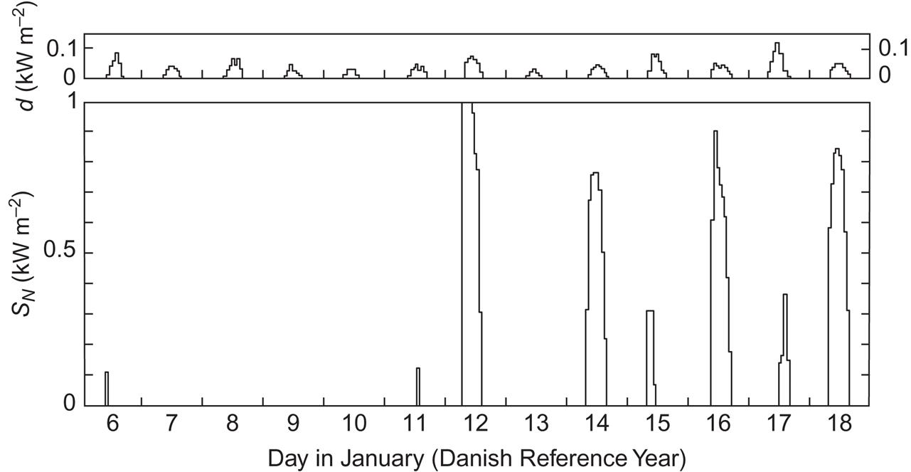
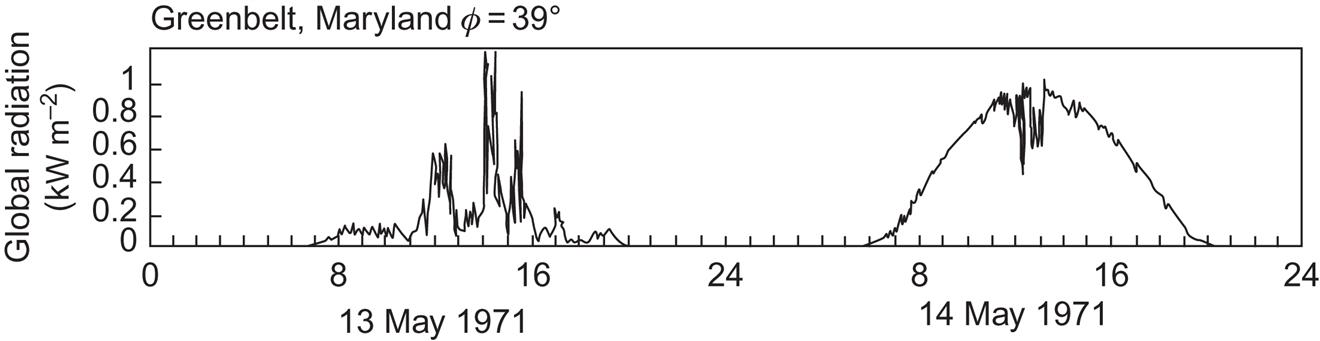
Most of the data presented in sections 3.1.1–3.1.3 are in the form of averages over substantial lengths of time (e.g., a month), although some results are discussed in terms of instantaneous values, such as intensity as a function of solar zenith angle. In order to demonstrate the time structure of radiation quantities more clearly, Fig. 3.20 shows hourly averages of normal incidence radiation, S_N, as well as scattered radiation on a horizontal surface, d, hour by hour over a 13-day period of the Danish reference year (latitude 56°N). For this period in January, several days without any direct (or normal incidence) radiation appear consecutively, and the scattered radiation is quite low. On the other hand, very clear days occasionally occur in winter, as witnessed by the normal flux received on 12 January in Fig. 3.20. Fluctuations within each hour are also present, as can be seen from the example shown in Fig. 3.21. The data are for two consecutive days at a latitude of about 39°N (Goddard Space Flight Center in Maryland; Thekaekara, 1976), collected at 4-s intervals. The figure conveys the picture of intense fluctuations, particularly on a partially cloudy day.

Figure 3.20 Hourly values of the normal incidence flux, S_N, and the scattered flux, d, on a horizontal plane for the Danish reference year, ϕ=56°N. Thirteen consecutive winter days are shown.

Figure 3.21 Two days of continuous recording of total short-wavelength flux on a horizontal plane. Based on Thekaekara (1976).

3.1.5.1 Geographical distribution of solar power

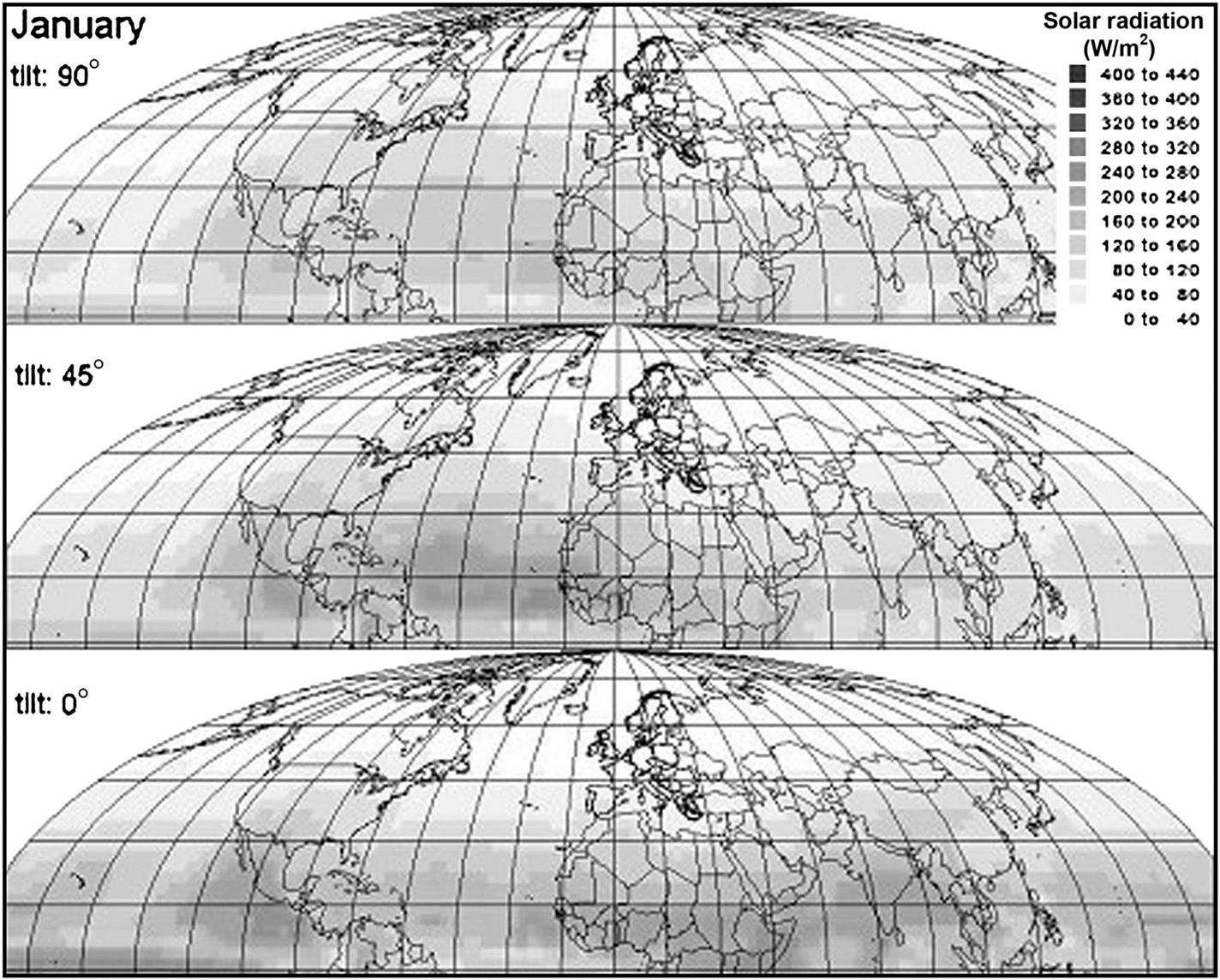
The geographical distribution of average incoming (short-wave) solar radiation on a horizontal plane is shown in Fig. 3.1a–d for each of the four seasons. The data exhibit considerable dependence on conditions of cloud cover and other variables influencing the disposition of radiation on its way from the top to the bottom of the atmosphere. These data form the basis for further analysis in terms of suitability of the power flux for energy conversion in thermal and electricity-producing devices (Chapter 4). Methods for estimating solar radiation on inclined surfaces from the horizontal data are introduced in Chapter 6, along with an appraisal of the fraction of the solar resource that may be considered of practical use after consideration of environmental and area use constraints.

3.1.5.2 Power duration curves

The accumulated frequency distribution is called a power duration curve, since it gives the fraction of time during which the energy flux exceeds a given value E, as a function of E. Figure 3.22a gives power duration curves for total and direct radiation on a horizontal surface and two southward inclined surfaces for a location at latitude ϕ=56°N (Danish reference year, cf. European Commission, 1985). Since data for an entire year have been used, it is not surprising that the energy flux is non-zero for approximately 50% of the time. The largest fluxes, above 800 W m⁻², are obtained for only a few hours a year, with the largest number of hours with high incident flux being for a surface inclined about 45° (cf. Fig. 3.16). The shape of the power duration curve may be used directly to predict the performance of a solar energy device, if this is known to be sensitive only to fluxes above a certain minimum value, say, 300 W m⁻². The power duration curves for direct radiation alone are shown on the right. They are relevant for devices sensitive only to direct radiation, such as most focusing collectors.

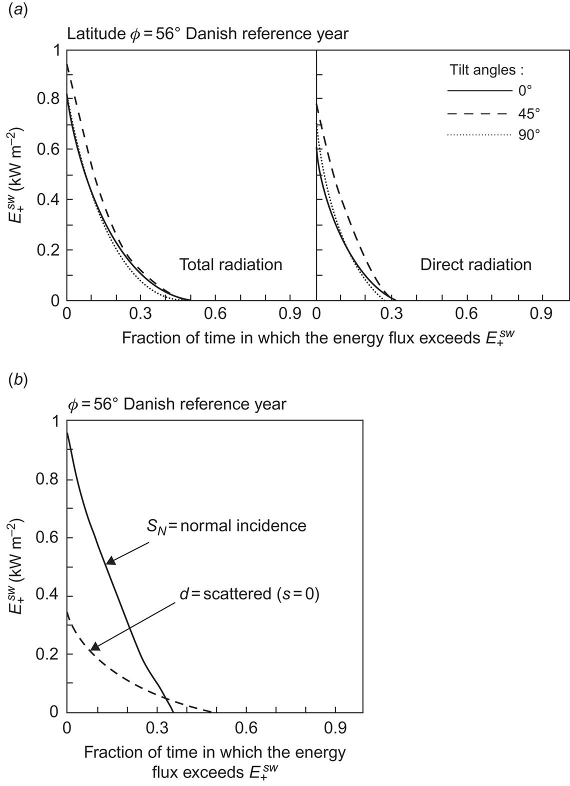
Figure 3.22 (a) One-year power duration curves of total (*left side*) and direct (*right side*) short-wavelength radiation on south-facing surfaces of three different inclinations, based on the Danish reference year, ϕ=56°N. (b) One-year power duration curves of normal incidence radiation alone, and of scattered radiation alone, based on the Danish reference year (ϕ=56°N). The normal incidence curve would correspond to the radiation received by a fully tracking instrument. The curve for scattered radiation is for a horizontal surface.

Figure 3.22b gives the power duration curves for normal incidence radiation, S_N, and for scattered radiation on a horizontal plane, d. The normal incidence curve is of interest for fully tracking devices, that is, devices that are being continuously moved in order to face the direction of the Sun. By comparing Fig. 3.22b with Fig. 3.22a, it can be seen that the normal incidence curve lies substantially above the direct radiation curve for an optimum but fixed inclination (s=45°). The power duration curve for normal incidence radiation is not above the curve for total radiation at s=45°, but it would be if the scattered radiation received by the tracking plane normal to the direction of the Sun were added to the normal incidence (direct by definition) radiation. The power duration curve for scattered radiation alone is also shown in Fig. 3.22b for a horizontal plane. The maximum scattered flux is about 350 W m⁻², much higher than the fluxes received during the winter days shown in Fig. 3.20.

3.2 Wind

It follows from the discussion in section 2.4.1 that the kinetic energy content of the atmosphere, on average, equals about seven days of kinetic energy production or dissipation, also assuming average rates. Utilizing wind energy means installing a device that converts part of the kinetic energy in the atmosphere to, say, useful mechanical energy, i.e., the device draws primarily on the energy stored in the atmospheric circulation and not on the energy flow into the general circulation (1200 TW according to Fig. 2.90). This is also clear from the fact that the production of kinetic energy, i.e., the conversion of available potential energy into kinetic energy, according to the general scheme of Fig. 2.54, does not take place to any appreciable extent near the Earth’s surface. Newell et al. (1969) give height–latitude distributions of the production of zonal kinetic energy for different seasons. According to these distributions, the regions of greatest kinetic energy, the zonal jet-streams at mid-latitudes and a height of about 12 km (see Fig. 2.49), are maintained from conversion of zonal available potential energy in the very same regions.

One of the most important problems to resolve in connection with any future large-scale energy extraction from the surface boundary region of the atmosphere’s wind energy storage is that of the nature of the mechanism for restoring the kinetic energy reservoir in the presence of man-made energy extraction devices. To a substantial extent, this mechanism is known from the study of natural processes by which energy is removed from the kinetic energy storage in a given region of the atmosphere. The store of energy is replenished by the aforementioned conversion processes, by which kinetic energy is formed from the much larger reservoir of available potential energy (four times larger than the kinetic energy reservoir, according to section 2.4.1). The available potential energy is created by temperature and pressure differences, which in turn are formed by the solar radiation flux and the associated heat fluxes.

3.2.1 Wind velocities

3.2.1.1 The horizontal wind profile

The horizontal components of the wind velocity are typically two orders of magnitude larger than the vertical component, but the horizontal components may vary a great deal with height under the influence of frictional and impact forces on the ground (Fig. 2.52) and the geostrophic wind above, which is governed by the Earth’s rotation (see section 2.3.1). A simple model for the variation of horizontal velocity with height in the lower (Prandtl) planetary boundary layer, assuming an adiabatic lapse rate (i.e., temperature gradient, cf. Eq. 2.32) and a flat, homogeneous surface, is given in (2.34).

The zero point of the velocity profile is often left as a parameter, so that (2.34) is replaced by

$u = κ^{- 1} {(τ / ρ)}^{1 / 2} \log ((z + z_{0} - d_{0}) / z_{0})$ $u = κ^{- 1} {(τ / ρ)}^{1 / 2} \log ((z + z_{0} - d_{0}) / z_{0})$ (3.21)

(3.21)

The zero displacement, d₀, allows the zero point of the profile to be determined independently of the roughness length z₀, both being properties of the surface. This is convenient, for example, for woods and cities with roughness lengths from about 0.3 m to several meters, for which the velocity profile “starts” at an elevation (of maybe 10 or 50 m) above the ground. For fixed z₀ and d₀, a family of profiles is described by (3.21), depending only on the parameter (τ/ρ)^1/2, called the friction velocity. For a given location, it is essentially determined by the geostrophic wind speed, still assuming an adiabatic (“neutral”) temperature profile.

If the atmosphere is not neutral, the model leading to (3.21) has to be modified. In fact, (2.34) may be viewed as a special case in a more general theory, due to Monin and Obukhov (1954) (see also Monin and Yaglom, 1965), according to which the wind speed may be expressed as

$u (z) = κ^{- 1} {(τ / r)}^{1 / 2} (f (z / L) - f (z_{0} / L)) .$ $u (z) = κ^{- 1} {(τ / r)}^{1 / 2} (f (z / L) - f (z_{0} / L)) .$

Only in the case of an adiabatic lapse rate is the function f equal to a logarithm. This case is characterized by zL, where the parameter L describing the atmosphere’s degree of stability may be written

$L = c_{p} ρ {(τ / ρ)}^{3 / 2} T_{0} / (g κ Q_{0}) .$ $L = c_{p} ρ {(τ / ρ)}^{3 / 2} T_{0} / (g κ Q_{0}) .$ (3.22)

(3.22)

L is called the Monin–Obukhov length, g is the acceleration of gravity, and T₀ and Q₀ are the temperature and heat flux at the surface. Thus, L is a measure of the transport of heat near the surface, which again determines the stability of the atmosphere. If the heat flux is sufficiently large and directed from ground to atmosphere (Q₀ and thus L negative), then transport of heat and matter is likely to be highly convective and unstable, so that there will be rapid mixing and therefore less variation of wind speed with height. On the other hand, if Q₀ and L are positive, the atmosphere becomes stable, mixing processes become weak, and stratification becomes pronounced, corresponding to almost laminar motion with increasing wind speed upward.

The connection between L and the temperature gradient becomes clear in the convective case, in which one can prove that z/L equals the Richardson number,

$R i = g \frac{1}{θ} \frac{\partial θ}{\partial z} / {(\frac{\partial u}{\partial z})}^{2},$ $R i = g \frac{1}{θ} \frac{\partial θ}{\partial z} / {(\frac{\partial u}{\partial z})}^{2},$ (3.23)

(3.23)

where θ is the potential temperature (2.52). From the definition,

$\frac{\partial θ}{\partial z} = \frac{θ}{T} (\frac{\partial T}{\partial z} - \frac{c_{P} - c_{V}}{c_{P}} \frac{T}{P} \frac{\partial P}{\partial z}),$ $\frac{\partial θ}{\partial z} = \frac{θ}{T} (\frac{\partial T}{\partial z} - \frac{c_{P} - c_{V}}{c_{P}} \frac{T}{P} \frac{\partial P}{\partial z}),$

which according to (2.32) is a direct measure of the deviation from adiabaticity. The adiabatic atmosphere is characterized by Ri=0. The identity of z/L and Ri is easy to derive from (2.29), (2.31), and (2.33), but the linear relationship l=κz (2.33) may not be valid in general. Still, the identity may be maintained, if the potential temperature in (3.6) is regarded as a suitably defined average.

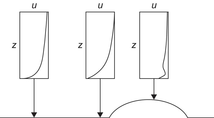
Figure 3.23 gives an example of calculated velocity profiles for neutral, stable, and unstable atmospheres, assuming fixed values of z₀ (0.01 m, a value typical of grass surfaces) and (τ/ρ)^1/2=0.5 m s⁻¹. (Based on Frost, 1975.) Many meteorological stations keep records of stability class, based on either observed turbulence, Ri, or simply ∂T/∂z. Thus, it is often possible with a certain amount of confidence to extrapolate wind speed measurements taken at one height (e.g., the meteorological standard of 10 m) to other heights that are interesting from the point of view of wind energy extraction.

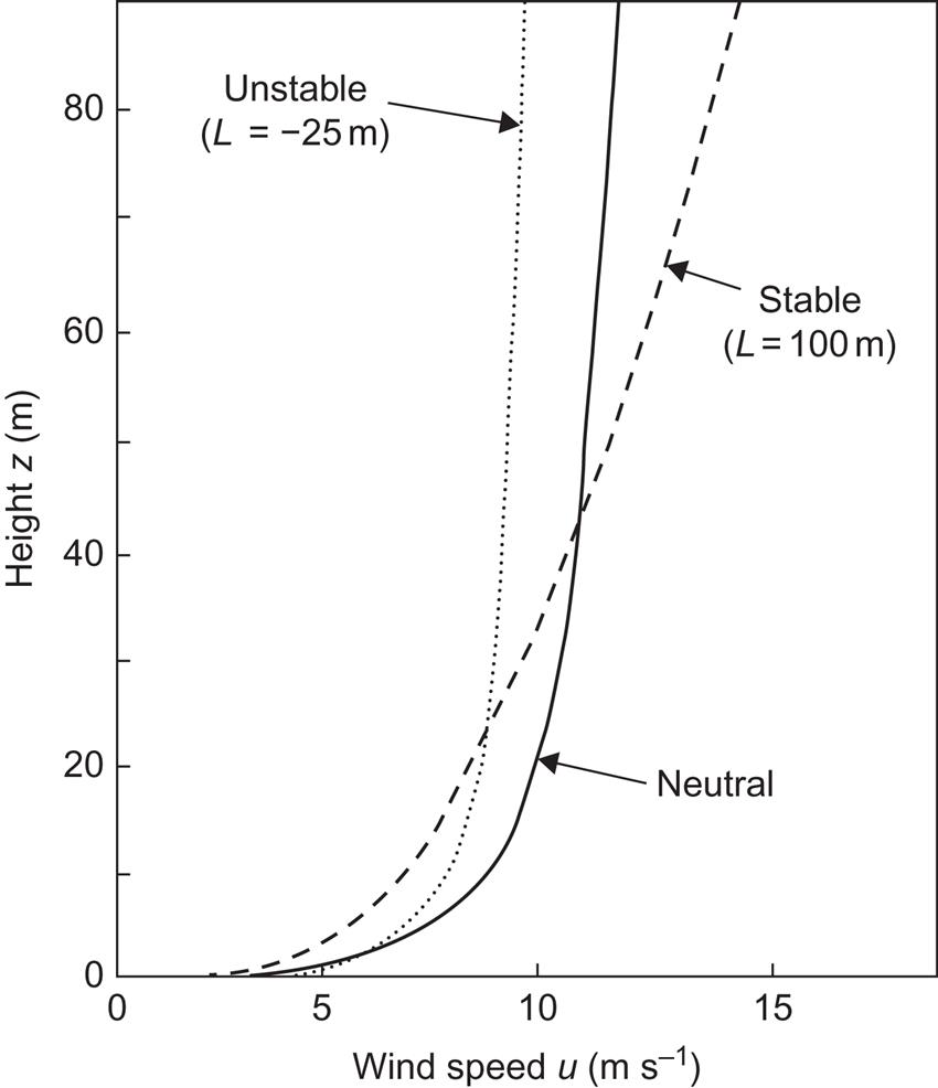
Figure 3.23 Wind speed profiles (i.e., variation with height) for a flat terrain characterized by a roughness length of 0.01 m and for a friction velocity of (τ/ρ)^1/2=0.5 m s⁻¹. The three different curves correspond to an atmosphere that is neutral (has an adiabatic lapse rate), stable, or unstable. The stability is expressed in terms of the Monin–Obukhov length. Based on Frost (1975).

The wind profiles also show that a wind energy conversion device spanning several tens of meters and placed in the planetary boundary layer is likely to experience substantially different wind velocities at different ends of the device (e.g., rotor blades).

The simple parametrizations of wind profiles considered above can be expected to be valid only over flat and homogeneous terrain. The presence of obstacles, such as hills, vegetation of varying height, and building structures, may greatly alter the profiles and will often create regions of strong turbulence, where no simple average velocity distribution will give an adequate description. If an obstacle like a hilltop is sufficiently smooth, however, and the atmospheric lapse rate neutral or stable, the possibility exists of increasing the wind speed in a regular fashion at a given height where an energy collecting device may be placed. An example of this is shown in Fig. 3.24, based on a calculation by Frost et al. (1974). The elliptical hill shape extends infinitely in the direction perpendicular to the plane depicted. However, most natural hill shapes do not make a site more suitable for energy extraction. Another possibility of enhanced wind flow at certain heights exists in connection with certain shapes of valleys, which may act like a shroud to concentrate the intensity of the wind field, while still preserving its laminar features (see, for example, Frost, 1975). Again, if the shape of the valley is not perfect, regions of strong turbulence may be created and the suitability for energy extraction diminishes.

Figure 3.24 Wind speed profiles for a wind directed perpendicular to an elliptically shaped hill for two locations upwind, plus at the top of the hill. The profile far away from the disturbance corresponds to a surface of roughness length 0.005 m, a friction velocity of 0.4 m s⁻¹, and a neutral atmosphere. Based on Frost *et al*. (1974).

Only in relatively few cases can the local topography be used to enhance the kinetic energy of the wind at heights suitable for extraction. In the majority of cases, the optimum site selection will be one of flat terrain and smoothest possible surface in the directions of the prevailing winds. Since the roughness length over water is typically of the order 10⁻³ m, the best sites for wind energy conversion will usually be coastal sites with large fetch regions over water.

3.2.1.2 Wind speed data

Average wind speeds give only a very rough idea of the power in the wind (which is proportional to u³) or the kinetic energy in the wind (which is proportional to u²), owing to the fluctuating part of the velocity, which makes the average of the cube of u different from the cube of the average, etc. Whether the extra power of the positive speed excursions can be made useful depends on the response of the particular energy conversion device to such fluctuations.

For many locations, only average wind speed data are available, and since it is usually true in a qualitative way that the power that can be extracted increases with increasing average wind speed, a few features of average wind speed behavior are described.

In comparing wind speed data for different sites, the general wind speed–height relation (such as the ones shown in Fig. 3.23) should be kept in mind, along with the fact that roughness length, average friction velocity, and statistics of the occurrence of different stability classes are also site-dependent quantities.

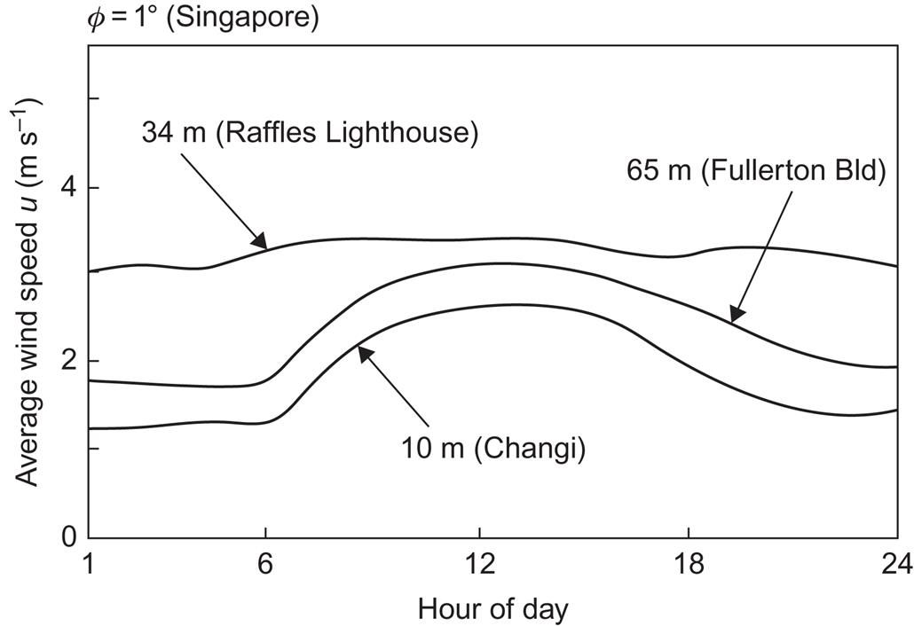
Figure 3.25 shows the seasonal variation of wind speed, based on monthly average values, for selected locations. Except for Risø (Denmark) and Toronto, the sites represent near optimum wind conditions for their respective regions. Not all parts of the Earth are as favored with winds as the ones in Fig. 3.25. Figure 3.26 shows the variation of average wind speed throughout the day at two shoreline sites and one maritime site in Singapore. The average wind speed at the latter site is slightly over 3 m s⁻¹, and there is little seasonal variation. At the two land-based observational stations, the average speed is only around 2 m s⁻¹, with very little gain if the height is increased from 10 to 65 m.

Figure 3.25 Seasonal variation of average wind speed for selected locations and heights. Torsminde data for 1961 from Jensen (1962), Givat Hamore data Nov. 1959 to Oct. 1960 from Frenkiel (1964), Risø 1958–1967 data from Petersen (1974), Toronto 1955–1972 data from Brown and Warne (1975), St. Paul Island 1943–1971 data from Wentink (1976), and the Ludington 1970, 1972 data from Asmussen (1975).

Figure 3.26 Variations of average wind speed with hour of the day for three Singapore stations. The data cover the period 1970–1974. Based on Nathan *et al*. (1976).

Global wind speed data are shown in Figs. 2.83–2.84. Figures 3.27 and 3.28 show the levels of power in the wind at potential hub height for wind turbines (about 70 m), on a seasonal base, using data from NCEP-NCAR (1998). These data have been made more consistent by a re-analysis method (Kalnay et al., 1996), in which general circulation models have been run to improve predictions in areas of little or poor data. The construction of power in the wind estimates from wind speed data is explained in section 6.3.1. It involves an averaging of circulation model data from height levels of 1000 and 925 mb (expressed as pressure levels), plus an empirical way of relating the average of the third power of the wind speed (the power) to the third power of the average wind speed. This procedure necessarily yields very approximate results. The main observation is that the highest power levels are found over oceans, including some regions close to shorelines. This points to the possibility of obtaining viable extraction of wind power from offshore plants located at suitable shallow depths. It is also seen that seasonal variations are significant, particularly over large continents. A new, more accurate method of determining offshore potential wind power production is presented in section 6.3.1.

Figure 3.27 (a,b) Maps of wind power regimes for January and April 1997, based on NCEP-NCAR (1998). The power levels are estimated for a height of 70 m above ground, presently a typical hub height for wind turbines. The method of estimation is explained in section 6.3.1. [These and following area-based geographical information system (GIS) maps are from Sørensen and Meibom (1998), copyright B. Sørensen.].

Figure 3.28 (a,b) Maps of wind power regimes for July and October 1997, based on NCEP-NCAR (1998). The power levels are estimated for a height of 70 m above ground, presently a typical hub height for wind turbines. The method of estimation is explained in section 6.3.1.

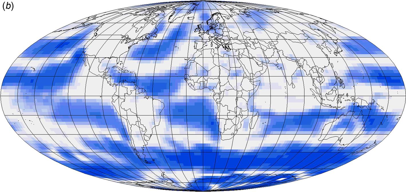
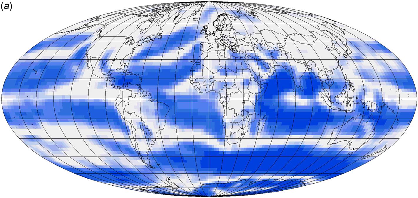
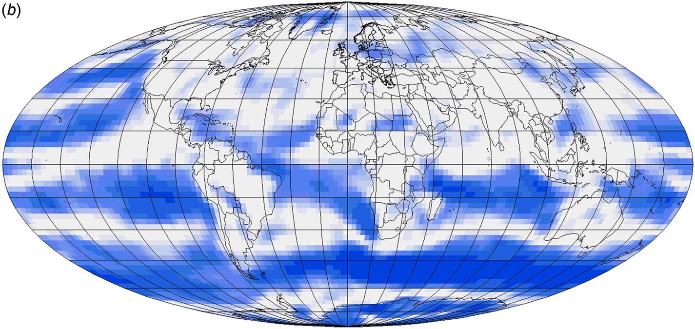
Figure 3.29 shows an example of measured wind profiles as a function of the hour of the day, averaged over a summer and a winter month. The tendency to instability due to turbulent heat transfer is seen during summer day hours (cf. the discussion above). Changes in wind direction with height have been measured (e.g., by Petersen, 1974). In the upper part of the planetary boundary layer, this is simply the Ekman spiral (cf. section 2.3.2).

Figure 3.29 Variation of wind speed height profile with the hour of day at Risø, Denmark (56°N). Each curve has been averaged over all data from the period 1958–1967 for one winter or summer month. Based on data from Petersen (1974).

The continuation of the velocity profile above the Prandtl boundary layer may be important in connection with studies of the mechanisms of restoring kinetic energy lost to an energy extraction device (e.g., investigations of optimum spacing between individual devices). Extraction of energy in the upper troposphere does not appear attractive at the present technological level, but the possibility cannot be excluded. Figure 3.30 shows the 10-year average wind profile at Risø (ϕ=56°) matched to a profile stretching into the stratosphere, based on German measurements. The average wind speed near the tropopause compares well with the zonal means indicated in Fig. 2.49.

Figure 3.30 Annual average wind speed vs. height profile at latitudes 50–56°N. The lower part of the curve is based on Risø data (Petersen, 1974), and the upper part is based on a set of curves derived from German measurements (Hütter, 1976). The one matching the lower part of the curve has been selected. Also indicated (*dashed line*) is an average height profile of the air density, used in the construction of Figs. 3.31–3.33.

3.2.1.3 Height scaling and approximate frequency distribution of wind

In practical applications, some approximate relations are often employed in simple wind power estimates. One describes the scaling of wind speeds with height, used, for example, to estimate speed u at a wind turbine hub height z from measured data at another height z₁. It is based on (3.21):

$u (z) = u (z_{1}) \log ((z - z_{1}) / z_{0}),$ $u (z) = u (z_{1}) \log ((z - z_{1}) / z_{0}),$ (3.24)

(3.24)

where the parameter z₀ describes the local roughness of the surface. However, (3.24) is valid only for stable atmospheres. Another often-used approximation is the Weibull distribution of wind speeds v over time at a given location (f is the fraction of time in a given speed interval; Sørensen, 1986):

$f (v) = (k / c) {(v / c)}^{k - 1} \exp - {(v / c)}^{k},$ $f (v) = (k / c) {(v / c)}^{k - 1} \exp - {(v / c)}^{k},$ (3.25)

(3.25)

where the parameter k is around 2 and c around 8, both with considerable variations from site to site.

3.2.2 Kinetic energy in the wind

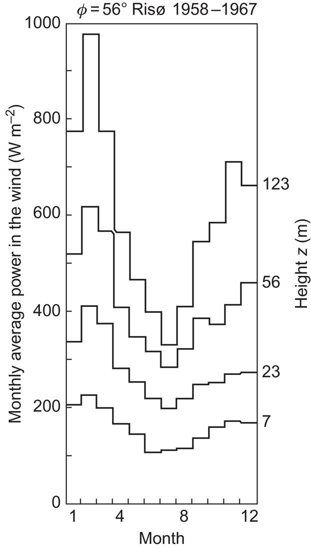
In analogy to Fig. 3.30, the height variation of the kinetic energy density is obtained in the form shown in Fig. 3.31. The density variation used in (2.55) is the one indicated in Fig. 3.30, and the hourly data from Risø, Denmark, have been used to construct the kinetic energy at heights of 7–123 m, the average values of which form the lower part of the curve in Fig. 3.31. The fluctuations in wind speed diminish with height (cf. Fig. 3.36), and at z=123 m the difference between the annual average of u² and the square of the average u is only about 1%. For this reason, the average wind speeds of Fig. 3.30 were used directly to form the average kinetic energy densities for the upper part of the figure. The kinetic energy density peaks some 3 km below the peak wind speed, owing to the diminishing air density. Fig. 3.31b illustrates, on a non-logarithmic scale, the bend of the curve at a height of 1–2 km, where the near-logarithmic increase of wind speed with height is replaced by a much stronger increase.

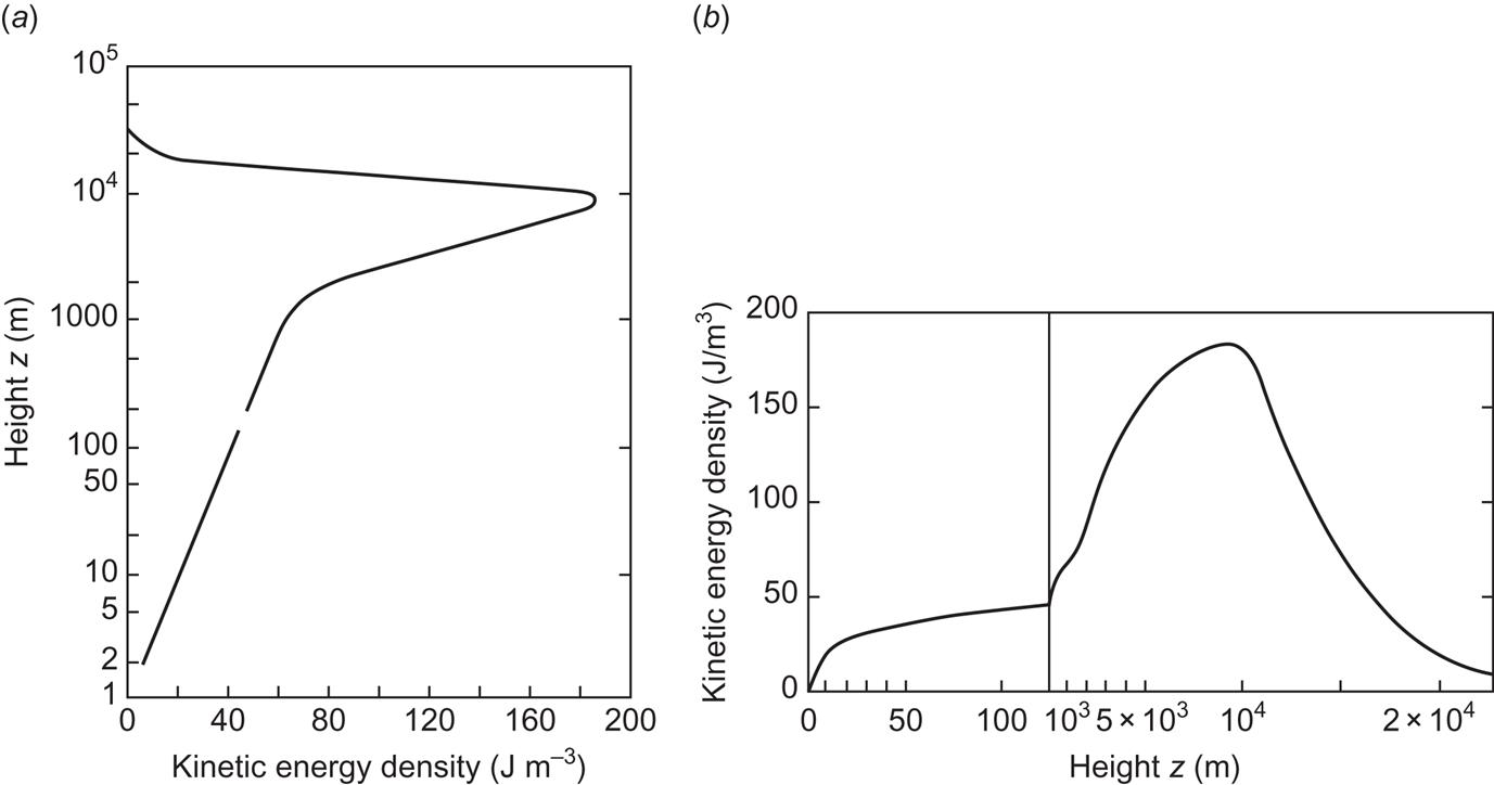
Figure 3.31 (a,b) Annual average height profile of kinetic energy density at latitudes 50°–56°N. At low height, the curve is based on hourly data from Risø (Petersen, 1974), at larger heights calculated from the wind speeds of Fig. 3.30, neglecting any fluctuations. Fig. 3.31b is the same on two linear-scale segments.

The kinetic energy density curve of Fig. 3.31 may readily be integrated to give the accumulated amount of kinetic energy below a given height, as shown in Fig. 3.32. This curve illustrates the advantage of extending the sampling area of a wind energy-collecting device into the higher regions of the atmosphere. The asymptotic limit of the accumulation curve is close to 2×10⁶ J m⁻² of vertical column. This order of magnitude corresponds to that of the estimate given in Fig. 2.54, of 8×10⁵ J m⁻² as a global average of zonal kinetic energy, plus a similar amount of eddy kinetic energy. The eddy kinetic energy, which is primarily that of large-scale eddies (any deviation from zonal means), may, in part, be included in the curve based on Fig. 3.29, which gives mean wind speed and not zonal mean. Since the data are for latitude 50°N–56°N, it may also be assumed that the kinetic energy is above the global average, judging from the latitude distribution of zonal winds given in Fig. 2.49.

Figure 3.32 Accumulated kinetic energy below a given height, for latitudes around 50°–56°N, obtained by integration of the curve in Fig. 3.31.

3.2.3 Power in the wind

The energy flux passing through an arbitrarily oriented surface exposed to the wind is obtained by multiplying the kinetic energy density by v·n, where v is the wind velocity and n is the normal to the surface. The energy flux (power) may then be written

$E = 1 / 2 ρ u^{3} \cos θ,$ $E = 1 / 2 ρ u^{3} \cos θ,$ (3.26a)

(3.26a)

where θ is the angle between v and n. If the vertical component of the wind velocity can be neglected, as well as the short-term fluctuations [termed v′ according to (2.23)], then the flux through a vertical plane perpendicular to the direction of the wind becomes

$E = 1 / 2 \bar{ρ} - {(V *)}^{3},$ $E = 1 / 2 \bar{ρ} - {(V *)}^{3},$ (3.26b)

(3.26b)

where V* is the average, horizontal wind velocity corresponding to a given time-averaging interval (2.21). If the wind speed or direction cannot be regarded as constant over the time interval under consideration, then an average flux (average power) may be defined by

$E = \frac{1}{Δ t} \int_{t_{1}}^{t_{1} + Δ t} \frac{1}{2} ρ v^{3} \cos θ d t_{2},$ $E = \frac{1}{Δ t} \int_{t_{1}}^{t_{1} + Δ t} \frac{1}{2} ρ v^{3} \cos θ d t_{2},$

where both v and θ (and in principle ρ) may depend on the time integrand t₂. A situation often met in practice is one of an energy-collecting device, which is able to follow some of the changes in wind direction, but not the very rapid ones. Such a “yaw” mechanism can be built into the prescription for defining θ, including the effect of a finite response time (i.e., so that the energy-collecting surface is being moved toward the direction the wind had slightly earlier).

Most wind data are available in a form where short-term variations have been smoothed out. For example, the Risø data used in the lower part of Fig. 3.30 are 10-min averages centered on every hour. If such data are used to construct figures for the power in the wind, as in Figs. 3.33–3.34 and the duration curves in Figs. 3.39–3.40, then two sources of error are introduced. One is that random excursions away from the average wind speed will imply a level of power that on average is larger than that obtained from the average wind speed [owing to the cubic dependence in (3.24)]. The other is that, owing to changes in wind direction, the flux calculated from the average wind speed will not be passing through the same surface during the entire averaging period, but rather through surfaces of varying orientation. This second effect will tend to make the predicted power level an overestimate for any surface of fixed orientation.

Figure 3.33 Annual average height profile of power in the wind, at latitudes 50°–56°N. The lower part of the curve has been calculated from the Risø data of Petersen (1974), and the upper part is from the wind speeds of Fig. 3.30, neglecting any fluctuations.

Figure 3.34 Monthly average power in the wind at Risø, Denmark, for different heights. Calculation based on 10 years of data (Petersen, 1974).

Jensen (1962) overcame both of these difficulties by basing his measurements of power in the wind on a statistical ensemble of instantaneous measurements and by mounting unidirectional sensors on a yawing device that was chosen to respond to changing wind directions in a manner similar to that of the wind energy generators being considered. However, it is not believed that monthly average power or power duration curves will be substantially affected by using average data like those from Risø (note that the ergodic hypothesis in section 2.3.3, relating the time averages to the statistical ensemble means, is not necessarily valid if the time averages are formed only over one 10-min interval for each hour).

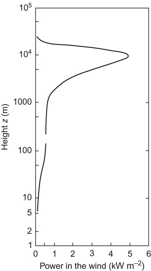
In the upper part of Fig. 3.33, the power has been calculated from the average wind speeds of Fig. 3.30, using (3.25). The seasonal variations at lower heights are shown in Fig. 3.34. It is clear that the amount of seasonal variation increases with height. This indicates that the upper part of Fig. 3.33 may well underestimate the average of summer and winter energy fluxes.

Additional discussion of the power in the wind, at different geographical locations, is found below in section 3.2.4. The overall global distribution of power in the wind at different seasons is shown in Fig. 3.27.

3.2.4 Variability in wind power

An example of short-term variations in wind speed at low height is given in Fig. 3.35. These fluctuations correspond to the region of frequencies above the spectral gap of Fig. 2.109. The occurrences of wind “gusts,” during which the wind speed may double or drop to half the original value over a fraction of a second, are clearly of importance for the design of wind energy converters. On the other hand, the comparison made in Fig. 3.35 between two simultaneous measurements at distances separated horizontally by 90 m shows that little spatial correlation is present between the short-term fluctuations. Such fluctuations would thus be smoothed out by a wind energy conversion system, which comprises an array of separate units dispersed over a sufficiently large area.

Figure 3.35 Short-term variation in wind speed, from simultaneous records at two locations 90 m apart (measuring height probably in the range of 5–10 m). Based on Banas and Sullivan (1976).

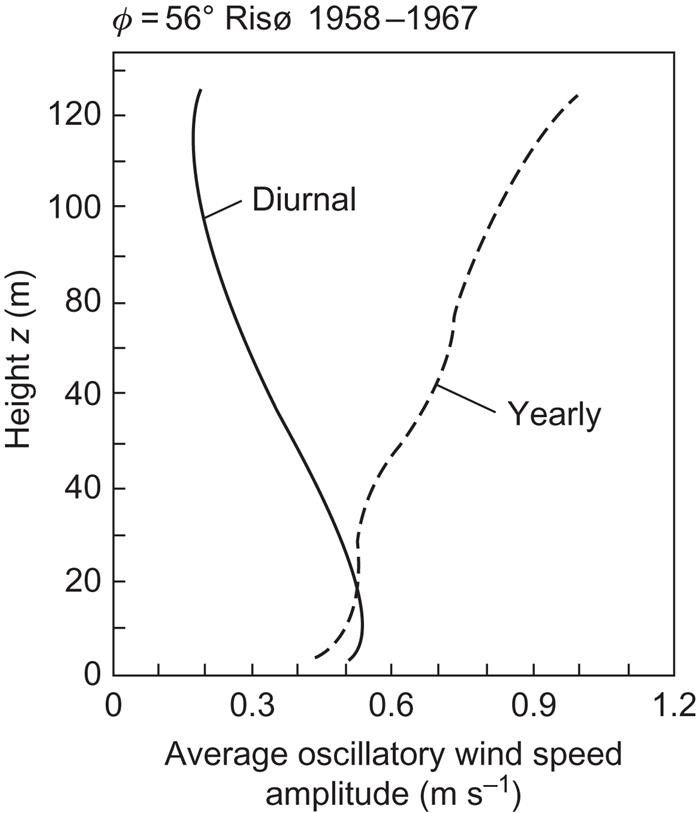
The trends in amplitudes of diurnal and yearly wind speed variations are displayed in Fig. 3.36, as functions of height (Petersen, 1974). Such amplitudes are generally site-dependent, as one can deduce, for example, from Figs. 3.26 and 3.28 for diurnal variations and from Fig. 3.25 for seasonal variations. The diurnal amplitude in Fig. 3.26 diminishes with height, while the yearly amplitude increases with height. This is probably a general phenomenon when the wind approaches its geostrophic level, but the altitude dependence may depend on geographical position and local topography. At some locations, the diurnal cycle shows up as a 24-h peak in a Fourier decomposition of the wind speed data. This is the case at Risø, Denmark, as seen from Fig. 3.37, while the peak is much weaker at the lower height used in Fig. 2.109. The growth in seasonal amplitude with height is presumably determined by processes taking place at greater height (cf. Figs. 2.49 and 2.50) as well as by seasonal variations in atmospheric stability, etc.

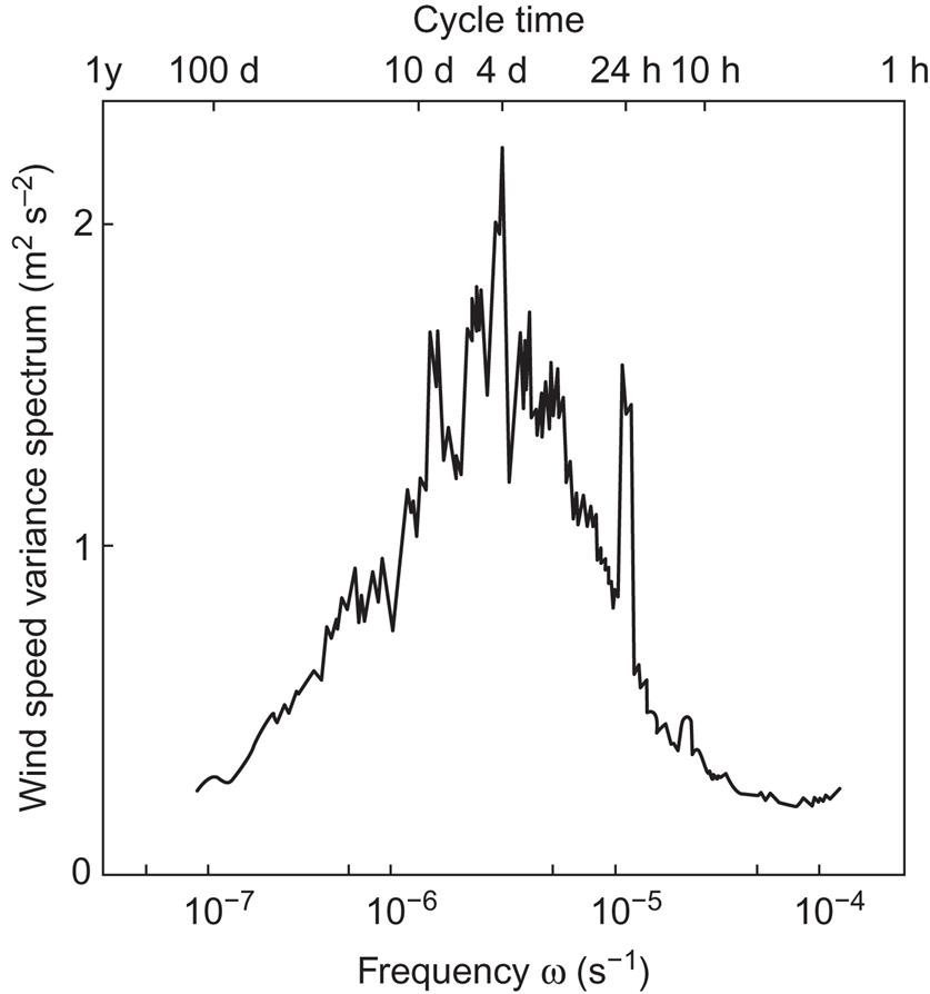
Figure 3.36 Height dependence of diurnal and yearly amplitude of oscillation of the wind speed at Risø. The average estimate is based on a Fourier decomposition of the data with no smoothing (Petersen, 1974).

Figure 3.37 Variance spectrum of horizontal wind speeds at Risø (ϕ=56°N) at a height of 56 m (based on 10 years of observation; Petersen, 1974). The spectrum is smoothed by using frequency intervals of finite length (cf. Fig. 2.109 of section 2.5.2, where similar data for a height of 7 m are given).

The wind speed variance spectrum (defined in section 2.5.2 in connection with Fig. 2.109) shown in Fig. 2.42 covers a frequency interval between the yearly period and the spectral gap. In addition to the 24-h periodicity, the amplitude of which diminishes with increasing height, the figure exhibits a group of spectral peaks with periods in the range 3–10 days. At the selected height of 56 m, the 4-day peak is the most pronounced, but moving up to 123 m, the peak period around 8 days is more marked (Petersen, 1974). It is likely that these peaks correspond to the passage time of typical meso-scale front and pressure systems.

In analyzing the variability of wind speed and power during a certain period (e.g., month or a year), the measured data are conveniently arranged in the forms of frequency distributions and power duration curves, much in the same manner as discussed in section 3.1.5. Figure 3.38 gives the 1-year frequency distribution of wind speeds at two Danish locations for a height of about 50 m. The wind speed frequency distribution (dashed curve) at Gedser (near the Baltic Sea) has two maxima, probably associated with winds from the sea and winds approaching from the land (of greater roughness). However, the corresponding frequency distribution of power (top curve) does not exhibit the lower peak, as a result of the cubic dependence on wind speed. At the Risø site, only one pronounced maximum is present in the wind speed distribution. Several irregularities in the power distribution (which are not preserved from year to year) bear witness to irregular landscapes with different roughness lengths, in different directions from the meteorological tower.

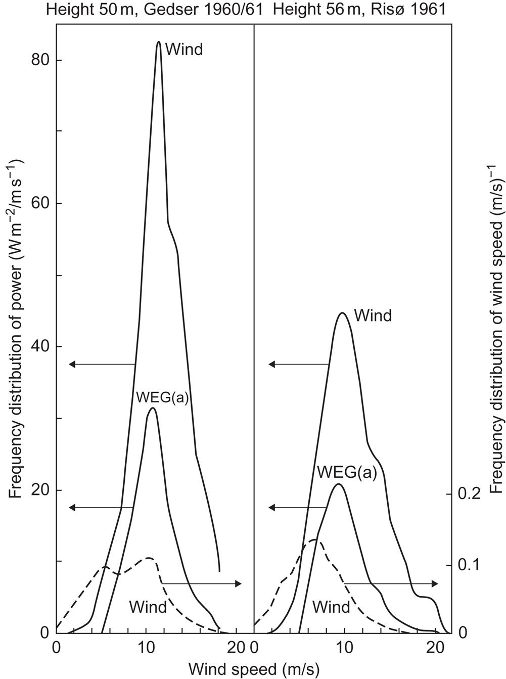
Figure 3.38 Frequency distribution of wind speed (*right-hand scale*) and of power for a height of about 50 m at two Danish sites. The middle curves give frequency distributions for the output of a typical wind energy generator (Sørensen, 1978).

Despite the quite different appearance of the wind speed frequency distribution, the power distribution for the two Danish sites peaks at roughly the same wind speed, between 10 and 11 m s⁻¹.

3.2.4.1 Power duration curves

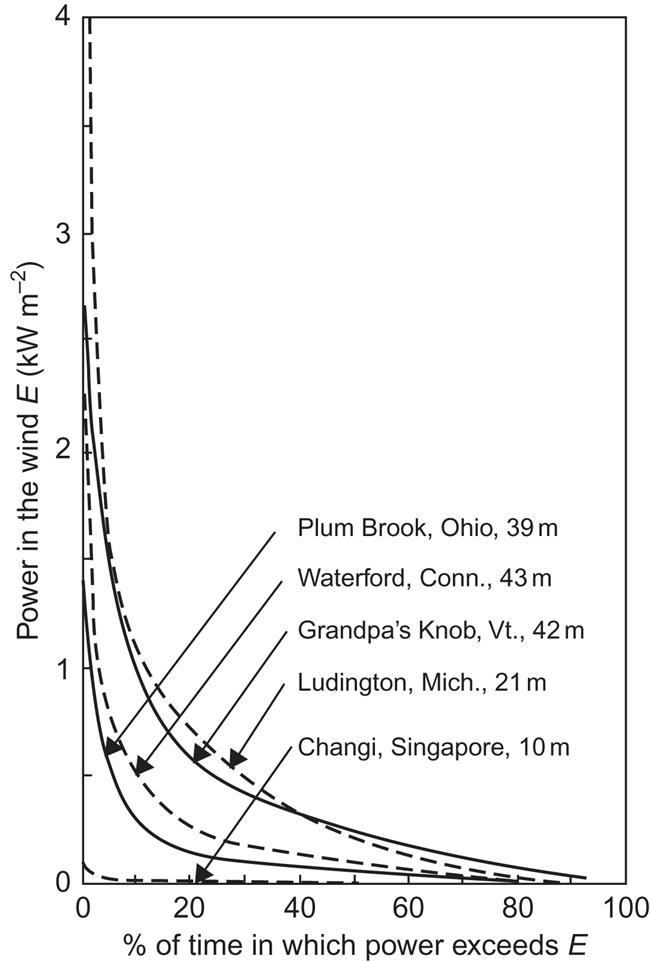
On the basis of the frequency distributions of the wind speeds (or alternatively that of power in the wind), power duration curves can be constructed giving the percentage of time when the power exceeds a given value. Figures 3.39 and 3.40 give a number of such curves, based on periods of a year or more. In Fig. 3.39, power duration curves are given for four U.S. sites that have been used or are being considered for wind energy conversion and for one of the very-low-wind Singapore sites.

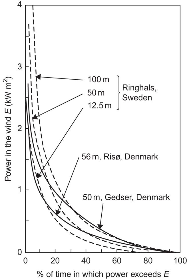
Figure 3.39 One-year duration curves of power in the wind, for a number of locations and heights [Swanson *et al*., 1975 (Plum Brook and Grandpa’s Knob); Coste, 1976 (Waterford); Asmussen, 1975 (Ludington); Nathan *et al*., 1976 (Changi)].

Figure 3.40 One-year duration curves of power in the wind at Scandinavian sites (including different heights at the Ringhals site). Based on data from Ljungström (1975) (Ringhals); Petersen (1974) (Risø); Jensen (1962) (Gedser).

In Fig. 3.40, power duration curves are given for the two different Danish sites considered in Fig. 3.38, as well as for a site on the west coast of Sweden, at three different heights. The three curves for the same site have a similar shape, but in general the shape of the power duration curves in Figs. 3.39 and 3.40 depends on location. Although the Swedish Ringhals curves have non-negligible time percentages with very large power, the Danish Gedser site has the advantage of a greater frequency of medium power levels. This is not independent of conversion efficiency, which typically has a maximum as function of wind speed.

3.3 Water flows and reservoirs, waves, and tides

3.3.1 Ocean currents

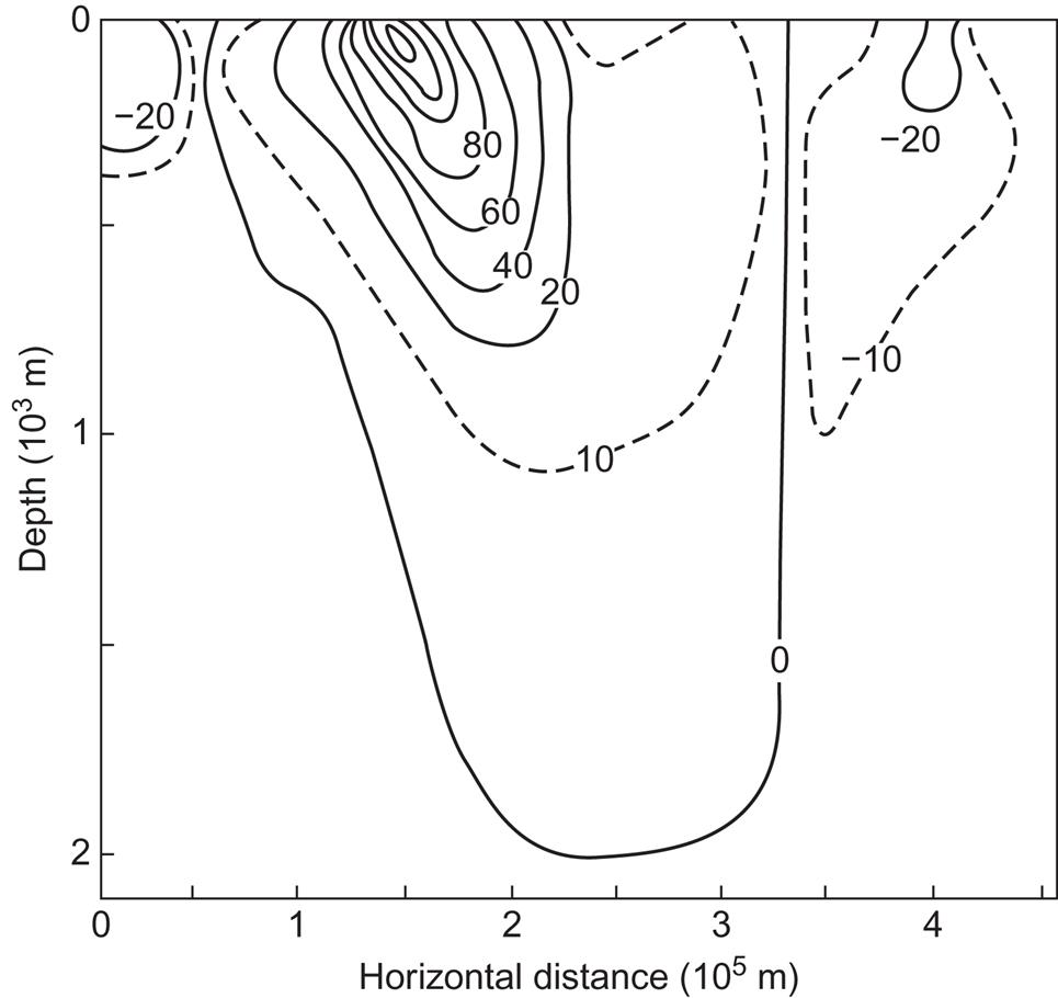
The maximum speed in the center of the Gulf Stream is about 2 m s⁻¹, corresponding to an energy density 1/2ρ_wV_w²=2 kJ m⁻³ and a power of 1/2ρ_wV_w³=4 kW m⁻². This power level, for example, approaches that of wave power at reasonably good sites, taken as power per meter of wave crest rather than per square meter perpendicular to the flow, as used in the above case. However, high average speed of currents combined with stable direction is found only in a few places. Figure 3.41 shows the isotachs in a cross-section of the Gulf Stream, derived from a single set of measurements (in June 1938; Neumann, 1956). The maximum current speed is found at a depth of 100–200 m, some 300 km from the coast. The isotachs expand and become less regular further north, when the Gulf Stream moves further away from the coast (Niiler, 1977).

Figure 3.41 Contours of equal speed (in 10⁻² m s⁻¹) along a cross-section through the Gulf Stream from Bermuda to the U.S. coast. The measurements were performed over a limited period of time (in June 1938, by Neumann, 1956), but they are consistent with other measurements in the same region (e.g., Florida Strait measurements by Brooks and Niiler, 1977).

Even for a strong current like the Gulf Stream, the compass direction at the surface has its most frequent value only slightly over 50% of the time (Royal Dutch Meteorological Institute, as quoted by Neumann and Pierson, 1966), and the power will, on average, deviate from that evaluated on the basis of average current speeds (as is the case for wind or waves) owing to the inequality of <V³> and <V>³.

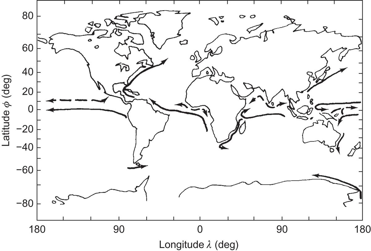
The geographical distribution of the strongest surface currents is indicated in Fig. 3.42. The surface currents in the Atlantic Ocean, along with the horizontal currents at three different depths, are sketched in Fig. 3.43. The current speeds indicated are generally decreasing downward, and the preferred directions are not the same at different depths. The apparent “collision” of oppositely directed currents, e.g., along the continental shelf of Central America at a depth of around 4 km, conceals the vertical motion that takes place in most of these cases. Figure 3.44 gives a vertical cross-section with outlined current directions. The Figure shows how the oppositely directed water masses “slide” above and below each other. The coldest water is flowing along the bottom, while the warmer water from the North Atlantic is sliding above the cold water from the Antarctic.

Figure 3.42 Indication of the location of strong surface currents (approximately defined as having average speeds above 0.5 m s⁻¹). Currents drawn with *dashed lines* are characterized by seasonal changes in direction. Based on Defant (1961).

Figure 3.43 Indication of average horizontal current speeds (in 10⁻² m s⁻¹) in the Atlantic Ocean for different depths. Based on Defant (1961).

Figure 3.44 Indication of average current directions within a vertical cross-section of the Atlantic Ocean. Based on Neumann and Pierson (1966).

3.3.1.1 Variability in current power

Although the general features of circulation in the open ocean are described in section 2.3.2, the particular topography of coastal regions may have an important influence on currents. As an example, water forced through a narrow strait may acquire substantial speeds. The strait Storebælt (“Great Belt”) between two Danish isles, which provides an outlet from the Baltic Sea, may serve as an illustration. It is not extremely narrow (roughly 20 km at the measurement site), but narrow enough to exhibit only two current directions, separated by 180°. The currents may seem fairly steady, except for periods when the direction is changing between north-going and south-going velocities, but when the energy flux is calculated from the third powers of the current speeds, the fluctuations turn out to be substantial. Figure 3.45, which gives the power at 3-hour intervals during two weeks of January 1972 clearly illustrates this.

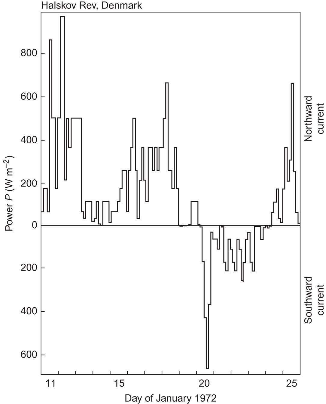
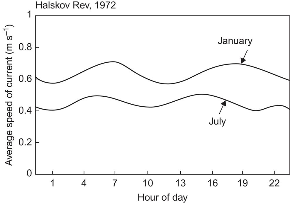
Figure 3.45 Power of surface current, based on observations made at 3-h intervals, for Halskov Rev, Denmark, during a 15-day period in 1972 (the strait is narrow enough to exhibit only two opposite current directions). Based on Danish Meteorological Institute (1973).

Figure 3.46 shows, again for the Halskov Rev position in Storebælt, the variation in current speed with the hour of the day, based on 1-month averages. A 12-hour periodicity may be discerned, at least during January. This period is smaller than the one likely to be found in the open sea due to the motion of water particles in stationary circles under the influence of the Coriolis force [see (2.62)], having a period equal to 12 h divided by sin ϕ (ϕ is the latitude).

Figure 3.46 Dependence of average current speed on the hour of the day, for a summer and a winter month, for Halskov Rev, Denmark. Based on Danish Meteorological Institute (1973).

In Fig. 3.47, the frequency distributions of current speed and power are shown for a summer and a winter month. These curves are useful in estimating the performance of an energy extraction device, and they can be used, for example, to construct the power duration curve of the current motion, as shown in Fig. 3.48. This is the power duration curve of the currents themselves. That of an energy-extracting device will have to be folded with the efficiency function of the device.

Figure 3.47 Frequency distributions of current speeds and power, based on a summer and a winter month (*solid* and *dashed curves*, respectively), for Halskov Rev, Denmark. The data (taken from Danish Meteorological Institute, 1973) have been smoothed in calculating the distributions. The monthly average speed and power are indicated on the figure (in parentheses).

Figure 3.48 Power duration curves for power in currents at Halskov Rev, Denmark, based on a summer and a winter month of 1972. *Thin*, *dashed lines* indicate the monthly average power and the percentage of time during which it is available.

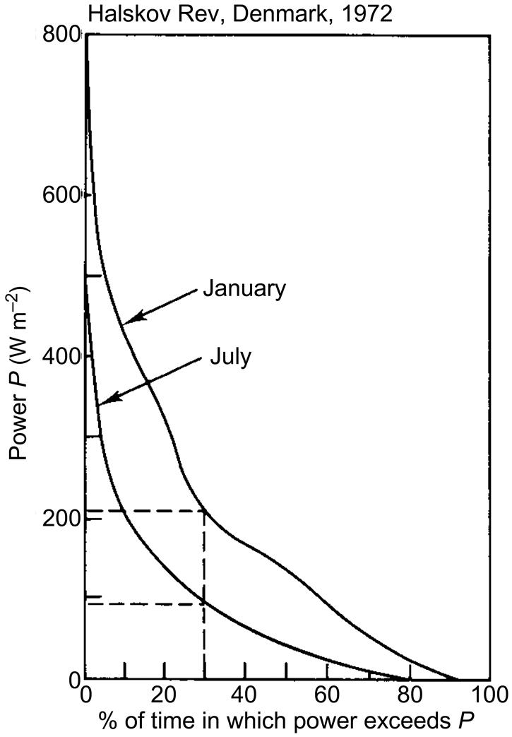
The peak in the frequency distribution of power is at a lower current speed for July than for January, and the average power is 93 W m⁻² in July, as compared with 207 W m⁻² in January (the corresponding kinetic energy densities are 138 and 247 J m⁻³). This indicates that the fluctuations around the average values have a substantial effect on the energy and, in particular, on the power, because from the average current speeds, 0.46 m s⁻¹ (July) and 0.65 m s⁻¹ (January), the calculated kinetic energy densities would have been 108 and 211 J m⁻³, and the power would have taken the values 50 and 134 W m⁻².

Few locations, whether in coastal regions or in open oceans, have higher average current speeds than the Danish location considered in Figs. 3.45–3.48, so that average power levels in the range 100–200 W m⁻² are likely to be more representative than the 4000 W m⁻² found (at least at the time of the measurement reported in Fig. 3.41) in the core of the Gulf Stream. This means that at many locations the power in currents is no greater than that found in the wind at quite low heights (cf. Fig. 3.34). Also, the seasonal variations and fluctuations are similar, which is not unexpected for wind-driven currents. For the currents at greater depths this may not hold true, partly because of the smoothing due to a long turnover time and partly because not all the deep-sea motion is wind driven, but may also be associated with temperature and salinity gradients, as discussed in section 2.3.2.

The power duration curves in Fig. 3.48 may be compared to those of wind power shown in Figs. 3.39 and 3.40. The fraction of time in which the monthly average power is available in the Halskov Rev surface current is 0.3 in both January and July. The overall average power of about 150 W m⁻² is available for about 45% of the time in January, but only 17% of the time in July.

3.3.2 River flows, hydropower, and elevated water storage

The kinetic energy of water flowing in rivers or other streams constitutes an energy source very similar to that of ocean currents. However, rather than being primarily wind driven or caused by differences in the state of the water masses themselves, the river flows are part of the hydrological cycle depicted in Fig. 2.65. Water vapor evaporated into the atmosphere is transported and eventually condensed. It reaches the ground as water or ice, at the elevation of the particular location. Thus, the primary form of energy is potential. In the case of ice and snow, a melting process (using solar energy) is usually necessary before the potential energy of elevation can start to transform into kinetic energy. The origin of many streams and rivers is precisely the ice-melting process, although their flows are joined by ground water flows along their subsequent routes. The area from which a given river derives its input of surface run-off, melt-off, and ground water is called its drainage basin.

The flow of water in a river may be regulated by means of dam building, if suitable reservoirs exist or can be formed. In this way, the potential energy of water stored at an elevation can be transformed into kinetic energy (e.g., driving a turbine) at times most convenient for utilization.

An estimate of the potential hydro-energy of a given geographical region could in principle be obtained by hypothetically assuming that all precipitation was retained at the altitude of the local terrain and multiplying the gravitational potential mg by the height above sea level. According to Fig. 2.65, the annual precipitation over land amounts to about 1.1×10¹⁷ kg of water, and taking the average elevation of the land area as 840 m (Sverdrup et al., 1942), the annually accumulated potential energy would amount to 9×10²⁰ J, corresponding to a mean energy flux (hydropower) of 2.9×10¹³ W.

Collection of precipitation is not usually performed as part of hydropower utilization; instead, the natural processes associated with soil moisture and vegetation are allowed to proceed, leading to a considerable re-evaporation and some transfer to deeper-lying ground water, which eventually reaches the oceans without passing through the rivers (see Fig. 2.65). The actual run-off from rivers and overground run-off from polar ice caps comprise, on average, only about 0.36 of the precipitation over land, and the height determining the potential energy may be lower than the average land altitude, namely, that given by the height at which the water enters a river flow (from ground water or directly). The minimum size of stream or river that can be considered useful for energy extraction is, of course, a matter of technology, but these general considerations would seem to place an upper limit on the hydro-energy available of roughly 3×10²⁰ J y⁻¹, corresponding to a power average below 10¹³ W (10 TW).

If, instead of using average precipitation and evaporation rates together with average elevation, the geographical variations of these quantities are included, the result is also close to 3×10²⁰ J y⁻¹ or 10¹³ W. These figures are derived from the integral over all land areas,

$\frac{d W^{p o t}}{d t} = \int_{l a n d a r e a} (r - e) g z d A,$ $\frac{d W^{p o t}}{d t} = \int_{l a n d a r e a} (r - e) g z d A,$

where r and e are the rates of precipitation and evaporation (mass of water, per unit of area and time), g is the gravitational acceleration, and z is the height above sea level. The observed annual mean precipitation and evaporation rates quoted by Holloway and Manabe (1971) were used in the numerical estimate.

3.3.2.1 Geographical distribution of hydropower resources

A different estimate of hydropower potential is furnished by counts of actual rivers with known or assumed water transport and falling height. According to such an estimate by the World Energy Conference (1974, 1995), the installed or installable hydro-generation capacity resource at average flow conditions may, in principle, amount to 1.2×10¹² W, for both large and small installations down to “micro-hydro” installations of around 1 MW. On the other hand, it is unlikely that environmental and other considerations will allow the utilization of all the water resources included in the estimate. The World Energy Conference (1995) estimates 626 GW as a realistic reserve (including an already installed capacity producing, on average, 70 GW).

Figure 3.49 gives an idea of the geographical distribution by the late 20th century of hydropower resources on a national basis. The situation by 2015 was shown in Fig. 1.10. The largest remaining resources are in South America. The figures correspond to average flow conditions, and the seasonal variations in flow are very different for different regions. For example, in Zaire, practically all the reserves would be available year round, whereas in the United States, only 30% can be counted on during 95% of the year.

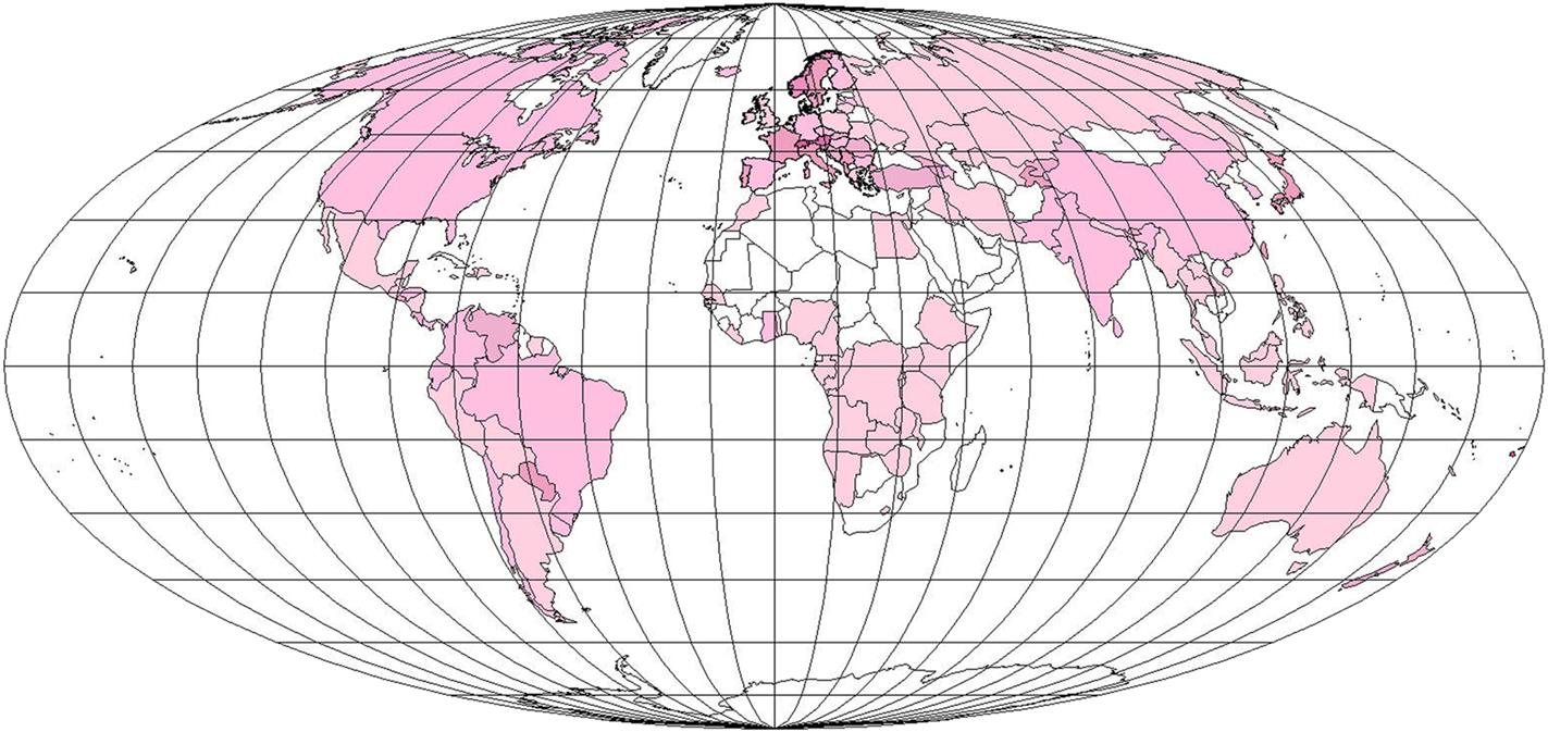
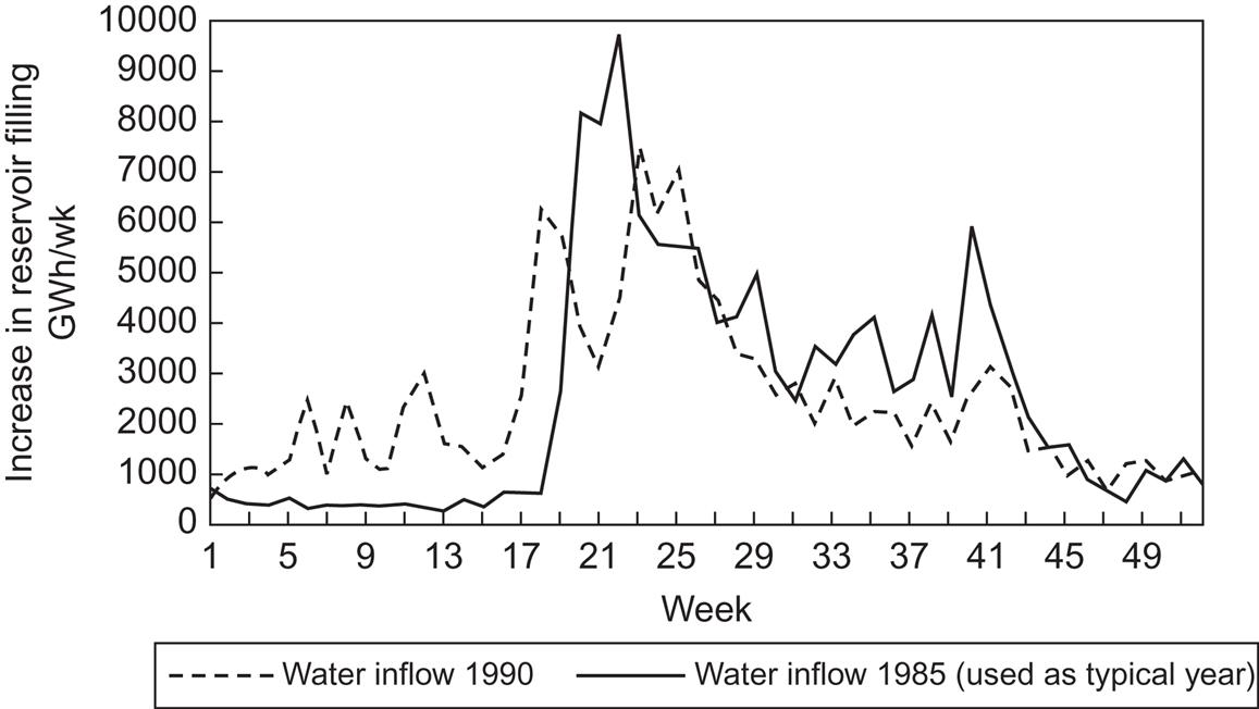
Figure 3.49 Hydropower potential average production (W m⁻²), including existing plants, plants under construction, and planned and contemplated installations, both for large- and small-scale power schemes. Based on data from World Energy Conference (1995).

Figure 3.50 gives seasonal variations (for 2 years) in the flow into the existing hydropower reservoirs in Norway, a country where the primary filling of reservoirs is associated with the melting of snow and ice during the late spring and early summer months.

Figure 3.50 Seasonal variation in the power associated with the water flow into Norwegian hydropower reservoirs for a typical year (1985) and a “dry year” (1990). Based on Andersen (1997); Meibom *et al*. (1999).

3.3.2.2 Environmental impact

The environmental impact of non-regulated hydro-generation of power is mainly interference with the migration of fish and other biota across the turbine area, but the building of dams in connection with large hydro facilities may have an even more profound influence on the ecology of the region, in addition to introducing accident risks. Large reservoirs have caused serious destruction of natural landscapes and dislocation of populations living in areas to be flooded as reservoirs. There are ways to avoid some of these problems. For example, in Switzerland, modular construction, where the water is cascaded through several smaller reservoirs, has made a substantial reduction in the area modified. Furthermore, reservoirs need not be constructed in direct connection with the generating plants, but can be separate installations placed in optimum locations, with a two-way turbine that uses excess electric production from other regions to pump water up into a high-lying reservoir. When other generating facilities cannot meet demand, the water is then released back through the turbine. This means that, although the water cycle may be unchanged on an annual average basis, considerable seasonal modifications of the hydrological cycle may be involved. The influence of such modifications on the vegetation and climate of the region below the reservoir, which would otherwise receive a water flow at a different time, has to be studied in each individual case. The upper region, as well, may experience modifications—for example, owing to increased evaporation in the presence of a full reservoir.

Although the modifications are local, their influence on the ecosystems can have serious consequences for man. A notable example is the Aswan Dam in Egypt, which has allowed aquatic snails to migrate from the Nile delta to upstream areas. The snails can carry parasites causing schistosomiasis, and the disease has actually spread from the delta region to Upper Egypt since the building of the dam (Hayes, 1977).

It is unlikely that hydropower utilization will ever be able to produce changes in the seasonal hydrological cycle, which could have global consequences, but no detailed investigation has yet been made. Such a study could resemble the investigation of the influence of deforestation, shown in Fig. 2.97.

The impacts of global warming include changes in the hydrological cycle (cf. Fig. 2.65). An analysis by Vliet et al. (2016) of the increases or decreases of water availability at the sites of current hydropower facilities suggests a reduction of around 2% of power production. For nuclear and fossil power plants depending on environmental cooling water, the loss of efficiency and hence output due to higher water temperatures will be larger, about 10%, but with possible mitigation options (using more water or different coolants).

3.3.3 Ocean waves

The order of magnitude of the total energy in wave motion is about 10⁻³ of the total kinetic energy in the atmospheric wind systems, according to the rough estimate made in section 2.4.1 in connection with Fig. 2.90. The wave energy of about 10 kJ m⁻² found as an annual average in the North Atlantic Ocean corresponds to the accumulated wind energy up to a height of about 200 m, according to Fig. 3.32. This implies that, although the amount of energy stored in waves is much smaller than the amount stored in wind, wave energy may still be equivalent to the height-integrated fraction of wind energy accessible for practical use, at least at the current level of technology.

From the tentative estimates in section 2.4.1, the average turnover time for the energy in wave motion in the open ocean may be of the order of a few days. This time is consistent with average dissipation mechanisms, such as internal friction and weak wave–wave interactions, plus shoreline dissipation modes. The input of energy by the wind, on the other hand, seems to be an intermittent process that, for extended intervals of time, involves only slow transfer of energy between waves and turbulent wind components, or vice versa, and between wind and wave fields propagating in different directions (any angle from 0 to 2π). However, large amounts of energy may be transferred from wind to waves during short periods of time (i.e., “short periods” compared with the average turnover time). This suggests that the energy storage in waves may be varying more smoothly than the storage in wind (both waves and wind represent short-term stored solar energy, rather than primary energy flows, as discussed in connection with Fig. 2.90). As mentioned in section 2.3.2, the wave fields exhibit short-term fluctuations, which may be regarded as random. On a medium time scale, the characteristics of the creation and dissipation mechanisms may make wave energy a more “dependable” energy source than wind energy, but on a seasonal scale, the variations in wind and wave energy are expected to follow each other (cf. the discussion topic III.2 in Part III).

3.3.3.1 Wave spectra

The energy spectrum F(k) of a random wave field is defined by (2.79). Since the wavelength (or wave number k) is very difficult to observe directly, it is convenient instead to express the spectrum in terms of the frequency,

$v = ω (k) / 2 π = 1 / T .$ $v = ω (k) / 2 π = 1 / T .$

The frequency is obtained from the period, T, which for a harmonic wave equals the zero-crossing period, i.e., the time interval between successive passages of the wave surface through the zero (average) height, in the same direction. The spectral distribution of energy, or energy spectrum when expressed in terms of frequency, F₁(v)=2πF₁(ω), is usually normalized to the total energy (Barnett and Kenyon, 1975), whereas the wave number-dependent spectrum F(k), defined in section 2.3.2, is normalized to the average potential energy. Thus,

$\int F_{1} (ω) d ω = W^{t o t a l} = 2 \int F (k) d k .$ $\int F_{1} (ω) d ω = W^{t o t a l} = 2 \int F (k) d k .$

Figure 3.51 shows a set of measured energy spectra, F₁, based on data from the Atlantic Ocean (Moskowitz, 1964). The wave fields selected were judged to correspond to fully developed waves, and data corresponding to the same wind speed at a height of 20 m were averaged in order to provide the spectra shown in the figure. The figure shows that the spectral intensity increases, and the frequency corresponding to the peak intensity decreases, with increasing wind speed.

Figure 3.51 Energy spectrum of waves estimated to be “fully developed” for the Atlantic Ocean (data have been grouped according to the wind speed at a height of 20 m). Based on Moskowitz (1964).

Based on the similarity theory of Monin and Obukhov (1954), Kitaigorodskii (1970) suggested that F₁(ω)g²ρ_w⁻¹V⁻⁵ (V being the wind speed) would be a universal function of ωVg⁻¹, with both quantities being dimensionless. Based on the data shown in Fig. 3.51, which approximately satisfy Kitaigorodskii’s hypothesis, Moskowitz (1964) suggested the following analytical form for the energy spectrum of fully developed gravity waves,

$F_{1} (ω) = 8.1 \times 10^{- 3} ρ_{w} g^{3} ω^{- 5} \exp (- 0.74 {(V {z = 20 m} ω / g)}^{- 4}) .$ $F_{1} (ω) = 8.1 \times 10^{- 3} ρ_{w} g^{3} ω^{- 5} \exp (- 0.74 {(V {z = 20 m} ω / g)}^{- 4}) .$ (3.27)

(3.27)

The usefulness of this relation is limited by its sensitivity to the wind speed at a single height and by the difficulty of determining whether a given wave field is fully developed.

If the wave field is “fetch-limited,” i.e., if the wind has been able to act over only a limited length, then the energy spectrum will peak at a higher frequency, and the intensity will be lower, as shown in Fig. 3.52. Hasselmann et al. (1973) have generalized (3.27) to situations in which the wave field is not necessarily fully developed, according to such data.

..................Content has been hidden....................

You can't read the all page of ebook, please click here login for view all page.

Table of Contents for 3. Individual renewable energy sources

Create new playlist

Sign In

Sign Up