
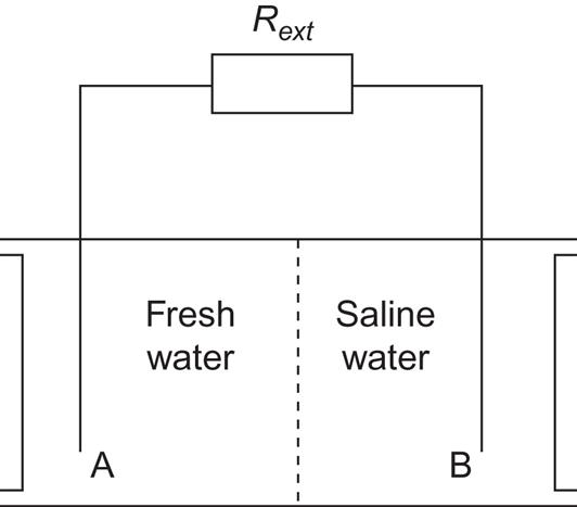
Inserting the numerical values given in section 3.7.2, and T=300 K, the cell electromotive force becomes ϕ≈0.05 V. The actual value of the external potential, Δϕext, may be reduced as a result of various losses, as described in section 4.5.1 (e.g., Fig. 4.105). ϕ is also altered if the “fresh” water has a finite amount of ions or if ions other than Na+ and Cl− are present.
If the load resistance is Rext, the power delivered by the cell is given by the current I=Δϕext Rext−1,
and, as usual, the maximum power corresponds to an external potential difference Δϕext, which is smaller than the open-circuit value (4.151). Internal losses may be represented by an internal resistance Rint, defined by
Thus, the power output may also be written
Rint depends on electrode properties, as well as on ![]() and nCl- and their variations across the cell.
and nCl- and their variations across the cell.
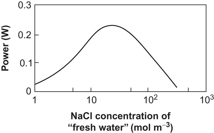
Several anode-membrane plus cathode-membrane units may be stacked beside each other in order to obtain a sufficiently large current (which is necessary because the total internal resistance has a tendency to increase strongly if the current is below a certain value). Figure 4.110 shows the results of a small-scale experiment (Weinstein and Leitz, 1976) for a stack of about 30 membrane-electrode pairs and an external load, Rext, close to the one giving maximum power output. The power is shown, however, as a function of the salinity of the fresh water, and it is seen that the largest power output is obtained for a fresh-water salinity that is not zero but 3–4% of the seawater salinity. The reason is that, although the electromotive force (4.151) diminishes with increasing fresh-water salinity, the decrease is at first more than compensated for by the improved conductivity of the solution (decrease in Rint) when ions are also initially present in the fresh-water compartment.
Needless to say, small-scale experiments of the kind described above are a long way from a demonstration of viability of the salinity gradient conversion devices on a large scale, and it is by no means clear whether the dialysis battery concept will be more or less viable than power turbines based on osmotic umps. The former seems likely to demand a larger membrane area than the latter, but no complete evaluation of design criteria has been made in either case.
4.6 Bioenergy conversion processes
A number of conversion processes aim at converting one fuel into another that is considered more versatile. Examples are charcoal production from wood (efficiency of conversion about 50%), liquefaction, and gasification (Squires, 1974). Figure 4.111 gives an overview of the non-food uses of biomass, to be discussed in more detail in the following.
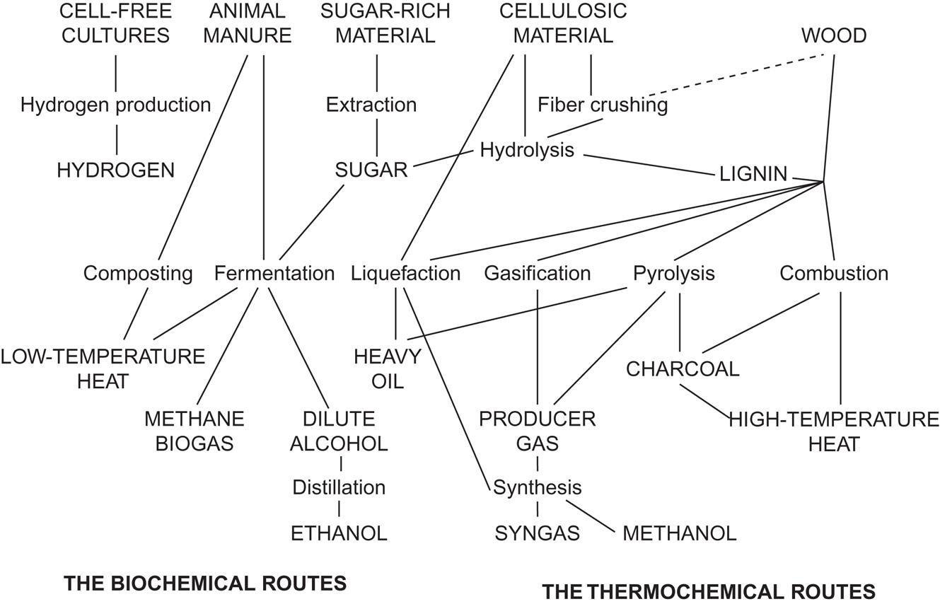
Fresh biomass is a large potential source of renewable energy that, in addition to use for combustion, may be converted into a number of liquid and gaseous biofuels. The conversion may be achieved by thermochemical or biochemical methods, as described below.
However, biomass is not just stored energy; it is also a store of nutrients and a potential raw material for a number of industries. Therefore, bioenergy is a topic that cannot be separated from food production, timber industries (serving construction purposes, paper and pulp industries, etc.), and organic feedstock-dependent industries (chemical and biochemical industries, notably). Furthermore, biomass is derived from plant growth and animal husbandry, linking the energy aspect to agriculture, livestock, silviculture, aquaculture, and quite generally to the management of the global ecological system. Thus, procuring and utilizing organic fuels constitute a profound interference with the natural biosphere, and understanding the range of impacts as well as elimination of unacceptable ones should be an integral part of any scheme for diversion of organic fuels to human society.
4.6.1 Combustion and composting of biomass
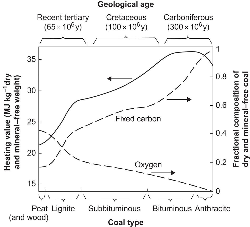
Traditional uses of organic fuels as energy carriers comprise the use of fresh biomass, i.e., storage and combustion of wood fuels, straw, and other plant residues, and, in recent centuries, notably storage and combustion of fossilized biomass, i.e., fuels derived from coal, oil, and natural gas. While the energy density of living biomass is in the range of 10–30 MJ per kg of dry weight, several million years of fossilization processes typically increase the energy density by a factor of 2 (see Fig. 4.112). The highest energy density is found for oil, where the average density of crude oil is 42 MJ kg−1.
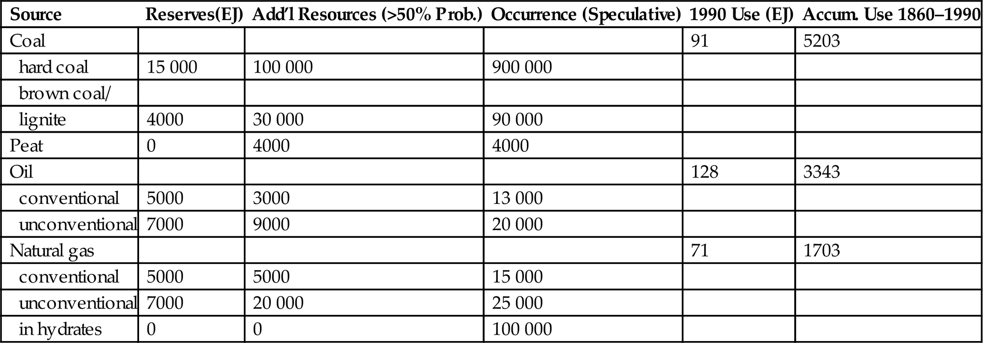
The known reserves of fossil fuels that may be economically extracted today, and estimates of further resources exploitable at higher costs, are indicated in Table 4.2. The finiteness of such resources is, of course, together with the environmental impact issues, the reason for turning to renewable energy sources, including renewable usage of biomass resources.
Table 4.2
Fossil reserves, additional resources, and consumption in EJ (UN, 1981; Jensen and Sørensen, 1984; Nakicenovic et al., 1996).
| Source | Reserves(EJ) | Add’l Resources (>50% Prob.) | Occurrence (Speculative) | 1990 Use (EJ) | Accum. Use 1860–1990 |
| Coal | 91 | 5203 | |||
| hard coal | 15 000 | 100 000 | 900 000 | ||
| brown coal/ | |||||
| lignite | 4000 | 30 000 | 90 000 | ||
| Peat | 0 | 4000 | 4000 | ||
| Oil | 128 | 3343 | |||
| conventional | 5000 | 3000 | 13 000 | ||
| unconventional | 7000 | 9000 | 20 000 | ||
| Natural gas | 71 | 1703 | |||
| conventional | 5000 | 5000 | 15 000 | ||
| unconventional | 7000 | 20 000 | 25 000 | ||
| in hydrates | 0 | 0 | 100 000 |
Traditionally, fossil fuels used for combustion in industry, power generation, and transportation have been large contributors of health-damaging emissions. This and the CO2 emissions causing climate change will be dealt with in Chapter 7 by life-cycle analysis. Because viable alternatives and notably renewable energy supply with proper handling of intermittency (Sørensen, 2015) are now available, fossil fuels can and should be phased out even if there are resources left. Some of these may be useful for non-energy purposes in the future (lubricants, etc.). In particular, the low-grade resources such as inferior coal, oil shale, and tar sands should be avoided, due to the extreme pollution of soils and waterways caused by extraction. Even organic aerosol emissions during exploitation and refining seem unavoidable (Liggio et al., 2016).
The proponents of using fossil sources for energy until final exhaustion have suggested capturing the produced CO2 before emission, which leaves a problem of where to deposit the captured CO2. Because of the enormous quantities involved (44 molecular mass units for each 12 units of carbon), deposition in abandoned mines and similar dumps is grossly insufficient, and only deep ocean disposal appears viable, if long-tern stability of the sites can be proven. The capture of CO2 from the flue gas stream is costly and inefficient, and research is still ongoing on finding new avenues (McDonald et al., 2015). An alternative would be to shift the energy from, for example, natural gas or coal to hydrogen by a suitable process, again with CO2 as a byproduct (Sørensen, 2012), considering that hydrogen may have several uses in the future (if fuel cells become viable) and that the efficiency is higher than extraction of CO2 from stack gas. As regards the final disposal of CO2 in oceans, the hope is that certain deep locations would permit plain dumping and yet have little chance that the CO2 moves away before being incorporated into chalk-like substances (Matter et al., 2016). The most likely conclusion is that these efforts will remain expensive in terms of both energy inputs and cost.
4.6.1.1 Producing heat by burning biomass
Heat may be obtained from biological materials by burning, eventually with the purpose of further conversion. Efficient burning usually requires the reduction of water content, for example, by sun-drying. The heat produced by burning cow dung is about 1.5×10⁷ J per kg of dry matter, but initially only about 10% is dry matter, so the vaporization of 9 kg of water implies an energy requirement of 2.2×10⁷ J, i.e., the burning process is a net energy producer only if substantial sun-drying is possible. Firewood and other biomass sources constitute stores of energy, since they can be dried during the summer and used during winter periods when the heating requirement may be large and the possibility of sun-drying may not exist. The heat produced by burning 1 kg of dry wood or sawmill scrap is about 1.25×10⁷ J (1 kg in these cases corresponds to a volume of approximately 1.5×10⁻³ m3), and the heat from burning 1 kg of straw (assumed water content 15%) is about 1.5×10⁷ J (Eckert, 1960). Boilers used for firing with wood or straw have efficiencies that are often considerably lower than those of oil or gas burners. Typical efficiencies are in the range 0.5–0.6 for the best boilers. The rest of the enthalpy is lost, mostly in the form of vapor and heat leaving the chimney (or other smoke exit), and therefore is not available at the load area.
Combustion is the oxidation of carbon-containing material in the presence of sufficient oxygen to complete the process
Wood and other biomass is burned for cooking, for space heating, and for a number of specialized purposes, such as provision of process steam and electricity generation. In rural areas of many Third World countries, a device consisting of three stones for outdoor combustion of twigs is still the most common. In the absence of wind, up to about 5% of the heat energy may reach the contents of the pot resting on top of the stones. In some countries, indoor cooking on simple chulas is common. A chula is a combustion chamber with a place for one or more pots or pans on top, resting in such a way that the combustion gases will pass along the outer sides of the cooking pot and leave the room through any opening. Indoor air quality is extremely poor when chulas are in use, and village women in India using chulas for several hours each day are reported to suffer from severe cases of eye irritation and respiratory diseases (Vohra, 1982).
Earlier, most cooking in Europe and its colonies was done on stoves made of cast iron. These stoves, usually called European stoves, had controlled air intake and both primary and secondary air inlets, chimneys for regulation of gas passage, and several cooking places with ring systems allowing the pots to fit tightly in holes, with a part of the pot indented into the hot gas stream. The efficiency was up to about 25%, counted as energy delivered to the pots divided by wood energy spent, but such efficiency would only be reached if all holes were in use and if the different temperatures prevailing at different boiler holes could be made useful, including after-heat. In many cases, the average efficiency would hardly have exceeded 10%, but, in many of the areas in question, the heat lost to the room could also be considered useful, in which case close to 50% efficiency (useful energy divided by input) could be reached. Today, copies of the European stove are being introduced in several regions of the Third World, with the stoves constructed from local materials, such as clay and sand–clay mixtures, instead of cast iron.
Wood-burning stoves and furnaces for space heating have conversion efficiencies from below or about 10% (open furnace with vertical chimney) up to 50% (oven with two controlled air inlets and a labyrinth-shaped effluent gas route leading to a tall chimney). Industrial burners and stokers (for burning wood scrap) typically reach efficiencies of about 60%. Higher efficiencies require a very uniform fuel without variations in water content or density.
Most biological material is not uniform, and pretreatment can often improve both the transportation and storage processes and the combustion (or other final use). Irregular biomass (e.g., twigs) can be chopped or cut to provide unit sizes fitting the containers and burning spaces provided. Furthermore, compressing and pelletizing the fuel can make it considerably more versatile. For some time, straw compressors and pelletizers have been available, so that bulky straw bundles can be transformed into a fuel with volume densities approaching that of coal. Other biomass material can conceivably be pelletized advantageously, including wood scrap, mixed biomass residues, and even aquatic plant material (Anonymous, 1980). Portable pelletizers are available (e.g., in Denmark) that allow straw to be compressed in the growing fields, so that longer transport becomes economically feasible and so that even long-term storage (seasonal) of straw residues becomes attractive.
A commonly practiced conversion step is from wood to charcoal. Charcoal is easier to store and to transport. Furthermore, charcoal combustion—for example, for cooking—produces less visible smoke than direct wood burning and is typically so much more efficient than wood burning that, despite wood-to-charcoal conversion losses, less primary energy is used to cook a given meal with charcoal than with wood.
Particularly in rich countries, a considerable source of biomass energy is urban refuse, which contains residues from food preparation and discarded consumer goods from households, as well as organic scrap material from commerce and industry. Large-scale incineration of urban refuse has become an important source of heat, particularly in Western Europe, where it is used mainly for district heating (Renzo, 1978).
For steam generation purposes, combustion is performed in the presence of an abundant water source (waterwall incineration). In order to improve pollutant control, fluidized bed combustion techniques may be utilized (Cheremisinoff et al., 1980). The bed consists of fine-grain material, for example, sand, mixed with material to be burned (sawdust is particularly suitable, but any other biomass, including wood, can be accepted if finely chopped). The gaseous effluents from combustion, plus air, fluidize the bed as they pass through it under agitation. The water content of the material in the bed may be high (in which case steam production occurs). Combustion temperatures are lower than for flame burning, and this partly makes ash removal easier and partly reduces tar formation and salt vaporization. As a result, reactor life is extended and air pollution can better be controlled.
In general, the environmental impacts of biomass utilization through combustion may be substantial and comparable to, although not entirely of the same nature as, the impacts from coal and oil combustion (see Table 4.3). In addition, ashes will have to be disposed of. For boiler combustion, the sulfur dioxide emissions are typically much smaller than for oil and coal combustion, which would give 15–60 kg t−1 in the absence of flue gas cleaning. If ash is re-injected into the wood burner, higher sulfur values appear, but these values are still below the fossil-fuel emissions in the absence of sulfur removal efforts.
Table 4.3
Uncontrolled emissions from biomass combustion in boilers (kg per ton of fuel, based on woody biomass; US EPA, 1980)
| Substance Emitted | Emissions (kg/103 kg) |
| Particulates | 12.5−15.0 |
| Organic compoundsa | 1.0 |
| Sulfur dioxide | 0−1.5b |
| Nitrogen oxides | 5.0 |
| Carbon monoxide | 1.0 |
aHydrocarbons including methane and traces of benzo(a)pyrine.
bUpper limit is found for bark combustion. Ten times higher values are reported in cases where combustion ashes are re-injected.
Particulates are not normally regulated in home boilers, but for power plants and industrial boilers, electrostatic filters are employed, with particulate removal up to over 99%. Compared to coal burning without particle removal, wood emissions are 5–10 times lower. When a wood boiler is started, there is an initial period of very visible smoke emission, consisting of water vapor and high levels of both particulate and gaseous emissions. After the boiler reaches operating temperatures, wood burns virtually without visible smoke. When stack temperatures are below 60°C, during start-up and during incorrect burning, severe soot problems arise.
Nitrogen oxide emissions are typically 2–3 times lower for biomass burning than for coal burning (per kilogram of fuel), but often similar emissions occur per unit of energy delivered.
Particular concern should be directed at organic-compound emissions from biomass burning. In particular, benzo(a)pyrene emissions from biomass are found to be up to 50 times higher than for fossil-fuel combustion, and the measured concentrations of benzo(a)pyrene in village houses in Northern India (1.3–9.3×10⁻⁹ kg m−3), where primitive wood-burning chulas are used for several (6–8) hours every day, exceed German standards of 10−11 kg m−3 by 2–3 orders of magnitude (Vohra, 1982). However, boilers with higher combustion temperatures largely avoid this problem, as indicated in Table 4.3.
The lowest emissions are achieved if batches of biomass are burned at optimal conditions, rather than regulating the boiler up and down according to heating load. Therefore, wood heating systems consisting of a boiler and a heat storage unit (gravel, water) with several hours of load capacity will lead to the smallest environmental problems (Hermes and Lew, 1982). This example shows that there can be situations where energy storage would be introduced entirely for environmental reasons.
The occupational hazards that arise during tree felling and handling should be mentioned. The accident rate among forest workers is high in many parts of the world, and safer working conditions for forest workers are imperative if wood is to be used sensibly for fuel applications.
Finally, although CO2 accumulates in the atmosphere as a consequence of fossil fuel combustion, CO2 emissions during biomass combustion are balanced in magnitude by the CO2 assimilation by plants, so that the atmospheric CO2 content is not affected, at least by the use of biomass crops in fast rotation. However, the lag time, e.g., for trees, may be decades or centuries, and, in such cases, temporary CO2 imbalance may contribute to climatic alterations.
4.6.1.2 Composting
Primary organic materials form the basis for a number of energy conversion processes other than burning. Since they produce liquid or gaseous fuels, plus associated heat, they are dealt with in the following sections on fuel production. However, conversion aiming directly at heat production has also been utilized, with non-combustion processes based on manure from livestock animals and in some cases on primary biomass residues.
Two forms of composting are in use, one based on fluid manure (less than 10% dry matter), and the other based on solid manure (50–80% dry matter). In both cases, the chemical process is bacterial decomposition under aerobic conditions, i.e., the compost heap or container has to be ventilated in order to provide a continuous supply of oxygen for the bacterial processes. The bacteria required for the process (of which lactic acid producers constitute the largest fraction; cf. McCoy, 1967) are normally all present in manure, unless antibiotic residues that kill bacteria are retained after some veterinary treatment. The processes involved in composting are very complex, but it is believed that decomposition of carbohydrates [the inverse of reaction (3.45)] is responsible for most of the heat production (Popel, 1970). A fraction of the carbon from the organic material is found in new-bred microorganisms.
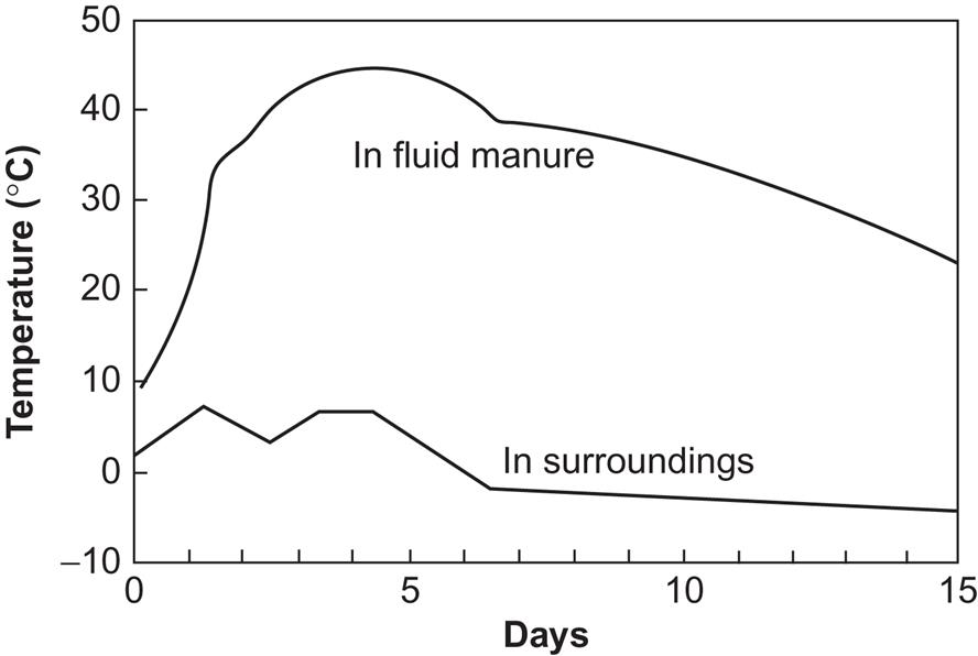
A device for treating fluid manure may consist of a container with a blower injecting fresh air into the fluid in such a way that it becomes well distributed over the fluid volume. An exit air channel carries the heated airflow to, say, a heat exchanger. Figure 4.113 shows an example of the temperature of the liquid manure, along with the temperature outside the container walls, as a function of time. The amount of energy required for the air blower is typically around 50% of the heat energy output, and is in the form of high-quality mechanical energy (e.g., from an electrically driven rotor). Thus, the simple efficiency may be around 50%, but the second law efficiency (4.20) may be quite low.
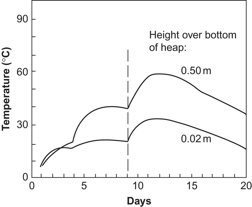
Heat production from solid manure follows a similar pattern. The temperature in the middle of a manure heap (dunghill) may be higher than that of liquid manure, owing to the low heat capacity of the solid manure (see Fig. 4.114). Air may be supplied by blowers placed at the bottom of the heap, and, in order to maintain air passage space inside the heap and remove moisture, occasional re-stacking of the heap is required. A certain degree of variation in air supply can be allowed, so that the blower may be driven by a renewable energy converter, for example, a windmill, without storage or back-up power. With frequent re-stacking, air supply by blowing is not required, but the required amount of mechanical energy input per unit of heat extraction is probably as high as for liquid manure. In addition, the heat extraction process is more difficult, demanding, for example, that heat exchangers be built into the heap itself (water pipes are one possibility). If an insufficient amount of air is provided, the composting process will stop before the maximum heat has been obtained.
Owing to the bacteriological decomposition of most of the large organic molecules present, the final composting product has considerable value as fertilizer.
4.6.1.3 Metabolic heat
Metabolic heat from the life processes of animals can also be used by man, in addition to the heating of human habitats by man’s own metabolic heat. A livestock shed or barn produces enough heat, under most conditions of winter occupancy, to cover the heating requirements of adjacent farm buildings, in addition to providing adequate temperature levels for the animals. One reason for this is that livestock barns must have a high rate of ventilation in order to remove dust (e.g., from the animal’s skin, fur, hair, or feathers) and water vapor. Therefore, utilization of barn heat may not require extra feeding of the animals, but may simply consist of heat recovery from air that for other reasons has to be removed. Utilization for heating a nearby residence building often requires a heat pump (see section 4.6.1), because the temperature of the ventilation air is usually lower than that required at the load area, and a simple heat exchanger would not work.
In temperate climates, the average temperature in a livestock shed or barn may be about 15°C during winter. If young animals are present, the required temperature is higher. With an outside temperature of 0°C and no particular insulation of walls, the net heat production of such barns or sheds is positive when the occupants are fully grown animals, but negative if the occupants are young individuals and very much so if newborn animals are present (Olsen, 1975). In chicken or pig farms, the need for heat input may be avoided by having populations of mixed age or heat exchange between compartments for young and adult animals. The best candidates for heat extraction to other applications might then be dairy farms.
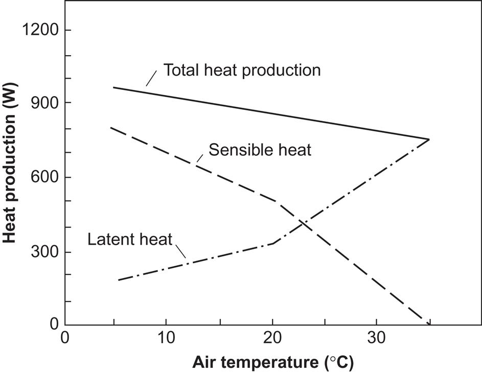
A dairy cow transfers about 25% of the chemical energy in fodder to milk and a similar amount to manure (Claesson, 1974). If the weight of the cow remains constant, the rest is converted to heat and is rejected as heat radiation, convection, or latent heat of water vaporization. The distribution of the heat production in sensible and latent forms of heat is indicated in Fig. 4.115. It is strongly dependent on the air temperature in the barn. At 15°C, about two-thirds of the heat production is in the form of sensible heat. Heat transfer to a heat pump circuit may take place from the ventilation air exit. Water condensation on the heat exchanger surface involved may help to prevent dust particles from accumulating on the heat exchanger surface.
4.6.2 Biological conversion into gaseous fuels
Fuels are biological material (including fossilized forms), hydrocarbons, or just hydrogen, which can be stored and used at convenient times. Usage traditionally means burning in air or pure oxygen, but other means of conversion exist, for example, fuel cells (see section 4.5).
Before discussing the conversion of fresh biomass, the gasification of coal is briefly discussed because of its importance for possible continued use of fossil biomass (coal being the largest such source) and also because of its similarity to processes relevant for other solid biomass.
Inefficient conversion of gasified coal to oil has historically been used by isolated coal-rich but oil-deficient nations (Germany during World War II, South Africa). Coal is gasified to carbon monoxide and hydrogen, which is then, by the Fischer-Tropsch process (passage through a reactor, e.g., a fluidized bed, with a nickel, cobalt, or iron catalyst), partially converted into hydrocarbons. Sulfur compounds have to be removed because they would impede the function of the catalyst. The reactions involved are of the form
and conversion efficiencies range from 21% to 55% (Robinson, 1980). Further separation of the hydrocarbons generated may then be performed; for instance, gasoline corresponding to the range 4 ≤ n ≤ 10 in the above formulae.
Alternative coal liquefaction processes involve direct hydrogenation of coal under suitable pressures and temperatures. Pilot plants have been operating in the United States, producing up to 600 t a day (slightly different processes are named solvent refining, H-coal process, and donor solvent process; cf. Hammond, 1976). From an energy storage point of view, either coal or the converted product may be stockpiled.
For use in the transportation sector, production of liquid hydrocarbons, such as ethanol, methanol, and diesel-like fluids, is considered. The liquid hydrocarbons can be produced from fossil or renewable biomass sources as described below, often with thermochemical gasification as the first conversion step.
4.6.2.1 Biogas
Conversion of (fresh) biological material into simple hydrocarbons or hydrogen can be achieved by a number of anaerobic fermentation processes, i.e., processes performed by suitable microorganisms and taking place in the absence of oxygen. The anaerobic “digestion” processes work on most fresh biological material, wood excepted, provided that proper conditions are maintained (temperature, population of microorganisms, stirring, etc.). Thus, biological material in forms inconvenient for storage and use may be converted into liquid or gaseous fuels that can be utilized in a multitude of ways, like oil and natural gas products.
The “raw materials” that may be used are slurry or manure (e.g., from dairy farms or “industrial farming” involving large feedlots), city sewage and refuse, farming crop residues (e.g., straw or parts of cereal or fodder plants not normally harvested), or direct “fuel crops,” such as ocean-grown algae or seaweeds, water hyacinths (in tropical climates), or fast-growing bushes or trees. The deep harvesting necessary to collect crop residues may not be generally advisable, owing to the role of these residues in preventing soil erosion.
Among the fermentation processes, one set is particularly suited for producing gas from biomass in a wet process (cf. Fig. 4.111). It is called anaerobic digestion. It traditionally used animal manure as biomass feedstock, but other biomass sources can be used within limits that are briefly discussed in the following. The set of biochemical reactions making up the digestion process (a term indicating the close analogy to energy extraction from biomass by food digestion) is schematically illustrated in Fig. 4.116.
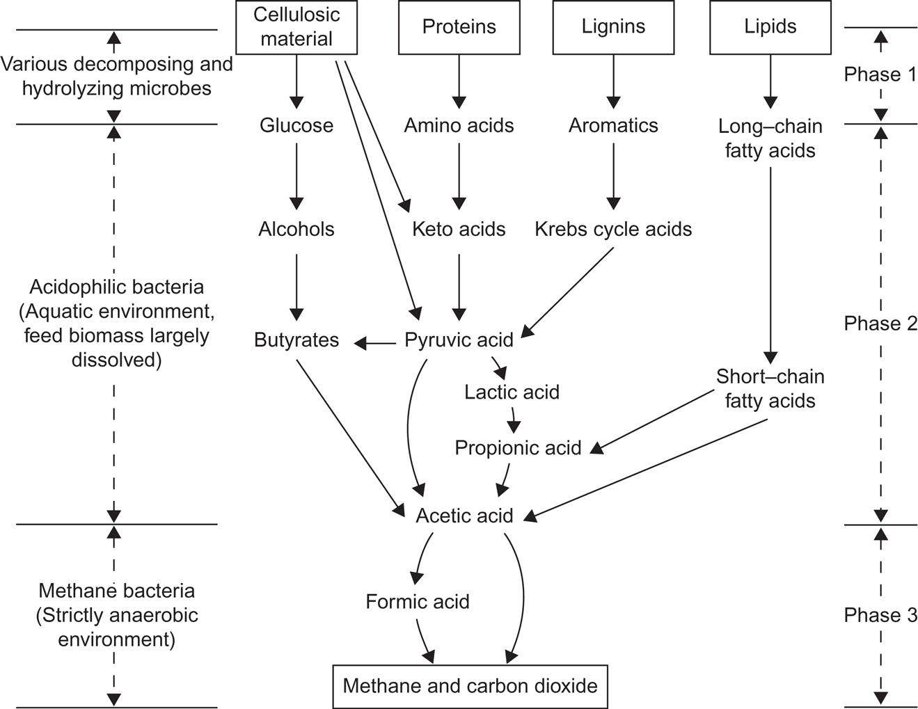
Anaerobic digestion has three discernible stages. In the first, complex biomass material is decomposed by a heterogeneous set of microorganisms, not necessarily confined to anaerobic environments. These decompositions comprise hydrolysis of cellulosic material to simple glucose, using enzymes provided by the microorganisms as catalysts. Similarly, proteins are decomposed to amino acids and lipids to long-chain fatty acids. The significant result of the first stage is that most of the biomass is now water-soluble and in a simpler chemical form, suited for the next stage.
The second stage involves dehydrogenation (removing hydrogen atoms from the biomass material), such as changing glucose into acetic acid, carboxylation (removing carboxyl groups) of amino acids, and breakdown of the long-chain fatty acids into short-chain acids, again obtaining acetic acid as the final product. These reactions are fermentation reactions accomplished by a range of acidophilic (acid-forming) bacteria. Their optimum performance requires an environmental pH of 6–7 (slightly acid), but because the acids already formed will lower the pH of the solution, it is sometimes necessary to adjust the pH (e.g., by adding lime).
Finally, the third stage is the production of biogas (a mixture of methane and carbon dioxide) from acetic acid by a second set of fermentation reactions performed by methanogenic bacteria. These bacteria require a strictly anaerobic (oxygen-free) environment. Often, all processes are made to take place in a single container, but separation of the processes into stages allows greater efficiencies to be reached. The third stage takes on the order of weeks, while the preceding stages take on the order of hours or days, depending on the nature of the feedstock.
Starting from cellulose, the overall process may be summarized as
(4.152)
The first-stage reactions add up to
(4.153)
The net result of the second-stage reactions is
(4.154)
with intermediate steps, such as
(4.155)
followed by dehydrogenation:
(4.156)
The third-stage reactions then combine to
(4.157)
In order for the digestion to proceed, a number of conditions must be fulfilled. Bacterial action is inhibited by the presence of metal salts, penicillin, soluble sulfides, or ammonia in high concentrations. Some source of nitrogen is essential for the growth of the microorganisms. If there is too little nitrogen relative to the amount of carbon-containing material to be transformed, then bacterial growth is insufficient and biogas is production low. With too much nitrogen (a carbon–nitrogen ratio below 15), “ammonia poisoning” of the bacterial cultures may occur. When the carbon–nitrogen ratio exceeds about 30, gas production starts diminishing, but in some systems carbon–nitrogen values as high as 70 have prevailed without problems (Stafford et al., 1981). Table 4.4 gives carbon–nitrogen values for a number of biomass feedstocks. It is seen that mixing feedstocks can often be advantageous. For instance, straw and sawdust would have to be mixed with some low C:N material, such as livestock urine or clover/lucerne (typical secondary crops that may be grown in temperate climates after the main harvest).
Table 4.4
Carbon–nitrogen ratios for various materials.
| Material | Ratio |
| Sewage sludge | 13:1 |
| Cow dung | 25:1 |
| Cow urine | 0.8:1 |
| Pig droppings | 20:1 |
| Pig urine | 6:1 |
| Chicken manure | 25:1 |
| Kitchen refuse | 6−10:1 |
| Sawdust | 200−500:1 |
| Straw | 60−200:1 |
| Bagasse | 150:1 |
| Seaweed | 80:1 |
| Alfalfa hay | 18:1 |
| Grass clippings | 12:1 |
| Potato tops | 25:1 |
| Silage liquor | 11:1 |
| Slaughterhouse wastes | 3−4:1 |
| Clover | 2.7:1 |
| Lucerne | 2:1 |
Source: Based on Baader et al. (1978); Rubins and Bear (1942).
If digestion time is not a problem, almost any cellulosic material can be converted to biogas, even pure straw. Initially, one may have to wait for several months, until the optimum bacterial composition has been reached, but then continued production can take place, and, despite low reaction rates, an energy recovery similar to that of manure can be achieved with properly prolonged reaction times (Mardon, 1982).
Average manure production for fully-grown cows and pigs (in Europe, Australia, and the Americas) is 40 and 2.3 kg wet weight d−1, respectively, corresponding to 62 and 6.2 MJ d−1, respectively. The equivalent biogas production may reach 1.2 and 0.18 m3 d−1. This amounts to 26 and 3.8 MJ d−1, or 42% and 61% conversion efficiency, respectively (Taiganides, 1974). A discussion of the overall efficiency, including transportation of biomass to the production plant, is given in Berglund and Börjesson (2002), who found maximum acceptable transport distances of 100–150 km.
The residue from the anaerobic digestion process has a higher value as a fertilizer than the feedstock. Insoluble organics in the original material are, to a large extent, made soluble, and nitrogen is fixed in the microorganisms.
Pathogen populations in the sludge are reduced. Stafford et al. (1981) found a 65–90% removal of Salmonella during anaerobic fermentation, and there is a significant reduction in streptococci, coliforms, and viruses, as well as an almost total elimination of disease-transmitting parasites like Ascaris, hookworm, Entamoeba, and Schistosoma.
For this reason, anaerobic fermentation has been used fairly extensively as a cleaning operation in city sewage treatment plants, either directly on the sludge or after algae are grown on the sludge to increase fermentation potential. Most newer sewage treatment plants make use of the biogas produced to fuel other parts of the treatment process, but, with proper management, sewage plants may well be net energy producers (Oswald, 1973). Biogas has been used as a (farm and road) vehicle fuel, using compressed gas flasks. The status and future prospects seem positive, but only few countries have yet established the required infrastructure (Jensen and Sørensen, 1984; Börjesson and Mathiasson, 2007).
The other long-time experience with biogas and associated fertilizer production is in rural areas of a number of Asian countries, notably China and India. The raw materials here are mostly cow dung, pig slurry, and human waste that is referred to as night soil, plus in some cases grass and straw. The biogas is used for cooking, and the fertilizer residue is returned to the fields. The sanitary aspect of pathogen reduction lends strong support to the economic viability of these schemes.
The rural systems are usually based on simple one-compartment digesters with human labor for filling and emptying of material. Operation is either in batches or with continuous new feed and removal of some 3–7% of the reactor content every day. Semi-industrialized plants have also been built during the last decade, for example, in connection with large pig farms, where mechanized and highly automated collection of manure has been feasible. In some cases, these installations have utilized separate acid and methanation tanks.
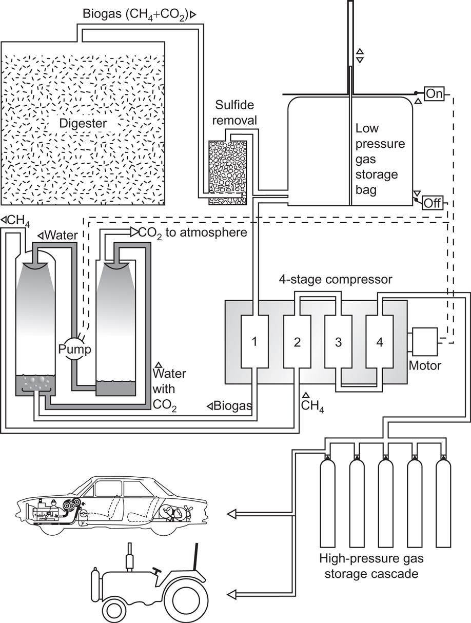
Figure 4.117 shows an example of a town-scale digester plant, where the biogas is used in a combined electric power and district heat-generating plant (Kraemer, 1981). Expected energy flows are indicated. Storage of biogas for rural cooking systems is accomplished by variable-volume domes that collect the gas as it is produced (e.g., an inverted, water-locked can placed over the digester core). Biogas contains approximately 23 MJ m−3 and is therefore a medium-quality gas. CO2 removal is necessary in order to achieve pipeline quality. An inexpensive way of achieving over 90% CO2 removal is by water spraying. This method of producing compressed methane gas from biogas allows for automotive applications, such as a farmer producing his tractor fuel on site. In New Zealand, such uses have been developed since 1980 (see Fig. 4.118; Stewart and McLeod, 1980). Several demonstration experiences have recently been undertaken in Sweden (Losciale, 2002).
Storage of a certain amount of methane at ambient pressure requires over a thousand times more volume than the equivalent storage of oil. However, actual methane storage at industrial facilities uses pressures of about 140 times ambient (Biomass Energy Institute, 1978), so the volume penalty relative to oil storage would then be a factor of nine. Storage of methane in zeolitic material for later use in vehicles has been considered.
If residues are recycled, little environmental impact can be expected from anaerobic digestion. The net impact on agriculture may be positive, owing to nutrients being made more accessible and due to parasite depression. Undesirable contaminants, such as heavy metals, are returned to the soil in approximately the same concentrations as existed before collection, unless urban pollution has access to the feedstock. The very fact that digestion depends on biological organisms may mean that poor digester performance could serve as a warning signal, directing early attention to pollution of cropland or urban sewage systems. In any case, pollutant-containing waste, for example, from industry, should never be mixed with the energy-valuable biological material in urban refuse and sewage. Methane-forming bacteria are more sensitive to changes in their environment, such as temperature and acidity, than are acid-forming bacteria.
The digestion process itself does not emit pollutants if it operates correctly, but gas cleaning, such as H2S removal, may lead to emissions. The methane gas itself shares many of the safety hazards of other gaseous fuels, being asphyxiating and explosive at certain concentrations in air (roughly 7–14% by volume). For rural cooking applications, the risks may be compared with those of the fuels being replaced by biogas, notably wood burned in simple stoves. In these cases, as follows from the discussion in section 4.6.1, the environment is dramatically improved by the introduction of biogas digesters.
An example of early biogas plants for use on a village scale in China, India, and Pakistan is shown in Fig. 4.119. All the reactions take place in one compartment, which does not necessarily lead to optimal conversion efficiency. The time required for the acid-forming step is less than 24 h, whereas the duration of the second step should be 10–30 days. In many climatic regions, the heating of the fermentation tank required for application may be done by solar collectors, which could form the top cover of the tank. Alternatively, the top cover may be an inflatable dome serving as a store of gas, which can smooth out a certain degree of load variation. Some installations obtain the highest efficiency by batch operation, i.e., by leaving one batch of biological material in the tank for the entire fermentation period. The one shown in Fig. 4.119 allows continuous operation, i.e., a fraction of the slurry is removed every day and replaced by fresh biological material.

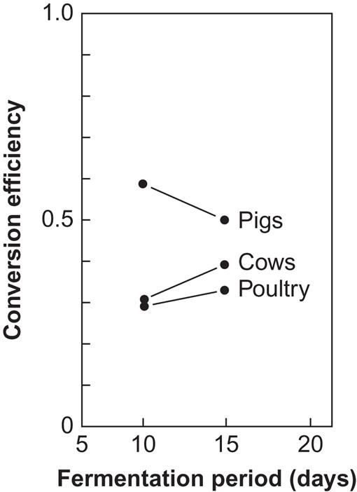
Examples of predicted biogas production rates, for simple plants of the type shown in Fig. 4.119 and based on fluid manure from dairy cows, pigs, or poultry, are shown in Table 4.5 and Fig. 4.120. Table 4.5 gives typical biogas production rates, per day and per animal, while Fig. 4.120 gives the conversion efficiencies measured, as functions of fermentation time (tank residence time), in a controlled experiment. The conversion efficiency is the ratio of the energy in the biogas (approximately 23 MJ m−3 of gas) and the energy in the manure that would be released as heat by complete burning of the dry matter (some typical absolute values are given in Table 4.5). The highest efficiency is obtained with pigs’ slurry, but the high bacteriological activity in this case occasionally has the side-effect of favoring bacteria other than those helping to produce biogas, e.g., ammonia-producing bacteria, the activity of which may destroy the possibility of further biogas production (Olsen, 1975).
Table 4.5
Manure and potential biogas production for a typical animal per day.
| Source | Manure Per Day | Biogas Per Day | ||
| kg Wet Weight | MJ | m3 | MJ | |
| Cows | 40 | 62 | 1.2 | 26 |
| Pigs | 2.3 | 6.2 | 0.18 | 3.8 |
| Hens | 0.19 | 0.9 | 0.011 | 0.26 |
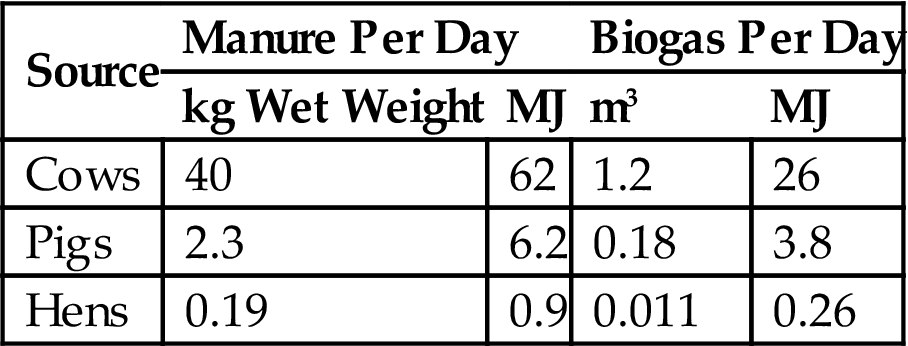
Source: Based on Taiganides (1974).
As mentioned, the manure residue from biogas plants has a high value as fertilizer because the decomposition of organic material followed by hydrocarbon conversion leaves plant nutrients (e.g., nitrogen that was originally bound in proteins) in a form suitable for uptake. Pathogenic bacteria and parasites are not removed to as high a degree as by composting, owing to the lower process temperature.
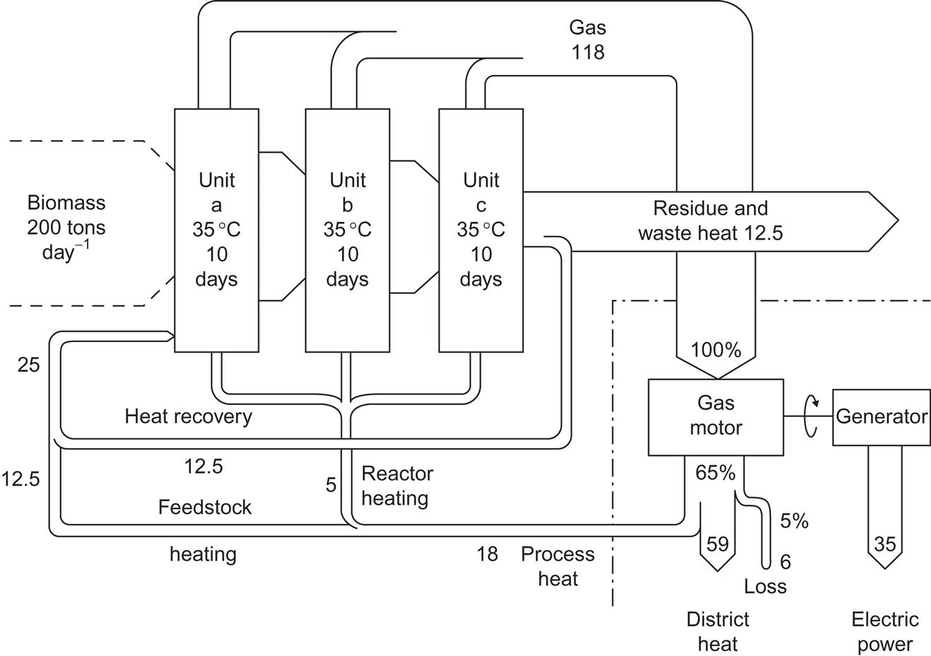
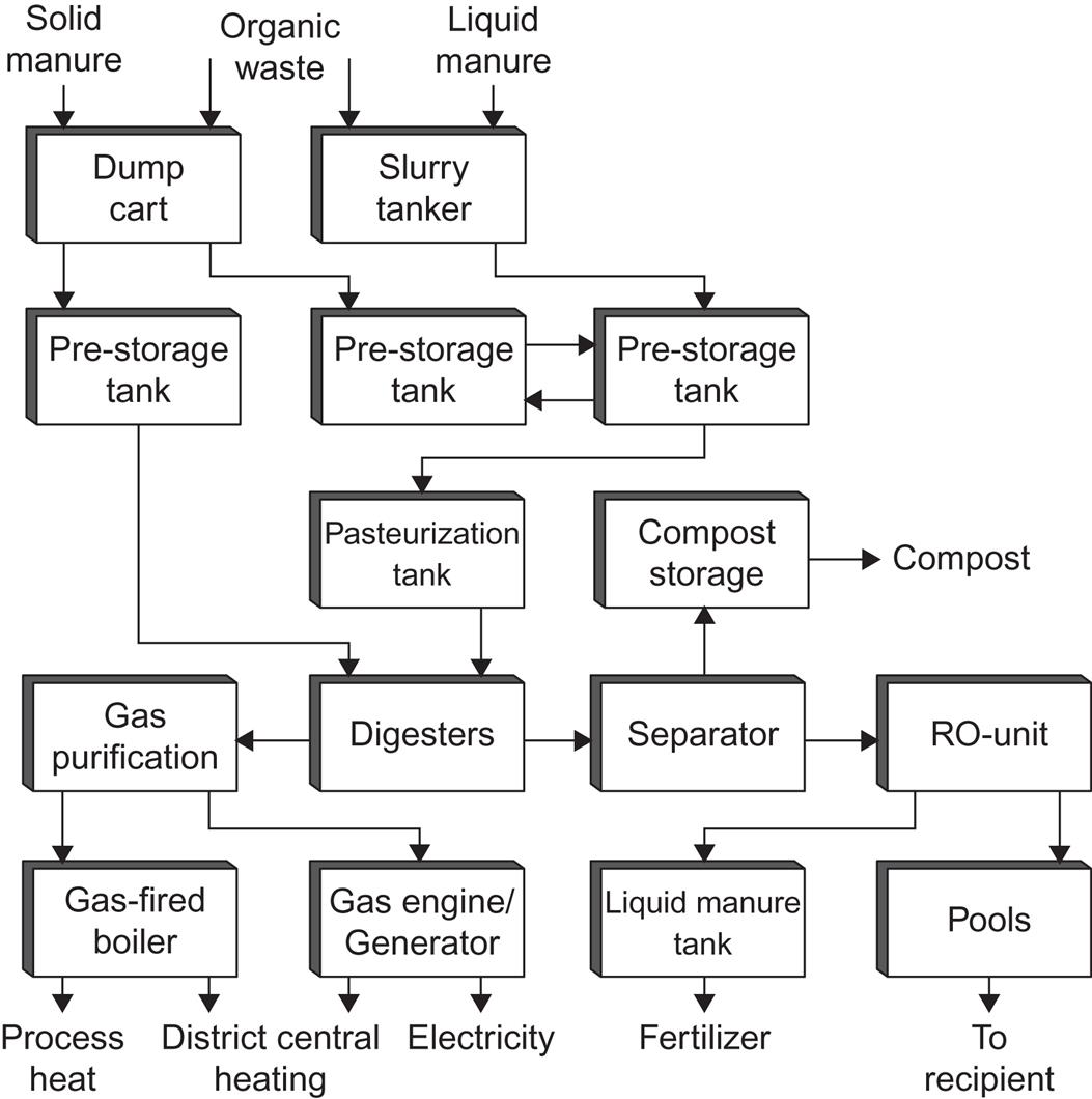
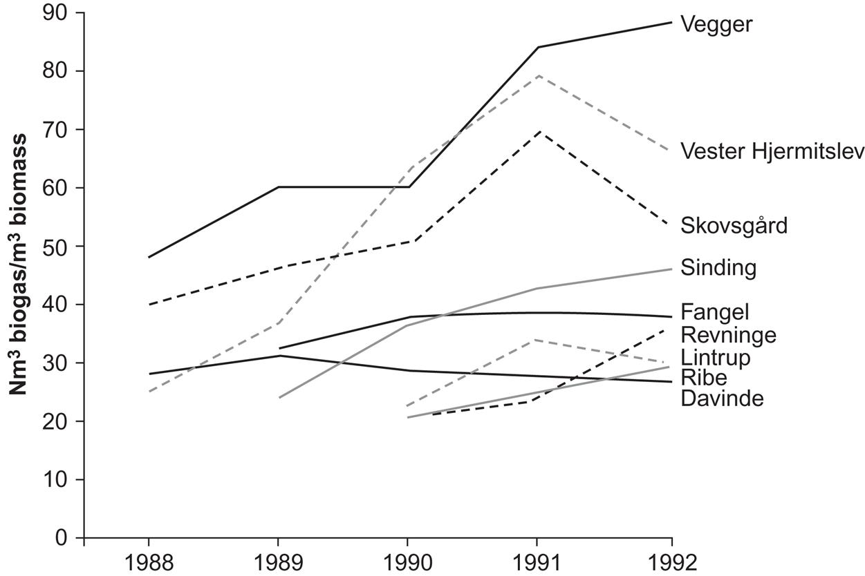
Some city sewage plants produce biogas (by anaerobic fermentation of the sewage) as one step in the cleaning procedure, using the biogas as fuel for driving mechanical cleaning devices, etc. Thus, in many cases, it is possible to avoid the need for other energy inputs and, in some cases, the plant becomes a net energy producer (Danish Energy Agency, 1992). Figure 4.121 shows the system layout for a biogas plant processing 300 t of biomass per day and accepting multiple types of feedstock; the plant is capable of delivering power, process and district heat, and fertilizer. Figure 4.122 gives the measured performance data for nine large prototype biogas plants in Denmark.
Because of the many complex processes involved in fermentation, yields vary in ways that are not always fully understood. Recent studies have indicated that microbial contamination is an important reason for reducing efficiency. Use of sterilization or antibiotics is not only expensive but may produce resistance. A better solution would be to improve the competitive advantage of the desired microbes over the undesired ones. Doing so by genetic engineering has been demonstrated in specific cases by Shaw et al. (2016).
4.6.3 Energy balance
The 1992 average production from large Danish biogas plants was 35.1 m3 per m3 of biomass (at standard pressure, methane content in the biogas being on average 64%), or 806 MJ m−3 (Tafdrup, 1993). In-plant energy use amounted to 90 MJ m−3, distributed in 28 MJ of electricity and 50 MJ of heat, all produced by the biogas plant itself. Fuel used in transporting manure to the plant totaled 35 MJ, and the fertilizer value of the returned residue was estimated at 30 MJ. Thus, the net outside energy requirement was 5 MJ for a production of 716 MJ, or 0.7%, corresponding to an energy payback time of 3 days. If the in-plant biogas use is added, energy consumption in the process is 13%. The energy for construction of the plant, which has not been estimated, should also be added. However, the best plants roughly break even economically, indicating that the overall energy balance is acceptable.
4.6.4 Greenhouse gas emissions
Using, as in the energy balance section above, the average of large Danish plants as an example, the avoided CO2 emission from having combined power and heat production use biomass instead of coal as a fuel is 68 kg per m3 of biomass converted. Added should be emissions from transportation of biomass, estimated at 3 kg, and the avoided emissions from conventional production of fertilizer, which is replaced by biogas residue, estimated at 3 kg. Reduced methane emissions, relative to the case of spreading manure directly on fields, is of the order of 61 kg CO2 equivalent (Tafdrup, 1993). The nitrous oxide balance is possibly improved by reducing denitrification in the soil, but high uncertainty makes actual estimates difficult at the present. The overall CO2 reduction obtained by summing up the estimates given above is then 129 kg for each m3 of biomass converted to biogas.
4.6.5 Other environmental effects
Compared to the current mix of coal, oil, and natural gas plants, biogas plants have two to three times lower SO2 emission but a correspondingly higher NOx emission. Higher ammonia content in the digested residue calls for greater care in using fertilizer from biogas plants, in order to avoid loss of ammonia. This is also true regarding avoiding loss of nutrients from fertilizer to waterways. Compared to unrefined manure, biogas-residue fertilizer has a marked gain in quality, including a better-defined composition, which contributes to using the correct dosage and avoiding losses to the environment. The dissemination of biogas plants removes the need for landfills, which is an environmental improvement. Odor is moved from the fields (where manure and slurry would otherwise be spread) to the biogas plant, where it can be controlled by suitable measures, such as filters (Tafdrup, 1993).
4.6.6 Hydrogen-producing cultures
Biochemical routes to fuel production include a number of schemes not presently developed to a technical or economic level of commercial interest. Hydrogen is a fuel that may be produced directly by biological systems. Hydrogen enters in photosynthesis in green plants, where the net result of the process is
However, the electrons and protons do not combine directly to form hydrogen,
but instead transfer their energy to a more complex molecule (NADPH2; cf. Chapter 3), which can drive the CO2 assimilation process. By this mechanism, plants avoid recombination of oxygen and hydrogen from the two processes mentioned above. Membrane systems keep the would-be reactants apart, and thus the energy-rich compound may be transported to other areas of the plant, where it takes part in plant growth and respiration.
Much thought has been given to modifications of plant material (e.g., by genetic engineering) in such a way that free hydrogen is produced on one side of a membrane and free oxygen on the other side (Berezin and Varfolomeev, 1976; Calvin, 1974; Hall et al., 1979).
While dissociation of water (by light) into hydrogen and oxygen (photolysis; cf. Chapter 5) does not require a biological system, it is possible that utilization of the process on a realistic scale can be more easily achieved if the critical components of the system, notably the membrane and the electron transport system, are of biological origin. Still, much more research is required before any thought can be given to practical application of direct biological hydrogen production cultures.
4.6.6.1 Thermochemical gasification of biomass
Conversion of fossil biomass, such as coal, into a gas is considered a way of reducing the negative environmental effects of coal utilization. However, in some cases, the effects have only been moved, not eliminated. Consider, for example, a coal-fired power plant with 99% particle removal from flue gases. If it were to be replaced by a synthetic gas-fired power plant with gas produced from coal, then sulfur could be removed at the gasification plant using dolomite-based scrubbers. This would practically eliminate the sulfur oxide emissions, but, on the other hand, dust emissions from the dolomite processing would represent particle emissions twice as large as those avoided at the power plant by using gas instead of coal (Pigford, 1974). Of course, the dust is emitted at a different location.
This example, as well as the health effects of both surface and underground coal mining (and the effects are not identical), has sparked interest in methods of gasifying coal in situ. Two or more holes are drilled. Oxygen (or air) is injected through one, and a mixture of gases, including hydrogen and carbon oxides, emerges at the other hole. The establishment of proper communication between holes, and suitable underground contact surfaces, has proved difficult, and recovery rates are modest.
The processes involved include
(4.158)
(4.159)
The stoichiometric relation between CO and H2 can then be adjusted using the shift reaction (4.159), which may proceed in both directions, depending on steam temperature and catalysts. This opens the way for methane synthesis through the reaction
(4.160)
At present, the emphasis is on improving gasifiers using coal already extracted. Traditional methods include the Lurgi fixed-bed gasifier (providing gas under pressure from non-caking coal at a conversion efficiency as low as 55%) and the Koppers–Totzek gasifier (oxygen input, the produced gas unpressurized, also of low efficiency).
Improved process schemes include the hy-gas process, requiring a hydrogen input; the bi-gas concept of brute force gasification at extremely high temperatures; and the slagging Lurgi process, capable of handling powdered coal (Hammond, 1976).
Promising, but still at an early stage of development, is catalytic gasification (e.g., using a potassium catalyst), where all processes take place at one relatively low temperature, so that they can be combined in a single reactor (Fig. 4.123). The primary reaction here is
(4.161)

(H2O being in the form of steam above 550°C), to be followed by (4.156) and (4.160). The catalyst allows all processes to take place at 700°C. Without a catalyst, the gasification would have to take place at 925°C and the shift reaction and methanation at 425°C, that is, in a separate reactor where excess hydrogen or carbon monoxide would be lost (Hirsch et al., 1982).
In a coal gasification scheme, storage would be (of coal) before conversion. Peat can be gasified in much the same way as coal, as can wood (with optional subsequent methanol conversion, as described in section 4.8.3).
4.6.7 Fresh biomass gasification
Gasification of biomass, and particularly wood and other lignin-containing cellulosic material, has a long history. The processes may be viewed as “combustion-like” conversion, but with less oxygen available than needed for burning. The ratio of oxygen available and the amount of oxygen that would allow complete burning is called the equivalence ratio. For equivalence ratios below 0.1, the process is called pyrolysis, and only a modest fraction of the biomass energy is found in the gaseous product—the rest being in char and oily residues. If the equivalence ratio is between 0.2 and 0.4, the process is called a proper gasification. This is the region of maximum energy transfer to the gas (Desrosiers, 1981).
The chemical processes involved in biomass gasification are similar to reactions (4.158)–(4.161) for coal gasification. Table 4.6 lists a number of reactions involving polysaccharidic material, including pyrolysis and gasification. In addition to the chemical reaction formulae, the table gives enthalpy changes for idealized reactions (i.e., neglecting the heat required to bring the reactants to the appropriate reaction temperature).
Table 4.6
Energy change for idealized cellulose thermal conversion reactions
| Chemical Reaction | Energy Consumed (kJ g−1)a | Products/Process |
| C6H10O5→6C+5H2+2.5O2 | 5.94b | Elements, dissociation |
| C6H10O5→6C+5H2O(g) | −2.86 | Charcoal, charring |
| C6H10O5→0.8C6H8O+1.8H2O(g)+1.2CO2 | −2.07c | Oily residues, pyrolysis |
| C6H10O5→2C2H4+2CO2+H2O(g) | 0.16 | Ethylene, fast pyrolysis |
| C6H10O5+‰O2→6CO+5H2 | 1.85 | Synthesis gas, gasification |
| C6H10O5+6H2→6″CH2″+5H2O(g) | −4.86d | Hydrocarbons, –generation |
| C6H10O5+6O2→6CO2+5H2O(g) | −17.48 | Heat, combustion |
aSpecific reaction heat.
bThe negative of the conventional heat of formation calculated for cellulose from the heat of combustion of starch.
cCalculated from the data for the idealized pyrolysis oil C6H8O (ΔHc=−745.9 kcal mol−1, ΔHf=149.6 kcal g−1, where Hc=heat of combustion and Hf=heat of fusion).
dCalculated for an idealized hydrocarbon with ΔHc as above. H2 is consumed.
Source: T. Reed (1981), in Biomass gasification (T. Reed, Ed.), reproduced with permission. Copyright 1981, Noyes Data Corporation, Park Ridge, NJ.
Figure 4.124 gives the energy of the final products, gas and char, as a function of the equivalence ratio, still based on an idealized thermodynamic calculation. The specific heat of the material is 3 kJ g−1 of wood at the peak of energy in the gas, increasing to 21 kJ g−1 of wood for combustion at equivalence ratio equal to unity. Much of this sensible heat can be recovered from the gas, so that process heat inputs for gasification can be kept low.

Figure 4.125 gives the equilibrium composition calculated as a function of the equivalence ratio. Equilibrium composition is defined as the composition of reaction products occurring after the reaction rates and reaction temperature have stabilized adiabatically. The actual processes are not necessarily adiabatic; in particular, the low-temperature pyrolysis reactions are not. Still, the theoretical evaluations assuming equilibrium conditions serve as a useful guideline for evaluating the performance of actual gasifiers.

The idealized energy change calculation of Table 4.6 assumes a cellulosic composition like the one in (4.153). For wood, the average ratios of carbon, hydrogen, and oxygen are 1:1.4:0.6 (Reed, 1981).
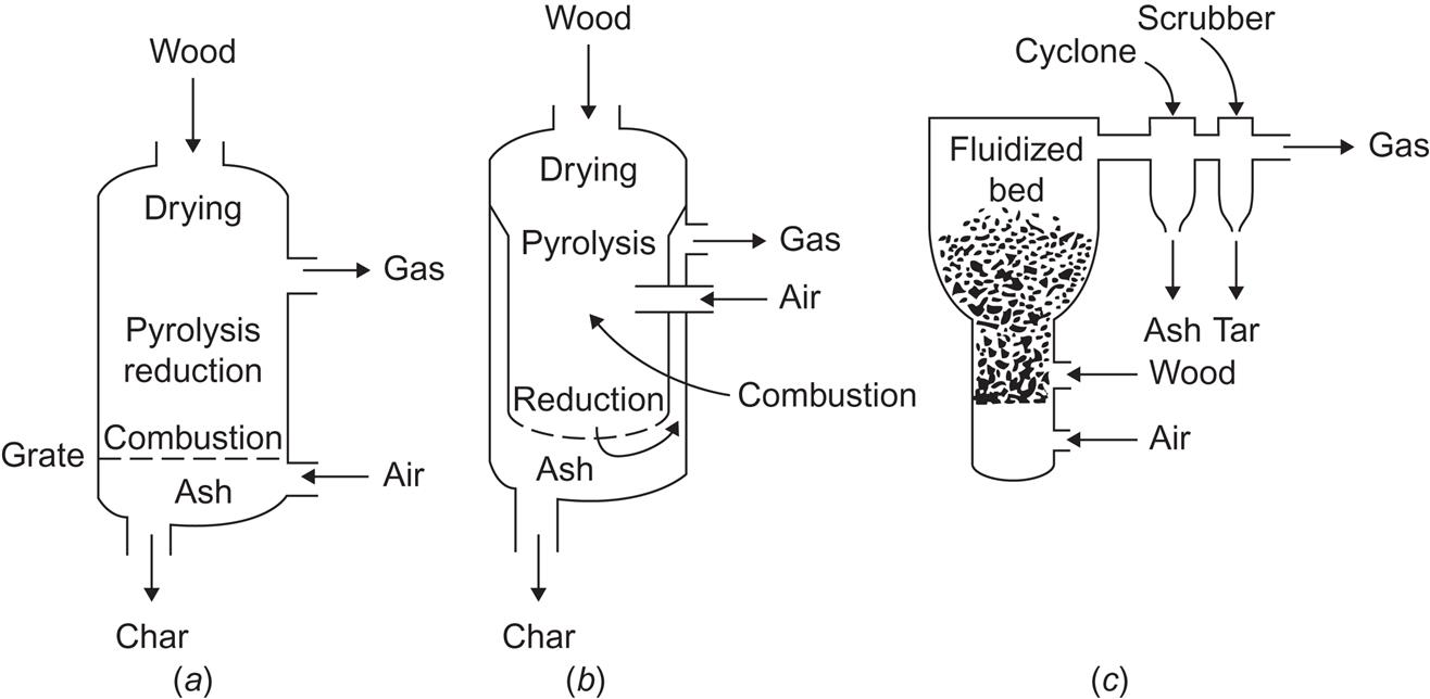
Figure 4.126 shows three examples of wood-gasifiers: the updraft, the downdraft, and the fluidized-bed types. The drawback of the updraft type is a high rate of oil, tar, and corrosive chemical formation in the pyrolysis zone. This problem is solved by the downdraft version, where oils and other matter pass through a hot charcoal bed in the lower zone of the reactor and become simpler gases or char. The fluidized-bed reactor may prove superior for large-scale operations, because its passage time is smaller. Its drawback is that ash and tars are carried along with the gas and have to be removed later in cyclones and scrubbers. Several variations on these gasifier types have been suggested (Drift, 2002; Gøbel et al., 2002).
The gas produced by gasification of biomass is a “medium-quality” gas; meaning a gas with burning value in the range 10–18 MJ m−3. This gas may be used directly in Otto or diesel engines, it may be used to drive heat pump compressors, or alternatively, it may be upgraded to pipeline-quality gas (about 30 MJ m−3) or converted to methanol, as discussed in section 4.6.3.
Environmental impacts of biomass gasifiers derive from biomass production, collection (e.g., forestry work), and transport to the gasification site, from the gasification and related processes, and finally from the use made of the gas. The gasification residues—ash, char, liquid wastewater, and tar—have to be disposed of. Char may be recycled to the gasifier, while ash and tars could conceivably be utilized in road building or the construction industry. The alternative, landfill disposal, is a recognized impact. Investigations of emissions from combustion of producer gas find lower emissions of nitrous oxides and hydrocarbons than in combustion of natural gas. In one case, carbon monoxide emissions were found to be higher than for natural gas burning, but it is believed that this can be rectified as more experience in adjusting air-to-fuel ratios is gained (Wang et al., 1982).
4.6.8 Biological conversion into liquid biofuels
Anaerobic fermentation processes may also be used to produce liquid fuels from biological raw materials. An example is ethanol production (4.152) from glucose, known as standard yeast fermentation in the beer, wine, and liquor industries. It has to take place in steps, so that the ethanol is removed (by distillation or dehydrator application) whenever its concentration approaches a value (around 12%) that would impede reproduction of the yeast culture.
To reduce the primary biological material (e.g., molasses, cellulose pulp, or citrus fruit wastes) to glucose, hydrolysis (4.157) may be used. Some decomposition takes place in any acid solution, but in order to obtain complete hydrolysis, specific enzymes must usually be provided, either directly or by adding microorganisms capable of forming such enzymes. The yeast themselves contain enzymes capable of decomposing polysaccharides into glucose. The theoretical maximum efficiency of glucose-to-ethanol conversion (described in more detail below) is 97%. According to Calvin (1977), in 1974 the Brazilian alcohol industry obtained 14% of the energy in raw sugar input in the form of ethanol, which was produced by fermentation of just the molasses residues from sugar refining, i.e., in addition to the crystallized sugar produced. Currently, the figure is 25% of input sugar energy (see Fig. 4.128) for an optimized plant design (EC, 1994). The sustainability of the Brazilian use of bioethanol from sugarcane as a 20% blend into gasoline has been discussed by Goldemberg et al. (2007).

Mechanical energy inputs, e.g., for stirring, could be covered by burning the fermentation wastes in a steam power plant. In the European example illustrated in Fig. 4.128, such inputs amount to about a third of the energy inputs through the sugar itself.
Fermentation processes based on molasses or other sugar-containing materials produce acetone–butanol, acetone–ethanol, or butanol–isopropanol mixtures when the proper bacteria are added. In addition, carbon dioxide and small amounts of hydrogen are formed (see, for example, Beesch, 1952; Keenan, 1977).
Conversion of fossilized biomass into liquid fuels is briefly mentioned at the beginning of section 4.6.2, in conjunction with Fig. 4.111, which shows an overview of the conversion routes open for biofuel generation. Among the non-food energy uses of biomass, there are several options leading to liquid fuels that may serve as a substitute for oil products. The survey of conversion processes given in Fig. 4.111 indicates liquid end-products as the result of either biochemical conversion using fermentation bacteria or a thermochemical conversion process involving gasification and, for example, further methanol synthesis. The processes that convert biomass into liquid fuels that are easy to store are discussed below, but first the possibility of direct production of liquid fuels by photosynthesis is presented.
4.6.8.1 Direct photosynthetic production of hydrocarbons
Oil from the seeds of many plants, such as rape, olive, groundnut, corn, palm, soybean, and sunflower, is used as food or in the preparation of food. Many of these oils will burn readily in diesel engines and can be used directly or mixed with diesel oil of fossil origin, as they are indeed in several pilot projects around the world. However, for most of these plants, oil does not constitute a major fraction of the total harvest yield, and use of these crops to provide oil for fuel use could interfere with food production. A possible exception is palm oil, because intercropping of palm trees with other food crops may prove advantageous, by retaining moisture and reducing wind erosion.
Therefore, interest is concentrated on plants that yield hydrocarbons and that, at the same time, are capable of growing on land unsuited for food crops. Calvin (1977) first identified the Euphorbia plant genus as a possibility. The rubber tree, Hevea brasiliensis, is in this family, and its rubber is a hydrocarbon–water emulsion, the hydrocarbon of which (polyisoprenes) has a large molecular weight, about a million, making it an elastomer. However, other plants of the genus Euphorbia yield latex of much lower molecular weight which could be refined in much the same way as crude oil. In the tropical rainforests of Brazil, Calvin found a tree, Copaifera langsdorffii, which annually yields some 30 liters of virtually pure diesel fuel (Maugh, 1979). Still, interest centers on species that are likely to grow in arid areas like the deserts of the southern United States, Mexico, Australia, and so on.
Possibilities include Euphorbia lathyris (gopher plant), Simmondsia chinensis (jojoba), Cucurbita foetidissima (buffalo gourd), and Parthenium argentatum (guayule). The gopher plant has about 50% sterols (on a dry weight basis) in its latex, 3% polyisoprene (rubber), and a number of terpenes. The sterols are suited as feedstocks for replacing petroleum in chemical applications. Yields of first-generation plantation experiments in California are 15–25 barrels of crude oil equivalent or some 144 GJ ha−1 (i.e., per 104 m2). In the case of Hevea, genetic and agronomic optimization has increased yields by a factor of 2000 relative to those of wild plants, so high hydrocarbon production rates should be achievable after proper development (Calvin, 1977; Johnson and Hinman, 1980; Tideman and Hawker, 1981). Other researchers are less optimistic (Stewart et al., 1982; Ward, 1982).
4.6.8.2 Alcohol fermentation
The ability of yeast and bacteria like Zymomonas mobilis to ferment sugar-containing material to form alcohol is well known from beer, wine, and liquor manufacture. If the initial material is cane sugar, the fermentation reaction may be summarized as
(4.162)
The energy content of ethanol is 30 MJ kg−1, and its octane rating is 89–100. With alternative fermentation bacteria, the sugar may be converted into butanol, C2H5(CH2)2OH. In Brazil, the cost of ethanol has finally been lowered to equal that of gasoline (Johansson, 2002).
In most sugar-containing plant material, the glucose molecules exist in polymerized form, such as starch or cellulose, of the general structure (C6H10O5)n. Starch or hemicellulose is degraded to glucose by hydrolysis (cf. Fig. 4.111), while lignocellulose resists degradation owing to its lignin content. Lignin glues the cellulosic material together to keep its structure rigid, whether it be crystalline or amorphous. Wood has a high lignin content (about 25%), and straw also has considerable amounts of lignin (13%), while potato and beet starch contain very little lignin.
Some of the lignin seals may be broken by pretreatment, ranging from mechanical crushing to the introduction of swelling agents causing rupture (Ladisch et al., 1979).
The hydrolysis process is given by (4.153). In earlier times, hydrolysis was always achieved by adding an acid to the cellulosic material. During both world wars, Germany produced ethanol from cellulosic material by acid hydrolysis, but at very high cost. Acid recycling is incomplete; with low acid concentration, the lignocellulose is not degraded, and, with high acid concentration, the sugar already formed from hemicellulose is destroyed.
Consequently, alternative methods of hydrolysis have been developed, based on enzymatic intervention. Bacteria (e.g., of the genus Trichoderma) and fungi (such as Sporotrichum pulverulentum) have enzymes that have proved capable of converting cellulosic material, at near ambient temperatures, to some 80% glucose and a remainder of cellodextrins (which could eventually be fermented, but in a separate step with fermentation microorganisms other than those responsible for the glucose fermentation) (Ladisch et al., 1979).
The residue left behind after the fermentation process (4.162) can be washed and dried to give a solid product suitable as fertilizer or as animal feed. The composition depends on the original material, in particular with respect to lignin content (small for residues of molasses, beets, etc., high for straws and woody material, but with fiber structure broken as a result of the processes described above). If the lignin content is high, direct combustion of the residue is feasible, and it is often used to furnish process heat to the final distillation.
The outcome of the fermentation process is a water–ethanol mixture. When the alcohol fraction exceeds about 10%, the fermentation process slows down and finally halts. Therefore, an essential step in obtaining fuel alcohol is to separate the ethanol from the water. Usually, this is done by distillation, a step that may make the overall energy balance of ethanol production negative. The sum of agricultural energy inputs (fertilizer, vehicles, machinery) and all process inputs (cutting, crushing, pretreatment, enzyme recycling, heating for different process steps from hydrolysis to distillation), as well as energy for transport, is, in existing operations, such as those of the Brazilian alcohol program (Trinidade, 1980), around 1.5 times the energy outputs (alcohol and fertilizer if it is utilized). However, if the inputs are domestic fuels, for example, combustion of residues from agriculture, and if the alcohol produced is used to displace imported oil products, the balance might still be quite acceptable from a national economic point of view.
If, further, the lignin-containing materials of the process are recovered and used for process heat generation (e.g., for distillation), then such energy should be counted not only as input but also as output, making the total input and output energy roughly balance. Furthermore, more sophisticated process design, with cascading heat usage and parallel distillation columns operating with a time displacement such that heat can be reused from column to column (Hartline, 1979), could reduce the overall energy inputs to 55–65% of the outputs.
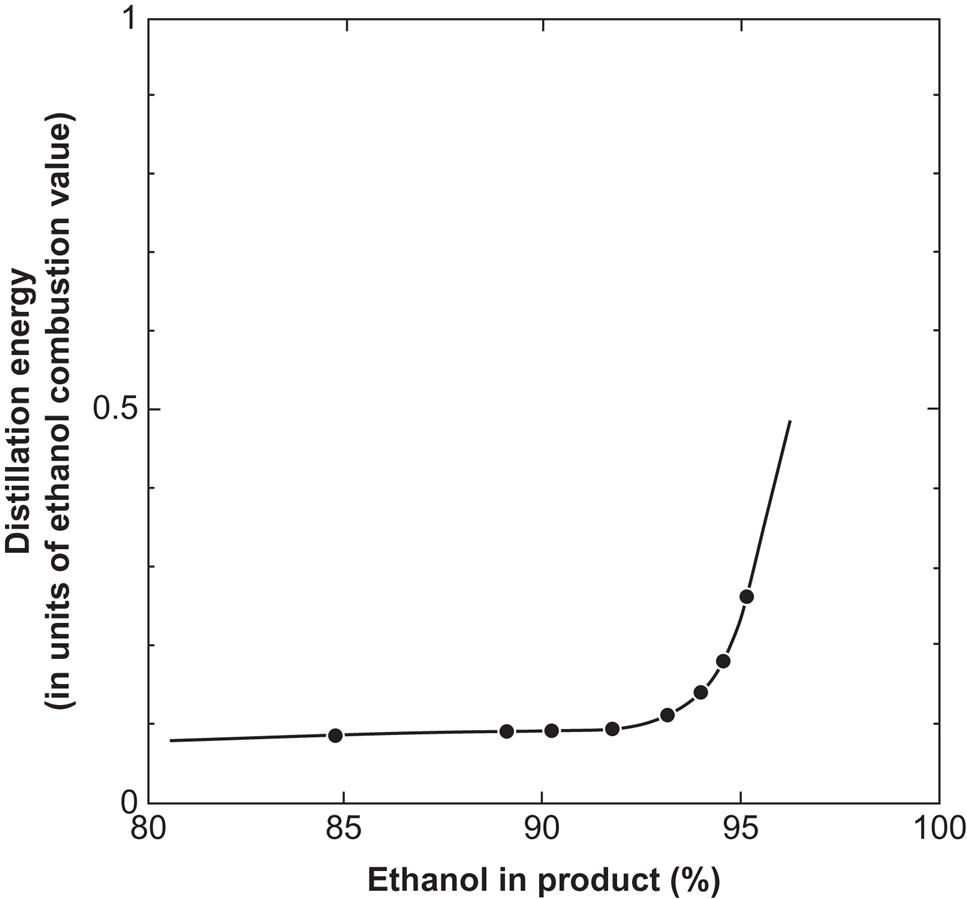
Energy balances would be radically improved if distillation could be replaced by a less energy-intensive separation method. Several such methods for separating water and ethanol have been demonstrated on a laboratory scale, including drying with desiccants, such as calcium hydroxide, cellulose, or starch (Ladisch and Dyck, 1979); gas chromatography using rayon to retard water, while organic vapors pass through; solvent extraction using dibutyl phthalate, a water-immiscible solvent of alcohols; and passage through semipermeable membranes or selective zeolite absorbers (Hartline, 1979) and phase separation (APACE, 1982). The use of dry cellulose or starch appears particularly attractive, because over 99% pure alcohol can be obtained with less than 10% energy input, relative to the combustion energy of the alcohol. Furthermore, the cellulosic material may be cost-free, if it can be taken from the input stream to the fermentation unit and returned to it after having absorbed water (the fermentation reaction being “wet” anyway). The energy input of this scheme is for an initial distillation, bringing the ethanol fraction of the aqueous mixture from the initial 5–12% up to about 75%, at which point the desiccation process is started. As can be seen from Fig. 4.127, the distillation energy is modest up to an alcohol content of 90% and then starts to rise rapidly. The drying process thus substitutes for the most energy-expensive part of the distillation process.
Ethanol fuel can be stored and used in the transportation sector much the same way as gasoline is used. It can be mixed with gasoline or can fully replace gasoline in spark ignition engines with high compression ratios (around 11). The knock resistance and high octane number of ethanol make this possible, and with preheating of the alcohol (using combustion heat that is recycled), the conversion efficiency can be improved. Several countries presently use alcohol–gasoline blends with up to 10% ethanol, and these blends do not require any engine modification. Altering gasoline Otto engines may be inconvenient in a transition period, but if alcohol distribution networks are implemented and existing gas stations modified, then car engines could be optimized for alcohol fuels without regard to present requirements. A possible alternative to spark ignition engines is compression ignition engines, where auto-ignition of the fuel under high compression (a ratio of 25) replaces spark or glow plug ignition. With additives or chemical transformation into acetal, alcohol fuels could be used this way (Bandel, 1981). Ethanol does not blend with diesel oil, so mixtures require the use of special emulsifiers (Reeves et al., 1982). However, diesel oil can be mixed with other biofuels without problems, e.g., the plant oils (rapeseed oil, etc.) presently in use in Germany.
A number of concerns about the socioeconomic impacts of the ethanol fermentation energy conversion chain must be considered, in addition to the environmental impacts considered, e.g., by Goldemberg et al. (2007) mentioned above. First, the biomass being used may have direct uses as food or may be grown in competition with food production. The reason is, of course, that the easiest ethanol fermentation is obtained by starting with a raw material with the highest possible elementary sugar content, that is, starting with sugar cane or cereal grain. Since sugar cane is likely to occupy prime agricultural land, and cereal production must increase with increasing world population, neither of these biomass resources should be used as fermentation inputs. Food competing biofuel products are termed “first-generation biofuels”. However, residues from cereal production and from necessary sugar production (in many regions of the world, sugar consumption is too high from a health and nutrition point of view) could be used for ethanol fermentation, together with urban refuse, extra crops on otherwise committed land, perhaps aquatic crops, and forest renewable resources, termed “second-generation biofuels” (the impact difference between first- and second-generation biofuels is quantified by Fargione et al., 2008). The remarks made in Chapter 3 about proper soil management, recycling nutrients, and covering topsoil to prevent erosion also apply to the enhanced tillage utilization that characterizes combined food and ethanol production.
The hydrolysis process involves several potential environmental effects. If acids are used, corrosion and accidents may occur, and substantial amounts of water would be required to clean the residues for re-use. Most of the acid would be recovered, but some would follow the sewage stream. Enzymatic hydrolysis seems less risky. Most of the enzymes would be recycled, but some might escape with wastewater or residues. Efforts should be made to ensure that they are made inactive before release. This is particularly important when, as envisaged, the fermentation residues are to be brought back to the fields or used as animal feed. A positive impact is the reduction of pathogenic organisms in residues after fermentation.
Transport of biomass could involve dust emissions, and transport of ethanol might lead to spills (in insignificant amounts, as far as energy is concerned, but with possible local environmental effects), but, overall, the impact from transport would be very small.
Finally, the combustion of ethanol in engines or elsewhere leads to pollutant emissions. Compared with gasoline combustion, ethanol combustion in modified ignition engines has lower emissions of carbon monoxide and hydrocarbons, but increased emissions of nitrous oxides, aromatics, and aldehydes (Hespanhol, 1979). When special ethanol engines and exhaust controls are used, critical emissions may be controlled. In any case, the lead pollution from gasoline engines still ongoing in some countries would be eliminated.
The energy balance of current ethanol production from biomass is not very favorable. A European study has estimated the energy flows for a number of feedstocks (EC, 1994). The highest yield, about 100 GJ ha−1, is for sugar beets, shown in Fig. 4.128, but the process energy inputs and allotted life-cycle inputs into technical equipment are as large as the energy of the ethanol produced. A part of the process energy may be supplied by biogas co-produced with the ethanol, but the overall energy efficiency remains low.
In a life-cycle analysis of ethanol production (cf. Chapter 7), the fact that such production is currently based upon energy crops rather than on residues (sugar cane or beets, rather than straw and husk) means that all energy inputs and environmental effects from the entire agricultural feedstock production should be included, along with the effects pertaining to ethanol plants and downstream impact. Clearly, in this mode it is very difficult to balance energy outputs and inputs and to reach acceptable impact levels. Interest should therefore be limited to bioenergy processes involving only residues from an otherwise sensible production (food or wood). Among these second-generation technologies, bioethanol is a prominent possibility (Tan et al., 2008).
4.6.8.3 Methanol from biomass
There are various ways of producing methanol from biomass sources, as indicated in Fig. 4.111. Starting from wood or isolated lignin, the most direct routes are liquefaction and gasification. Pyrolysis gives only a fraction of energy in the form of a producer gas.
High-pressure hydrogenation transforms biomass into a mixture of liquid hydrocarbons suitable for further refining or synthesis of methanol (Chartier and Meriaux, 1980), but all methanol production schemes so far have used a synthesis gas, which may be derived from wood gasification or coal gasification. The low-quality “producer gas” resulting directly from wood gasification (used, as mentioned, in cars throughout Europe during World War II) is a mixture of carbon monoxide, hydrogen gas, carbon dioxide, and nitrogen gas (see section 4.6.2). If air is used for gasification, the energy conversion efficiency is about 50%, and if pure oxygen is used instead, some 60% efficiency is possible and the gas produced has a lower nitrogen content (Robinson, 1980). Gasification or pyrolysis could conceivably be performed with heat from (concentrating) solar collectors, for example, in a fluidized-bed gasifier maintained at 500°C.
The producer gas is cleaned, CO2 and N2 as well as impurities are removed (the nitrogen by cryogenic separation), and methanol is generated at elevated pressure by the reaction
(4.163)
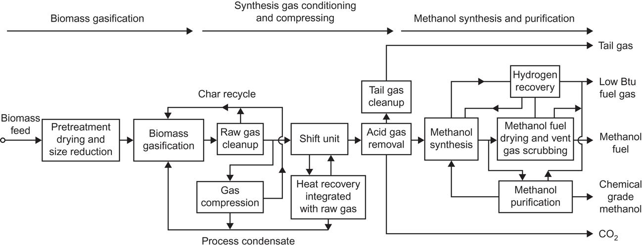
The carbon monoxide and hydrogen gas (possibly with additional CO2) is called the synthesis gas, and it is usually necessary to use a catalyst in order to maintain the proper stoichiometric ratio between the reactants of (4.163) (Cheremisinoff et al., 1980). A schematic process diagram is shown in Fig. 4.129.
An alternative is biogas production from the biomass (section 4.6.2) followed by the methane to methanol reaction,
(4.164)
also used in current methanol production from natural gas (Wise, 1981). Change of the H2/CO stoichiometric ratio for (4.163) is obtained by the shift reaction (4.159) discussed in section 4.6.2. Steam is added or removed in the presence of a catalyst (iron oxide, chromium oxide).
The conversion efficiency of the synthesis-gas-to-methanol step is about 85%, implying an overall wood to methanol energy efficiency of 40–45%. Improved catalytic gasification techniques raise the overall conversion efficiency to about 55% (Faaij and Hamelinck, 2002). The efficiency currently achieved is about 50%, but not all life-cycle estimates of energy inputs have been included or performed (EC, 1994).
The octane number of methanol is similar to that of ethanol, but the heat of combustion is less, amounting to 18 MJ kg−1. However, the engine efficiency of methanol is higher than that of gasoline, by at least 20% for current automobile car engines, so an “effective energy content” of 22.5 MJ kg−1 is sometimes quoted (EC, 1994). Methanol can be mixed with gasoline in standard engines, or used in specially designed Otto or diesel engines, such as a spark ignition engine run on vaporized methanol, with the vaporization energy being recovered from the coolant flow (Perrin, 1981). The uses of methanol are similar to those of ethanol, but there are several differences in the environmental impact from production to use (e.g., toxicity of fumes at filling stations).
The future cost of methanol fuel is expected to reach US$ 8/GJ (Faaij and Hamelinck, 2002). The gasification can be done in closed environments, where all emissions are collected, as well as ash and slurry. Cleaning processes in the methanol formation steps will recover most catalysts in re-usable form, but other impurities would have to be disposed of, along with the gasification products. Precise schemes for waste disposal have not been formulated, but it seems unlikely that all nutrients could be recycled to agri- or silviculture, as in the case for ethanol fermentation (SMAB, 1978). However, production of ammonia by a process similar to the one yielding methanol is an alternative use of the synthesis gas. Production of methanol from Eucalyptus rather than from woody biomass has been studied in Brazil (Damen et al., 2002). More fundamental research, aimed at a better understanding of how methanol production relies on degradation of lignin, is ongoing (Minami et al., 2002). On the usage side, direct transformation of methane into a transportable, liquid fuel has been investigated (Morejudo et al., 2016).
4.6.9 Enzymatic decomposition of cellulosic material
Sustainable use of biomass for fuels requires CO2 neutrality and recycling of nutrients, as well as recognition of the use of biomass for other purposes, such as food production, construction materials, and other uses (e.g., fiber for materials). The different uses of biomass in society must be balanced, and meeting the food requirements of the world’s large human population naturally has first priority.
The difference between edible and non-edible biomass is largely that the edible parts (cereals, fruits, etc.) contain amylose (starch) or fructose and the non-edible parts have a strong component of cellulose (which can be used as fiber for clothes and other materials or in construction materials). As illustrated in Fig. 4.130, amylose is made from repeating glucose segments, while in cellulose, each second glucose-molecule segment is turned 180°. This “small” difference makes cellulose fibers very strong, while starch pieces are curling, separating, fragile, and, first of all, digestible.

Agricultural and forestry residues, usually straw or woodchips plus some wet components, are mostly composed of cellulose (long β-(1,4)-glucan polymers), hemicellulose (short, branched polymers of sugars), and lignin (polymers derived from coumaryl, coniferyl and sinapyl alcohol). Transformation of these components to transportation fuels uses a variety of methods that exhibit different efficiencies for the three types of components. Selecting the best method for breaking down cellulosic material requires understanding of the genomics of the material (Rubin, 2008) and it has been suggested that genetic modification of the primary plants could result in more amenable starting points for biofuel synthesis (Ragauskas et al., 2006).
In contrast to starch sugar crops, such as cereal grains, currently used by the biofuel industry (chiefly in Brazil and the United States), which can be transformed into ethanol by fermentation, and the oil-containing plant parts (e.g., rapeseed) that can be transformed into biodiesel fuel by transesterification (mainly in Europe and the United States; Korbitz, 1999; Huang et al., 2010, starting from microalgae), lignin and cellulosic polymers require more elaborate processes. As mentioned, the starch- and oil-based fuels are called first-generation biofuels and they are in competition with food production. Those that are not in such competition are called second-generation biofuels (Naik et al., 2010).
The second-generation biofuel processes currently receiving most attention entail: first, mechanical or chemical pretreatment to break down the fiber structure of the biomass feedstock, allowing hydrolytic transformation of cellulose or lignin into simple sugars; and, subsequently, a fermentation process to arrive at the biofuel. Hydrolysis is basically the splitting of water into H+ ions and OH− ions, but, in a biomass context, it describes the transformation of polysaccharide chains like those shown in Fig. 4.130 into simple soluble sugars. Hydrolysis can be monitored in real time by measuring heat flows associated with it (Murphy et al., 2010).
There are several alternative routes from biomass to biofuels, such as high-temperature processes employing pyrolysis of the biomass into bio-oil, liquefaction into heavy oil, or the Fischer-Tropsch syngas route (with the shift reactions mentioned above after gasification in order to produce hydrogen or, further, hydrocarbons). Biological fermentation into methane also may be used to arrive at ethanol as an end-product, using suitable enzymes, and chemical reactions other than those involved in hydrolysis can be used (Perego and Bianchi, 2010). At present, all of these alternatives have conversion efficiencies below 50%.
Pretreatment may include mechanical crushing, acid treatment, and various catalytic processes. Pretreatment processes are required to allow operation at modest temperatures (200°C or lower) and to reach decent efficiencies (Öhgren et al., 2007; Yeh et al., 2010; Perego and Bianchi, 2010), but care should be taken in recovering the acids and catalysts used, because otherwise largescale production is not environmentally acceptable (Abbasi and Abbasi, 2010).
Different saccharification enzymes have been tried, most of them cellulases, which are complex mixtures of cellulose-degrading agents. However, the enzymatic processes still require that pretreatment has taken place to open the fiber structure and separate lignin from the celluloses (alkali processes, weak or strong acid processes, and steam explosion have been tried; see Perego and Bianchi, 2010). Pretreatment is the step that contributes most to making second-generation biofuels more expensive to produce than first-generation biofuels.