In horizontal decomposition, the dividing lines in the decomposition are between rows (so to speak) instead of between columns. The basic motivation for such decomposition is this: We shouldn’t try to use the same table to represent two or more different predicates. For example, consider table SC again as shown in either Figure C-2 or Figure C-3. In that table, the row for supplier S1 means: Supplier S1 is located in London. By contrast, the row for supplier S2 means: We don’t know where supplier S2 is located (at any rate, let’s agree that’s what it means for the time being). So different rows correspond to different predicates, and the predicate I gave for SC earlier—Supplier SNO is located in city CITY—doesn’t in fact apply to every row.

Now, we might try a different predicate, perhaps like this (note the OR, which I’ve shown in uppercase bold for emphasis):

But this predicate doesn’t work either. If we try to instantiate it with values (or “values,” rather) from the row for supplier S2, we get:

And the first half of this sentence—Supplier S2 is located in city ░ —still makes no sense, because ░ isn’t a legitimate city name and can’t legitimately be substituted as an argument for the CITY parameter in the putative predicate. So what we need to do is break the predicate into two separate pieces, as it were (more precisely, we need to break the two disjuncts apart); that is, we need to apply horizontal decomposition to table SC, to obtain one table for each of those disjuncts. The result of this step is the tables shown in Figure C-4:

Figure C-4. Horizontally decomposing table SC

As you can see, we now have two tables: (a) an abbreviated version of table SC (for which I’ve retained the name SC, for convenience), containing just the original SC rows that had no shaded entries in column CITY; and (b) another table SUC (suppliers with an unknown city), containing just the original SC rows that did have shaded entries in column CITY—except that the CITY column in that table, if we kept it, would contain nothing but shaded entries, and so we can discard it without losing any information. The predicates for these tables are as follows:

Observe in particular that the predicate for (this revised version of) table SC has two parameters, SNO and CITY, and that table has two columns accordingly; by contrast, the predicate for table SUC has just one parameter, SNO, and that table has just one column accordingly.

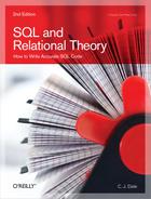
Of course, we can and should perform an analogous horizontal decomposition on table ST from Figure C-2. The result is shown in Figure C-5:

Figure C-5. Horizontally decomposing table ST

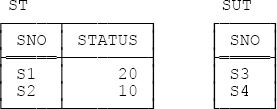
The predicates for the tables in Figure C-5 are as follows: