
Consider the following edited extract from Exercise 5.16 in Chapter 5:
The well known bill of materials application involves a relvar—PP, say—showing which parts contain which parts as immediate components. Of course, immediate components are themselves parts, and they can have further immediate components of their own.
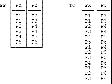
Figure 7-5 below shows (a) a sample value for that relvar PP and (b) the corresponding transitive closure TC.[108] The predicates are as follows:
PP: Part PX contains part PY as an immediate component.
TC: Part PX contains part PY as a component at some level (not necessarily immediate).
Given a (relation) value pp for relvar PP, the relation tc that’s the transitive closure of pp can be defined as follows:
Definition: The pair (px,py) appears in tc if and only if:
It appears in pp, or
There exists some pz such that the pair (px,pz) appears in pp and the pair (pz,py) appears in tc.
In other words, if we think of pp as representing a directed graph, with a node for each part and an arc from each node to each corresponding immediate component node, then (px,py) appears in the transitive closure if and only if there’s a path in that graph from node px to node py. Observe that the definition involves a recursive reference to relation tc.
Aside: In practice relvar PP would probably have a QTY attribute as well (showing how many instances of the immediate component part PY are needed to make one instance of part PX), and we would probably want to compute, not just the transitive closure as such, but also the total number of instances of part PY needed to make one instance of part PX: the gross requirements problem. I ignore this refinement for simplicity. End of aside.
It’s also possible to define the transitive closure procedurally (and iteratively):
     TC := PP ;
     do until TC reaches a "fixpoint" ;
        WITH ( R1 := PP RENAME { PY AS PZ } ,
               R2 := TC RENAME { PX AS PZ } ,
               R3 := ( R1 JOIN R2 ) { PX , PY } ) :
        TC := TC UNION R3 ;
     end ;
Loosely speaking, this code works by repeatedly forming an intermediate result consisting of the union of (a) the previous intermediate result and (b) a relation computed on the current iteration. The process is repeated until that intermediate result reaches a fixpoint (i.e., until it ceases to grow). Note: It’s easy to see the code is very inefficient!—in effect, each iteration repeats the entire computation of the previous one. In fact, it’s little more than a direct implementation of the original (recursive) definition. However, it could clearly be made more efficient if desired. Similar remarks apply to all of the code samples in the present section.
Turning now to Tutorial D, we could define a recursive operator (TCLOSE) to compute the transitive closure as follows:[109]
     OPERATOR TCLOSE ( XY RELATION { X ... , Y ... } )
                  RETURNS RELATION { X ... , Y ... } ;
        RETURN ( WITH ( R1 := XY RENAME { Y AS Z } ,
                        R2 := XY RENAME { X AS Z } ,
                        R3 := ( R1 JOIN R2 ) { X , Y } ,
                        R4 := XY UNION R3 ) :
                 IF R4 = XY THEN R4     /* unwind recursion */
                    ELSE TCLOSE ( R4 )  /* recursive invocation */
                 END IF ) ;
     END OPERATOR ;
Now, e.g., the expression TCLOSE(pp) will return the transitive closure of pp. Hence, for example, the expression
( TCLOSE ( PP ) WHERE PX = 'P1') { PY }will give the “bill of materials” for part P1, and the expression
( TCLOSE ( PP ) WHERE PY = 'P6') { PX }will give the “where used” list for part P6. Note: Computing the bill of materials for a given part is sometimes referred to as part explosion; likewise, computing the “where used” list for a given part is referred to as part implosion.
Now, SQL too supports what it calls “recursive queries.” Here’s an SQL expression to compute the transitive closure of PP:
     WITH RECURSIVE TC ( PX , PY ) AS
        ( SELECT PP.PX , PP.PY
          FROM   PP
          UNION  CORRESPONDING
          SELECT PP.PX , TC.PY
          FROM   PP , TC
          WHERE  PP.PY = TC.PX )
     SELECT PX , PY
     FROM   TC
As you can see, this expression too is a more or less direct transliteration of the original recursive definition.
Note: This book deliberately has very little to say about commercial SQL products. However, I’d like to offer a brief remark here regarding Oracle specifically. As you might know, Oracle has had some recursive query support for many years. By way of example, the query “Explode part P1” can be expressed in Oracle as follows:
     SELECT  LEVEL , PY
     FROM    PP
     CONNECT BY PX = PY
     START   WITH PX = 'P1'
I don’t want to explain in detail how this expression is evaluated—but I do want to show the result it produces, given the sample data of Figure 7-5. Here it is:
|
|
|
|
|
|
|
|
|
|
|
|
|
|
|
|
|
|
Note carefully that this result isn’t a relation (and the relational closure property has thereby been violated). First of all, it contains some duplicate rows; for example, the row (2,P4) appears twice. More important, those duplicate rows are not duplicate rows as we usually understand them in SQL (as they might appear in, say, the result of evaluating some SQL expression in the standard); that is, they aren’t just “saying the same thing twice,” as I put it in Chapter 4. To spell the point out, one of those two (2,P4) rows reflects the path in the graph from part P1 to part P4 via part P2; the other reflects the path in the graph from part P1 to part P4 via part P3. Thus, if we deleted one of those rows, we would lose information.
Aside: Actually the same kind of problem can arise in the SQL standard if the recursive query in question uses UNION ALL instead of UNION DISTINCT—as in practice such queries very typically do. Further details are beyond the scope of this book; however, if you try to code the gross requirements problem in SQL you might see for yourself why it’s tempting, at least superficially, to use UNION ALL. End of aside.
Note too that in addition to the foregoing violations, the ordering of the rows in the result is significant as well. For example, the reason we know the first (2,P4) row corresponds to the path from P1 to P4 via P2 specifically is because it immediately follows the row corresponding to the path from P1 to its immediate component P2. Thus, if we reordered the rows, again we would lose information.
Consider Figure 7-5 once again. Suppose the relation pp shown as a value for relvar PP in that figure additionally contained a tuple representing, say, the pair (P5,P1). Then there would be a cycle in the data (actually two cycles, one involving parts P1-P2-P4-P5-P1 and one involving parts P1-P3-P4-P5-P1). In the case of bill of materials, such cycles should presumably not be allowed to occur, since they make no sense. Sometimes, however, they do make sense; the classic example is a transportation network, in which there are routes from, say, New York (JFK) to London (LHR), London to Paris (CDG), and Paris back to New York again (as well as routes in all of the reverse directions, of course).
Now, the existence of a cycle in the data has no effect on the transitive closure as such. But it does have the potential to cause an infinite loop in certain kinds of processing. For example, a query to find travel routes from New York to Paris might—if we’re not careful—produce results as follows:
     JFK - LHR - CDG
     JFK - LHR - JFK - LHR - CDG
     JFK - LHR - JFK - LHR - JFK - LHR - CDG
     etc., etc. etc.
Of course, it might at least be possible to formulate the query in such a way as to exclude segments in which the destination city is JFK (since we certainly don’t want a route that takes us back to where we started). But even this trick will still allow routes such as:
JFK - ORD - LHR - ORD - LHR - ORD - LHR - ... - CDG
(ORD = Chicago). Moreover, it still won’t prevent an infinite loop. Now, we might prevent the infinite loop as such by rejecting routes involving, say, more than four segments; but under such a scheme we could still get, e.g., the route JFK-ORD-LHR-ORD-CDG. Clearly, what we need is a more general mechanism that will allow the query to recognize when a given node in the graph has been previously visited. And SQL does in fact include a feature, the CYCLE clause, that can be used in recursive queries to achieve such an effect. The specifics are a little complicated, and I don’t want to get into details here; suffice it to say that the CYCLE clause provides a means of tagging nodes (i.e., rows) as they’re visited, and then stopping the recursion if a tagged node is subsequently encountered again. For more details, I refer you to the standard document itself.
[108] Nothing to do with the closure property of the relational algebra.
[109] Actually Tutorial D goes beyond the relational algebra as conventionally understood in that it provides TCLOSE as a built in operator. I show it as a user defined operator here just to show how recursive operators can be defined in Tutorial D.