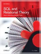
Recall from Chapter 2 that relations with relation valued attributes (RVAs for short) are legal. Figure 7-1 below shows relations R1 and R4 from Figure 2-1 and Figure 2-2 in that chapter; R4 has an RVA and R1 doesn’t, but the two relations clearly represent the same information.
Now, we obviously need a way to map between relations without RVAs and relations with them, and that’s the purpose of the GROUP and UNGROUP operators. I don’t want to go into a lot of detail on those operators here; let me just say that, given the relations shown in Figure 7-1, the expression
R1 GROUP ( { PNO } AS PNO_REL )will produce R4, and the expression
R4 UNGROUP ( PNO_REL )
By the way, it’s worth noting that the following expression—
EXTEND R1 { SNO } : { PNO_REL := !!R1 }—will produce exactly the same result as the GROUP example shown above. In other words, GROUP can be defined in terms of EXTEND and image relations. Now, I’m not suggesting that we get rid of our useful GROUP operator; quite apart from anything else, a language that had an explicit UNGROUP operator (as Tutorial D does) but no explicit GROUP operator could certainly be criticized on ergonomic grounds, if nothing else. But it’s at least interesting, and perhaps pedagogically helpful, to note that the semantics of GROUP can so easily be explained in terms of EXTEND and image relations.
And by the way again: If R4 includes exactly one tuple for supplier number Sx, say, and if the PNO_REL value in that tuple is empty, then the result of the foregoing UNGROUP will contain no tuple at all for supplier number Sx. For further details, I refer you to my book An Introduction to Database Systems (see Appendix G) or the book Databases, Types, and the Relational Model: The Third Manifesto (again, see Appendix G), by Hugh Darwen and myself.
The SQL counterparts to GROUP and UNGROUP are quite complex, and I don’t propose to go into details here. However, I will at least show SQL analogs of the Tutorial D examples above. Here first is the GROUP example:[106]
     SELECT DISTINCT X.SNO ,
                     TABLE ( ( SELECT Y.PNO
                               FROM   R1 AS Y
                               WHERE  Y.SNO = X.SNO ) ) AS PNO_REL
     FROM   R1 AS X
And here’s the UNGROUP example:
     SELECT Y.SNO , X.PNO
     FROM   R4 AS Y , UNNEST ( ( SELECT Z.PNO_REL
                                 FROM   R4 AS Z
                                 WHERE  Z.SNO = Y.SNO ) ) AS X
Note: I can’t help pointing out a certain irony in SQL’s version of the GROUP example. As you can see, the SQL expression in that example involves a subquery in the SELECT clause. Of course, a subquery denotes a table; in SQL, however, that table is often coerced—in the context of a SELECT clause in particular—to a single row, or even to a single column value from within that single row. In the case at hand, however, we don’t want any such coercion; so we have to tell SQL explicitly, by means of the TABLE keyword, not to do what it normally would do (by default, as it were) in such a context.
There are several further points worth making in connection with relation valued attributes. First of all, RVAs make outer join unnecessary! Second, it turns out they’re sometimes necessary even in base relvars. Third, they’re conceptually necessary anyway in order to support relational comparison operations. And fourth, they make it desirable to support certain additional aggregate operators. I’ll elaborate on each of these points in turn.
I’ll begin by showing a slightly more complicated example of an RVA. Consider the following Tutorial D expression:
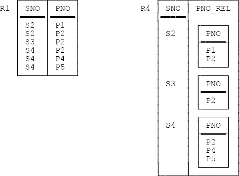
EXTEND S : { PQ ≔ !!SP }Suppose we evaluate this expression and assign the result to a relvar SPQ. A sample value for SPQ, corresponding to our usual sample values for relvars S and SP, is shown (in outline) in Figure 7-2 below. Attribute PQ is relation valued.
Now consider the following SQL expression:
SELECT SNO , SNAME , STATUS , CITY , PNO , QTY
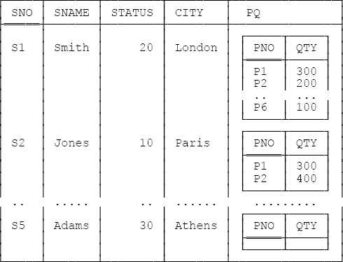
FROM S NATURAL LEFT OUTER JOIN SPThe result of evaluating this expression is shown (again in outline) in Figure 7-3 opposite.
Observe now that with our usual sample values, the set of shipments for supplier S5 is empty, and that:
In Figure 7-2, that empty set of shipments is represented by an empty set.
In Figure 7-3, by contrast, that empty set is represented by nulls (indicated by shading in the figure).
To represent an empty set by an empty set seems like such an obviously good idea! In fact, as I said earlier, there would be no need for outer join at all if RVAs were properly supported. Thus, one advantage of RVAs is that they deal more elegantly with the problem that outer join is intended to solve than outer join itself does—and I’m tempted to say that this fact all by itself, even if there were no other advantages, is a big argument in favor of RVAs.

At the risk of laboring the obvious, I’d like to say too that if there aren’t any shipments for supplier S5, it means, to repeat, that the set of shipments for supplier S5 is empty (and that’s exactly what the relation in Figure 7-2 says). It certainly doesn’t mean that supplier S5 supplies some unknown part in some unknown quantity; and yet unknown is—and in fact was originally and explicitly intended to be—the way null is usually interpreted. So Figure 7-3 not only involves nulls (which as we saw in Chapter 4 is bad news for all kinds of reasons), it actually misrepresents the semantics of the situation.
Let’s look at some typical operations involving relvar SPQ (Figure 7-2). Consider first the following queries:
As you can see, the natural language versions of these two queries are symmetric, but the Tutorial D formulations on the RVA design (Figure 7-2) aren’t. By contrast, Tutorial D formulations of the same queries against our usual (non RVA) design are symmetric, as well as being simpler than their RVA counterparts
( SP WHERE PNO = 'P2' ) { SNO }

( SP WHERE SNO = 'S2' ) { PNO }
In fact, the queries on the RVA design effectively involve mapping that design to the non RVA design anyway (that’s what the UNGROUPs do).
Similar remarks apply to updates and constraints. For example, suppose we need to update the database to show that supplier S2 supplies part P5 in a quantity of 500. Here are Tutorial D formulations on (a) the non RVA design, (b) the RVA design:
     INSERT SP RELATION { TUPLE { SNO 'S2' , PNO 'P5' , QTY 500 } } ;
     UPDATE SPQ WHERE SNO = 'S2' :
              { INSERT PQ RELATION { TUPLE { PNO 'P5' , QTY 500 } } } ;
Once again, the natural language requirement is stated in a symmetric fashion; its formulation in terms of the non RVA design is symmetric too; but its formulation in terms of the RVA design isn’t (in fact, it’s quite cumbersome). And, of course, the reason for this state of affairs is that the non RVA design itself is asymmetric—in effect, it regards parts as subordinate to suppliers, instead of giving parts and suppliers equal treatment, as it were.
Examples like the ones discussed above tend to suggest that RVAs in base relvars are probably a bad idea (certainly relvar SPQ in particular isn’t very well designed). But this position might better be seen as a guideline rather than an absolute limitation, because in fact there are cases—comparatively rare ones perhaps—where a base relvar with an RVA is exactly the right design. A sample value for such a relvar (SIBLING) is shown in Figure 7-4 below. The intended interpretation is that the persons identified within any given PERSONS value are all siblings of one another, and have no other siblings. Thus, Amy and Bob are siblings; Cal, Don, and Eve are siblings; and Fay is an only child. Note that the relvar has just one attribute (an RVA) and three tuples. Note too that the sole key involves an RVA.
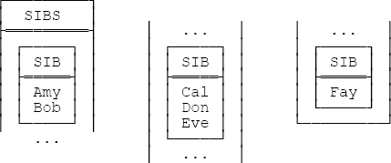
Note: It’s important to understand that no non RVA relation exists that represents exactly the same information, no more and no less, as the relation shown in Figure 7-4 does. In particular, if we ungroup that relation as follows—
SIBLING UNGROUP ( SIBS )
—we lose the information as to who’s the sibling of whom.
Consider once again this example from the section on image relations earlier in this chapter:
S WHERE ( !!SP ) { PNO } = P { PNO }(“suppliers who supply all parts”). Clearly, the boolean expression in the WHERE clause here involves a relational comparison (actually an equality comparison). Recall now from Chapter 6 that an expression of the form r WHERE bx denotes a restriction as such only if bx is a restriction condition, and bx is a restriction condition if and only if every attribute reference in bx identifies some attribute of r and there aren’t any relvar references. In the example, therefore, the boolean expression isn’t a genuine restriction condition, because (a) it involves some references to attributes that aren’t attributes of S and (b) it also involves some relvar references (to relvars SP and P). In fact, the example overall is really shorthand for something that might look like this:
     WITH ( R1 := EXTEND S  : { X := ( !!SP ) { PNO } } ,
            R2 := EXTEND R1 : { Y := P { PNO } } ) :
     R2 WHERE X = Y
Now the boolean expression in the WHERE clause (in the last line) is indeed a genuine restriction condition. Observe, however, that attributes X and Y are both RVAs. As the example suggests, therefore, RVAs are always involved, at least implicitly, whenever relational comparisons are performed.
Consider again relvar SPQ, with sample value as shown in Figure 7-2. Attribute PQ is relation valued. And just as it makes sense (and is useful) to define, e.g., numeric aggregate operators such as SUM on numeric attributes, so it makes sense, and is useful, to define relational aggregate operators on relation valued attributes. For example, the following expression returns the union of all of the relations currently appearing as values of attribute PQ in relvar SPQ
UNION ( SPQ , PQ )
Or equivalently (why exactly is this equivalent?):
UNION ( SPQ { PQ } )Tutorial D supports the following relation valued aggregate operators: UNION, D_UNION, and INTERSECT. And SQL has analogs of UNION and INTERSECT (though not D_UNION); however, they’re called, not UNION and INTERSECT as one might reasonably have expected, but FUSION and INTERSECTION [sic], respectively. (It would be very naughty of me to suggest that if union is called FUSION, then intersection ought surely to be called FISSION, so I won’t.)
[106] The double enclosing parentheses, both here and in the UNGROUP example, are necessary—the argument expression within the outer parentheses is a subquery, which requires parentheses of its own.