Here first are answers to certain exercises that were stated inline in the body of the chapter. In one, we were given relvars as follows—

     S   { SNO }        /* suppliers               */
     SP  { SNO , PNO }  /* supplier supplies part  */
     PJ  { PNO , JNO }  /* part is used in project */
     J   { JNO }        /* projects                */

—and we were asked for a SQL formulation of the query “Get all (sno,jno) pairs such that sno appears in S, jno appears in J, and supplier sno supplies all parts used in project jno.” A possible formulation is as follows:

     SELECT SX.SNO , JX.JNO
     FROM   S AS SX , J AS JX
     WHERE  NOT EXISTS
          ( SELECT *
            FROM   P AS PX
            WHERE  EXISTS
                 ( SELECT *
                   FROM   PJ AS PJX
                   WHERE  PJX.PNO = PX.PNO
                   AND    PJX.JNO = JX.JNO )
            AND    NOT EXISTS
                 ( SELECT *
                   FROM   SP AS SPX
                   WHERE  SPX.PNO = PX.PNO
                   AND    SPX.SNO = SX.SNO ) )

Note: For a detailed discussion of how to tackle complicated queries like this one in SQL, see Chapter 11.

Another inline exercise asked what happens if (a) r1 and r2 are relations with no attribute names in common, (b) r2 is empty, (c) we form the product r1 TIMES r2, and finally (d) we divide that product by r2. Answer: It should be clear that the product is empty, and hence the final result is empty too (it has the same heading as r1, but of course it isn’t equal to r1, in general). Do note, however, that dividing by an empty relation isn’t an error (it’s not like dividing by zero in arithmetic).

Another inline exercise asked why the following Tutorial D and SQL expressions weren’t quite equivalent:

     S WHERE SUM ( !!SP , QTY ) < 1000
     SELECT S.*
     FROM   S , SP
     WHERE  S.SNO = SP.SNO
     GROUP  BY S.SNO , S.SNAME , S.STATUS , S.CITY
     HAVING SUM ( SP.QTY ) < 1000

The difference is that the Tutorial D expression will return a result that includes suppliers (like supplier S5, given our usual sample data values) who supply no parts at all, but the SQL expression won’t. Subsidiary exercise: What accounts for the discrepancy?

7.1 Throughout these answers, I show SQL expressions that aren’t necessarily direct transliterations of their algebraic counterparts but are, rather, “more natural” formulations of the query in SQL terms. The solutions aren’t necessarily unique. Note: This latter remark applies to many of the code solutions throughout the remainder of this appendix, and I won’t bother to make it again.

7.2 The expressions r1 MATCHING r2 and r2 MATCHING r1 are equivalent if and only if r1 and r2 are of the same type, in which case both expressions reduce to just JOIN{r1,r2} (and this latter expression reduces in turn to INTERSECT{r1,r2}).

7.3 RENAME isn’t primitive because (for example) the expressions

     S RENAME { CITY AS SCITY }

and

     ( EXTEND S : { SCITY := CITY } ) { ALL BUT CITY }

are equivalent. Note: Possible appearances to the contrary notwithstanding, EXTEND isn’t primitive either—it can be defined in terms of join (at least in principle), as is shown in the book Databases, Types, and the Relational Model: The Third Manifesto, by Hugh Darwen and myself (see Appendix G).

7.4 EXTEND S { SNO } : { NP := COUNT ( !!SP ) }

7.5 You can determine which of the expressions are equivalent to which by inspecting the following results of evaluating them. Note that the “summary” SUM(1), evaluated over n tuples, is equal to n. (Even if n is zero! SQL, of course, would say the result is null in such a case.)

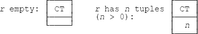
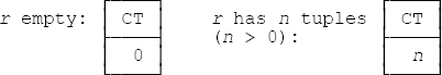
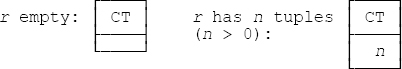
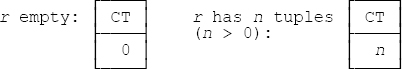
In other words, the result is a relation of degree one in every case. If r is nonempty, all four expressions are equivalent; otherwise a. and c. are equivalent, and b. and d. are equivalent. SQL analogs:

7.6 They return, respectively, the empty relation and the universal relation (of the applicable type in each case). Note: The universal relation of type RELATION{H} is the relation of that type that contains all possible tuples of type TUPLE{H}. The implementation might reasonably want to outlaw invocations of INTERSECT on an empty argument (at least if those invocations really need the result to be materialized).

Just to remind you, SQL’s analogs of the UNION and INTERSECT aggregate operators are called FUSION and INTERSECTION, respectively. If their arguments are empty, they both return null. Otherwise, they return a result as follows (these are direct quotes from the standard; T is the table over which the aggregation is being done). First FUSION:

(The “element type” is the type of the elements of the multisets in the argument column.) Now INTERSECTION:

Note the asymmetry, incidentally: In SQL, INTERSECTION (and INTERSECT) are defined in terms of MIN, but FUSION (and UNION) are defined in terms not of MAX but of SUM (?).

7.7 The predicate can be stated in many different ways, of course. Here’s one reasonably straightforward formulation: Supplier SNO supplies part PNO if and only if part PNO is mentioned in relation PNO_REL. That “and only if” is important, by the way (right?).

7.8 Relation r has the same cardinality as SP and the same heading, except that it has one additional attribute, X, which is relation valued. The relations that are values of X have degree zero; furthermore, each is TABLE_DEE, not TABLE_DUM, because every tuple sp in SP effectively includes the 0-tuple as its value for that subtuple of sp that corresponds to the empty set of attributes. Thus, each tuple in r effectively consists of the corresponding tuple from SP extended with the X value TABLE_DEE, and the original GROUP expression is logically equivalent to the following:

     EXTEND SP : { X := TABLE_DEE }

The expression r UNGROUP (X) yields the original SP relation again.

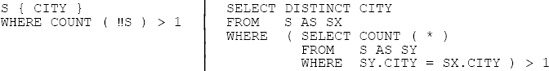
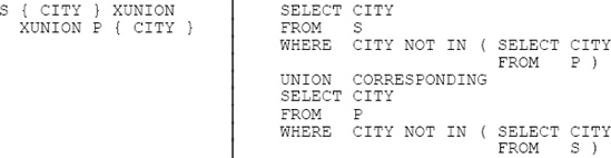
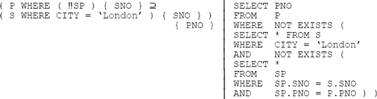
7.9 Tutorial D on the left, SQL on the right as usual:

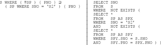
7.10 It’s the same as TCLOSE (pp). In other words, transitive closure is idempotent. Note: I’m extending the definition of idempotence slightly here. In Chapter 6, I said (in effect) that a dyadic operator Op is idempotent if and only if x Op x = x for all x; now I’m saying (in effect) that a monadic operator Op is idempotent if and only if Op(Op(x)) = Op(x) for all x.

7.11 It denotes a relation looking like this (in outline):

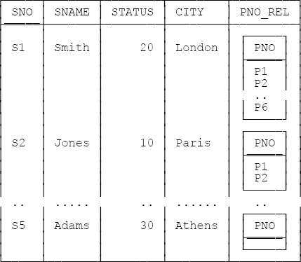
The expression is logically equivalent to the following:

     ( S JOIN SP { SNO , PNO } ) GROUP ( { PNO } AS PNO_REL )

Attribute PNO_REL is an RVA. Note, incidentally, that if r is the foregoing relation, then the expression

     ( r UNGROUP ( PNO_REL ) ) { ALL BUT PNO }

will not return our usual suppliers relation. To be precise, it will return a relation that differs from our usual suppliers relation only in that it’ll have no tuple for supplier S5.

7.12 The first is straightforward: It inserts a new tuple, with supplier number S6, name Lopez, status 30, city Madrid, and PNO_REL value a relation containing just one tuple, containing in turn the PNO value P5. As for the second, I think it would be helpful to repeat from Appendix D the Tutorial D grammar for <relation assign> (the names of the syntactic categories are meant to be self-explanatory):

     <relation assign>
         ::=   <relvar name> := <relation exp>
             | <insert> | <d_insert> | <delete> | <i_delete> | <update>
     <insert>
         ::=   INSERT <relvar name> <relation exp>

     <d_insert>
         ::=   D_INSERT <relvar name> <relation exp>

     <delete>
         ::=   DELETE <relvar name> <relation exp>
             | DELETE <relvar name> [ WHERE <boolean exp> ]

     <i_delete>
         ::=   I_DELETE <relvar name> <relation exp>

     <update>
         ::=   UPDATE <relvar name> [ WHERE <boolean exp> ] :
                                    { <attribute assign commalist> }

And an <attribute assign>, if the attribute in question is relation valued, is basically just a <relation assign> (except that the pertinent <attribute name> appears in place of the target <relvar name> in that <relation assign>), and that’s where we came in. Thus, in the exercise, what the second update does is replace the tuple for supplier S2 by another in which the PNO_REL value additionally includes a tuple for part P5.

7.13 Query a. is easy:

     WITH ( X := ( SSP RENAME { SNO AS XNO } ) { XNO , PNO_REL } ,
            Y := ( SSP RENAME { SNO AS YNO } ) { YNO , PNO_REL } ) :
     ( X JOIN Y ) { XNO , YNO }

Note that the join here is being done on an RVA (and so is implicitly performing relational comparisons).

Query b., by contrast, is not so straightforward. Query a. was easy because SSP “nests parts within suppliers,” as it were; for Query b. we would really like to have suppliers nested within parts instead. So let’s do that:^[205]

     WITH ( PPS := ( SSP UNGROUP ( PNO_REL ) ) GROUP ( { SNO } AS SNO_REL ) ,
            X   := ( PPS RENAME { PNO AS XNO } ) { XNO , SNO_REL } ,
            Y   := ( PPS RENAME { PNO AS YNO } ) { YNO , SNO_REL } ) :
     ( X JOIN Y ) { XNO , YNO }
7.14 WITH ( R1 := P RENAME { WEIGHT AS WT } ,
      R2 := EXTEND P : { N_HEAVIER :=
                         COUNT ( R1 WHERE WT > WEIGHT ) } ) :
     ( R2 WHERE N_HEAVIER < 2 ) { ALL BUT N_HEAVIER }

SELECT *
FROM   P AS PX
WHERE ( SELECT COUNT ( * )
        FROM   P AS PY
        WHERE  PX.WEIGHT < PY.WEIGHT ) < 2

Both formulations return parts P2, P3, and P6 (i.e., a result of cardinality three, even though the specified quota was two). Quota queries can also return a result of cardinality less than the specified quota (e.g., consider the query “Get the ten heaviest parts”).

Note: Quota queries are quite common in practice. In our book Databases, Types, and the Relational Model: The Third Manifesto (see Appendix G), therefore, Hugh Darwen and I suggest a shorthand for expressing them, according to which the foregoing query might be expressed thus in Tutorial D:

     ( ( RANK P BY ( DESC WEIGHT AS W ) ) WHERE W ≤ 2 ) { ALL BUT W }

SQL has something similar.

7.15 This formulation does the trick:

     SUMMARIZE SP { SNO , QTY } PER ( S { SNO } ) : { SDQ := SUM ( QTY ) }

But the following formulation, using EXTEND and image relations, is surely to be preferred:

     EXTEND S { SNO } : { SDQ := SUM ( !!SP { QTY } }

Here for interest is an SQL analog:

     SELECT SNO ,
          ( SELECT COALESCE ( SUM ( DISTINCT QTY ) , 0 ) AS SDQ
     FROM   S
7.16  EXTEND S : { NP := COUNT ( !!SP ) , NJ := COUNT ( !!SJ ) }

JOIN { S , SUMMARIZE SP PER ( S { SNO } ) : { NP := COUNT ( PNO ) } ,
           SUMMARIZE SJ PER ( S { SNO } ) : { NJ := COUNT ( JNO ) } }

SELECT SNO , ( SELECT COUNT ( PNO )
               FROM   SP
               WHERE  SP.SNO = S.SNO ) AS NP ,
             ( SELECT COUNT ( JNO )
               FROM   SJ
               WHERE  SJ.SNO = S.SNO ) AS NJ
FROM   S

7.17 For a given supplier number, sno say, the expression !!SP denotes a relation with heading {PNO,QTY} and body consisting of those (pno,qty) pairs that correspond in SP to that supplier number sno. Call that relation ir (for image relation). By definition, then, for that supplier number sno, the expression !!(!!SP) is shorthand for the following:

     ( ( ir ) MATCHING RELATION { TUPLE { } } ) { ALL BUT }

This expression in turn is equivalent to:

     ( ( ir ) MATCHING TABLE_DEE ) { PNO , QTY }

And this expression reduces to just ir. Thus, “!!“ is idempotent (i.e., !!(!!r) is equivalent to !!r for all r), and the overall expression

     S WHERE ( !!(!!SP) ) { PNO } = P { PNO }

is equivalent to:

     S WHERE ( !!SP ) { PNO } = P { PNO }

(“Get suppliers who supply all parts”).

7.18 No, there’s no logical difference.

7.19 S JOIN SP isn’t a semijoin; S MATCHING SP isn’t a join (it’s a projection of a join). The expressions r1 JOIN r2 and r1 MATCHING r2 are equivalent if and only if relations r1 and r2 are of the same type (when the final projection becomes an identity projection, and the expression overall degenerates to r1 INTERSECT r2).

7.20 If r1 and r2 are of the same type and t1 is a tuple in r1, the expression !!r2 (for t1) denotes a relation of degree zero—TABLE_DEE if t1 appears in r2, TABLE_DUM otherwise. And if r1 and r2 are the same relation (r, say), !!r2 becomes !!r, and it denotes TABLE_DEE for every tuple in r.

7.21 They’re the same unless table S is empty, in which case the first yields a one-column, one-row table containing a zero and the second yields a one-column, one-row table “containing a null.”

7.22 In SQL, typically in a cursor definition; in Tutorial D (where ORDER BY is spelled just ORDER), in a special operator (“LOAD”), not discussed further in this book, that retrieves a specified relation into an array (of tuples).