Before I get to the join operator as such, it’s helpful to introduce the concept of “joinability.” Relations r1 and r2 are joinable if and only if attributes with the same name are of the same type (meaning they are in fact the very same attribute)—equivalently, if and only if the set theory union of the headings of r1 and r2 is itself a legal heading. Note that this concept applies not just to join as such but to various other operations as well, as we’ll see in the next chapter. Anyway, armed with this notion, I can now define the join operation (note how the definition appeals to the fact that tuples are sets and hence can be operated upon by set theory operators such as union):
Definition: Let relations r1 and r2 be joinable. Then their natural join (or just join for short), r1 JOIN r2, is a relation with (a) heading the set theory union of the headings of r1 and r2 and (b) body the set of all tuples t such that t is the set theory union of a tuple from r1 and a tuple from r2.
The following example is repeated from the section SOME PRELIMINARIES, except that now I’ve dropped the explicit name qualifiers in the SQL version where they aren’t needed:
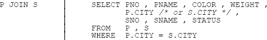
I remind you, however, that SQL also allows this join to be expressed in an alternative style that’s a little closer to that of Tutorial D (and this time I deliberately replace that long commalist of column references in the SELECT clause by a simple “*”):
     SELECT *
     FROM   P NATURAL JOIN S
The result heading, given this latter formulation, has attributes—or columns, rather—CITY, PNO, PNAME, COLOR, WEIGHT, SNO, SNAME, and STATUS (in that order in SQL, though not of course in the Tutorial D analog).
There are several more points to be made in connection with the natural join operation. First of all, observe that intersection is a special case (i.e., r1 INTERSECT r2 is a special case of r1 JOIN r2, in Tutorial D terms). To be specific, it’s the special case in which relations r1 and r2 aren’t merely joinable but are actually of the same type (i.e., have the same heading). For example, the following expressions are logically equivalent
     P { CITY } INTERSECT S { CITY }
     P { CITY } JOIN S { CITY }
However, I’ll have more to say about INTERSECT as such later in this chapter.
Next, product is a special case, too (i.e., r1 TIMES r2 is a special case of r1 JOIN r2, in Tutorial D terms). To be specific, it’s the special case in which relations r1 and r2 have no attribute names in common. Why? Because, in this case, (a) the set of common attributes is empty; (b) as noted earlier, every possible tuple has the same value for the empty set of attributes (namely, the 0-tuple); thus, (c) every tuple in r1 joins to every tuple in r2, and so we get the product as stated. For example, the following expressions are logically equivalent:
     P { ALL BUT CITY } TIMES S { ALL BUT CITY }
     P { ALL BUT CITY } JOIN S { ALL BUT CITY }
For completeness, however, I’ll give the definition anyway:
Definition: The cartesian product (or just product for short) of relations r1 and r2, r1 TIMES r2, where r1 and r2 have no common attribute names, is a relation with (a) heading the set theory union of the headings of r1 and r2 and (b) body the set of all tuples t such that t is the set theory union of a tuple from r1 and a tuple from r2.
Here’s an example:
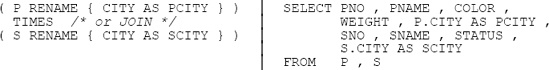
Note the need to rename at least one of the two CITY attributes in this example. The result heading has attributes or columns PNO, PNAME, COLOR, WEIGHT, PCITY, SNO, SNAME, STATUS, and SCITY (in that order, in SQL).
Last, join is usually thought of as a dyadic operator specifically; however, it’s possible, and useful, to define an n-adic version of the operator (and Tutorial D does), according to which we can write expressions of the form
JOIN { r1 , r2 , ... , rn }to join any number of relations r1, r2, ..., rn.[78] For example, the join of parts and suppliers could alternatively be expressed as follows:
JOIN { P , S }What’s more, we can use this syntax to ask for “joins” of just a single relation, or even of no relations at all! The join of a single relation r, JOIN {r}, is just r itself; this case is perhaps not of much practical importance (?). Perhaps surprisingly, however, the join of no relations at all, JOIN {}, is very important indeed!—and the result is TABLE_DEE. (Recall once again that TABLE_DEE is the unique relation with no attributes and just one tuple.) Why is the result TABLE_DEE? Well, consider the following:
In ordinary arithmetic, 0 is what’s called the identity (or identity value) with respect to “+”; that is, for all numbers x, the expressions x + 0 and 0 + x are both identically equal to x. As a consequence, the sum of no numbers is 0.[79] (To see this claim is reasonable, consider a piece of code that computes the sum of n numbers by initializing the sum to 0 and then iterating over those n numbers. What happens if n = 0?)
In like manner, 1 is the identity with respect to “*”; that is, for all numbers x, the expressions x * 1 and 1 * x are both identically equal to x. As a consequence, the product of no numbers is 1.
In the relational algebra, TABLE_DEE is the identity with respect to JOIN; that is, for all relations r, the expressions r JOIN TABLE_DEE and TABLE_DEE JOIN r are both identically equal to r (see the paragraph immediately following). As a consequence, the join of no relations is TABLE_DEE.
If you’re having difficulty with this idea, don’t worry about it too much for now. But if you come back to reread this section later, I do suggest you try to convince yourself that r JOIN TABLE_DEE and TABLE_DEE JOIN r are indeed both identically equal to r. It might help to point out that the joins in question are actually cartesian products (right?).
In SQL, the keyword JOIN can be used to express various kinds of join operations (although those operations can always be expressed without it, too). Simplifying slightly, the possibilities—I’ve numbered them for purposes of subsequent reference—are as follows (t1 and t2 are tables, denoted by table expressions tx1 and tx2, say; bx is a boolean expression; and C1, C2, ..., Cn are columns appearing in both t1 and t2):
t1NATURAL JOINt2t1JOINt2ONbxt1JOINt2USING (C1,C2, ... ,Cn)t1CROSS JOINt2
I’ll elaborate on the four cases briefly, since the differences between them are a little subtle and can be hard to remember:
Case 1 has effectively already been explained. Note: Actually, Case 1 is logically identical to a Case 3 expression—see below—in which the specified columns C1, C2, ..., Cn are all of the common columns (i.e., all of the columns that appear in both t1 and t2), in the order in which they appear in t1.
Case 2 is logically equivalent to the following:
( SELECT * FROM
t1,t2WHEREbx)Case 3 is logically equivalent to a Case 2 expression in which bx takes the form
t1.C1=t2.C1ANDt1.C2=t2.C2AND ... ANDt1.Cn=t2.Cn—except that columns C1, C2, ..., Cn appear once, not twice, in the result, and the column ordering in the heading of the result is (in general) different: Columns C1, C2, ..., Cn appear first, in that order; then the other columns of t1 appear, in the order in which they appear in t1; then the other columns of t2 appear, in the order in which they appear in t2. (Do you begin to see what a pain this left to right ordering business is?)
Finally, Case 4 is logically equivalent to the following:
( SELECT * FROM
t1,t2)
Recommendations:
Use Case 1 (NATURAL JOIN) in preference to other methods of formulating a join (but make sure columns with the same name are of the same type). Note that the NATURAL JOIN formulation will often be the most succinct if other recommendations in this book are followed.[80]
Avoid Case 2 (JOIN ON), because it’s guaranteed to produce a result with duplicate column names (unless tables t1 and t2 have no common column names in the first place). But if you really do want to use Case 2—which you just might, if you want to formulate a greater-than join, say[81]—then make sure columns with the same name are of the same type, and make sure you do some appropriate renaming as well. For example:
     SELECT TEMP.*
     FROM ( SELECT * FROM S JOIN P ON S.CITY > P.CITY ) AS TEMP
          ( SNO , SNAME , STATUS , SCITY ,
            PNO , PNAME , COLOR , WEIGHT , PCITY )
It’s not really clear why you’d ever want to use such a formulation, however, given that it’s logically equivalent to the following slightly less cumbersome one:
     SELECT SNO , SNAME , STATUS , S.CITY AS SCITY ,
            PNO , PNAME , COLOR , WEIGHT , P.CITY AS PCITY
     FROM   S , P
     WHERE  S.CITY > P.CITY
In Case 3, make sure columns with the same name are of the same type.
In Case 4, make sure there aren’t any common column names.
Recall finally that as noted in Chapter 1 an explicit JOIN invocation isn’t allowed in SQL as a “stand alone” table expression (i.e., one at the outermost level of nesting). Nor is it allowed as the table expression in parentheses that constitutes a subquery (see Chapter 12).
[78] For usability reasons, Tutorial D also supports n-adic versions of INTERSECT and TIMES. I’ll skip the details here.
[79] As noted in Chapter 4, the SQL “set function” SUM yields null, not zero, if it’s invoked on a set of no numbers. But this is just a logical mistake on the part of SQL—it has no bearing on the present discussion.
[80] Perhaps I should inject a small note of caution here. In practice, it’s very common for SQL tables to have some kind of “comments” column; thus, there’s a risk that NATURAL JOIN might produce unexpected results, unless some appropriate naming discipline is followed (or some appropriate renaming is done) in connection with such columns.
[81] Greater-than join is a special case of what’s called θ-join, which I’ll be discussing later in this chapter.