Chapter 6. Keeping your source code files elegant

This chapter covers

• Distributing complexity
• Lack of Cohesion of Methods: files that do too much
• RFC and couplings: classes with too many friends

An active project gets bigger day by day, week by week. As your software grows, it becomes more complex. New classes are added, and methods and attributes are created or improved. Each time you make a change, you’re probably affecting the health of your system’s design. Whenever logic is added, the complexity of the file, the package, and the module is increased.

Fortunately, SonarQube can alert you to these kinds of issues. For instance, it can tell you when the quality of your design goes down, when the increasing complexity of a file starts to make it hard to maintain, or when the time comes to break up this complexity without reducing the overall complexity.

In this chapter, we’ll look at complexity—not from a system-level perspective, but at the level of individual files. How internally complex is the average file in your system? How complex are its interactions with the rest of your system? Both questions are important because they help you gauge how difficult the average file is to work on and how broad an impact (good or bad) working on that file will have on the rest of your system. Unless you’re familiar with a given system, you probably don’t know offhand where its “worst” classes are, but SonarQube can help you find those trouble spots and prioritize them for refactoring.

We’ll begin by looking at class-level complexity (known as cyclomatic complexity, or the McCabe metric). Then we’ll move back a step to look at Lack of Cohesion of Methods (LCOM), which takes a more abstract view of each class to ask, “Is this class doing too much?”

After that, we’ll move on to the complexity of interactions with Response for Class (RFC), which looks at how a file interacts in a system, and at afferent and efferent couplings, which also fall under the “complexity of interactions” heading. We’ll show you how to identify poorly designed classes, discuss refactoring methods, and give you some tips on keeping your source code clean and simple.

6.1. Keeping complexity low

Sam, the junior developer on the team, is still smarting from giving an over-optimistic estimate on her last assignment. She’s eager to redeem herself when she’s told to change the validation algorithm for Visa credit cards. Visa recently changed the rules for what’s valid, and the deadline to have the new validation in place is looming.

Unfortunately, validation for every credit card type the system accepts (American Express, Discover, Diners, MasterCard, Visa, and so on) is handled through the same huge class. Worse, most of it runs through one monster method packed with more spaghetti than an Italian restaurant. Sam knows it should be structured differently, but she doesn’t have the time or (she’s afraid) the experience to restructure the code. Instead, she spends several hours—with her restless boss asking constantly about her progress—just reading the code.

She finishes near the end of the day, just ahead of the deadline, but nobody is happy. What should have taken less than two hours took a whole day, and even her boss has to admit that it’s not Sam’s fault. The class was too complex, and she needed lots of time to read the code and become familiar with it before modifying it.

This section teaches you how to spot complex files by using SonarQube. It explains why it’s important to keep the complexity as low as you can, and describes briefly how complexity is calculated. At the end, we give you some refactoring tips, and we show how you can minimize the complexity value without changing the output of your code.

6.1.1. Hunting those huge files

Modifying highly complex files like Sam had to do is an error-prone process. Some studies have shown that as complexity rises, so does bugginess. Sam went slowly, and rightly so, because a high level of complexity decreases a file’s maintainability and increases the time it takes to understand the code. The harder it is to completely take in a method or file, the more likely you are to subtly (or not so subtly) screw it up when you work on it. Additionally, high complexity makes it difficult to properly unit-test a method; that’s why most of the time, using a Test-Driven Development approach prevents developers from generating such complex methods.

How is complexity defined? Is it like the Supreme Court’s take on pornography—you know it when you see it? Maybe, but believe it or not, it’s also measurable. It’s more complicated than this, but loosely, you can think of complexity as the count of pairs of curly braces (real or implied) in a class or method. That’s the McCabe metric, commonly called cyclomatic complexity, which SonarQube reports in the complexity widget shown in figure 6.1.

Figure 6.1. Dashboard complexity widget

The numbers in the widget are averages: average complexity per method, class, and file. The number at the bottom is the application’s overall complexity, which is a sum of the parts. The graph on the right side of the widget shows the distribution of complexity across either methods or files, based on which radio button is selected.

Because you want to see that graph weighted to the left, the project reflected in figure 6.1 looks pretty good. But switch it to show the complexity distribution across files, as shown in figure 6.2, and the picture changes—literally.

Figure 6.2. Files distribution/complexity bar chart

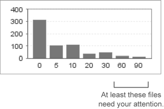
Suddenly that smooth, pretty slope has a spike on the right side. What’s this telling us? The first graph shows that most methods have low complexity, and the second one indicates that some files (five, to be exact) have high complexity. This likely means a handful of files have lots and lots of methods. Because getters and setters aren’t counted in the complexity equations, you know the spike in the graph doesn’t merely reflect classes with a lot of members. No, these are files with a lot going on.

Because high complexity makes a file harder to maintain, you should consider refactoring any file with a complexity of 60 or more, whether that complexity comes from 2 methods with complexity scores of 30 each, or 10 methods each with a score of 6. In the first case, both methods are complicated; but in the second case, the class probably has too many methods. Tracking methods with too-high complexity is important, and in that case, you should activate some rules to get issues and track those methods that are candidates for refactoring (see Chapter 12 for more details).

Either way, these five files definitely need to be examined, but you’ll have to look inside the file to decide your next steps. That’s where the drilldown comes in. Click-through on the metric of your choice (probably complexity per file) to get there. Once you’ve landed at the drilldown, the normal worst-first sorting brings the worst offenders to the top. Choose a file, and you’ll find yourself on the Source tab. There is no special tab in the file detail view for complexity, but the file’s complexity metrics appear in the Source tab header, as shown in figure 6.3.

Figure 6.3. Complexity metrics shown in source code viewer default tab

Okay, so now what? You know the class is a problem, but what do you do with it? To answer that, we’ll look at what these numbers actually mean—how they’re computed—and then we’ll talk about refactoring strategies.

6.1.2. Complexity: what it looks like and how to fix it

We said earlier that cyclomatic complexity can be thought of as the count of pairs of curly braces. But it’s more complicated than that. Early returns figure in, as do multiple conditions (&&s and ||s) in control structures (ifs and whiles.) It’s best explained with an example, like the following listing.

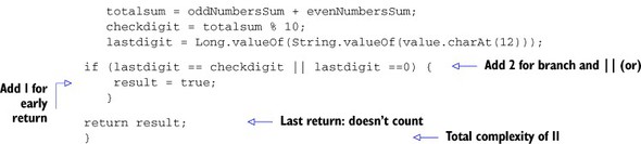
Listing 6.1. Example of code that is too complex

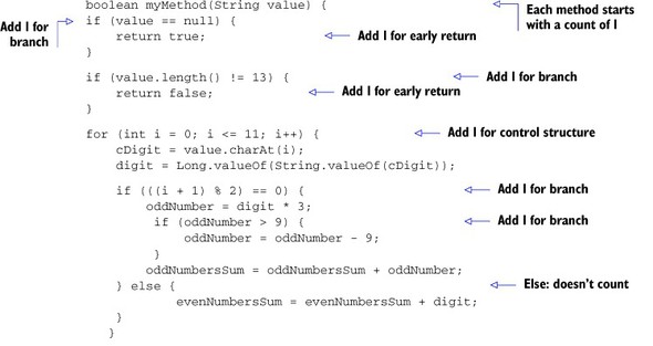
Cyclomatic complexity can be calculated for any fraction of source code (method, function, class, file, module, and so on). It counts the number of possible paths (branches) through the source code.

By default, every method has a complexity value of 1. For Java, the following keywords and statements are considered branches and add one point to the complexity: case, catch, for, if, throw, while, &&, ||, the ternary operator ? (which is just a fancy if), and return, except for the last one in a method. If you manually compute the complexity of the code in listing 6.1, you’ll get a value of 11 points, which comes from the default value (+1), 5 ifs (+5), 3 early returns (+3), 1 for loop (+1), and 1 || (+1).

Listing 6.2 shows another example: a method that gets an array of integers and returns a count of array items that are divisible by four. If the array is empty, then an IllegalArgumentException is thrown.

Listing 6.2. Method that checks how many numbers are divisible by 4

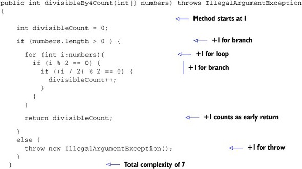
The cyclomatic complexity of the divisibleBy4Count() method comes to 7. Note that even though there’s only one return, it increases the complexity of the method because it doesn’t come at the end of the method. The compiler might smooth out that little wrinkle, but it still makes the method harder to take in, and that’s what you’re trying to calculate.

The SonarSource folks suggest refactoring a method when its complexity is greater than 7. The method in listing 6.2 weighs in at 7, just under the threshold, but it’s obvious that the method can be improved. You can remove the assertion of an empty array by introducing a new method for performing this check. The new version of the code looks like this.

Listing 6.3. Revised method that checks how many numbers are divisible by 4

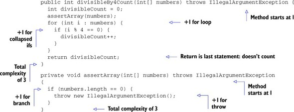
Manually calculating the complexity for each method, you get the following results:

• divisibleBy4Count() = 3
• assertArray() = 3

The refactoring accomplished a couple of things. First, we reduced complexity by refactoring the basic algorithm. This was a trivial example, but we hope it makes the point that basic improvements like this are often possible. Second, we demonstrated reducing complexity and improving readability by distributing the complexity of one method across multiple methods.

Now that we’ve looked at cyclomatic complexity, we’ll move on to a slightly more abstract metric, which looks at the complexity of what the class is trying to do.

6.2. Lack of Cohesion of Methods: files that do too much

Earlier, we talked about two theoretical classes with a cyclomatic complexity of 60 each: one with 10 methods that each scored 6, and one with 2 methods scoring 30 each. We’ve already looked at how to approach the class with two large methods.

The next metric we’ll look at, Lack of Cohesion of Methods (LCOM), helps address the class with lots of methods. At the time of this writing, the metric is only available for Java projects, but sooner or later more languages’ plugins will compute this metric. First we’ll discuss the widget that reports on the metric and why it’s not shown in the default dashboard. Then we’ll show you the source code tab viewer that presents the LCOM of a class in a nice, clean way. After that, it’s time for coding. Through a short example, you’ll compute the LCOM metric of a simple class; then you’ll try to refactor it to improve it.

6.2.1. Getting reports about the LCOM metric

At its root, LCOM is the count of the number of responsibilities a class has. There are several variations on the LCOM algorithm. SonarQube uses LCOM4, the fourth one to be published, because it’s the most convenient for computations in real source code. The previous versions are used in scientific and research circles, but not in the field.

Although complexity is one of SonarQube’s Seven Axes of Quality, the related widgets aren’t included in SonarQube’s default dashboard because the metrics are considered “too hard.” The thinking is that for the majority of SonarQube users, the widgets would only add noise to the dashboard. This won’t apply to you, because after reading this chapter you’ll have a thorough understanding of how these metrics are computed and what they tell you about your source code.

Before we get to the meat, you should add the LCOM4 widget to your dashboard. Chapter 14 gives you low-level details on how, but if you’re logged in as an administrator, you’ll find an intuitive interface behind the Configure Widgets link at upper right on any dashboard. While you’re at it, add the Response for Class widget, too. You don’t need it for this section, but you’ll want it for the next one. The two target widgets are filed in the Design widget category, and you can see a preview of them in figure 6.4. Don’t be surprised that they already have data. Even though the widgets weren’t included on your dashboard, SonarQube has been calculating these values all along, so the normal “changes take effect after the next analysis” rule doesn’t apply here.

Figure 6.4. LCOM4 and RFC metrics shown in dashboard widgets

The primary number in each of these widgets is the metric’s average per class across the project, and the graphs represent a complexity distribution. In general, you want the numbers to be low and the graphs weighted to the left. For LCOM4, you also see the density of suspect files—those with LCOM more than 1. As you’ll see, every file with LCOM >= 2 is a candidate for refactoring.

From the dashboard, click any of the LCOM4 numbers (or the LCOM4 graph) to get to the drilldown view. You’ll get the standard drilldown behavior: only files or classes that need work, sorted worst first. Click a class, and SonarQube reports on the LCOM4 value for individual files in an LCOM4 tab with a graphic presentation of connected components, as shown in figure 6.5.

Figure 6.5. SonarQube reports on LCOM4 with a separate tab in the file source code viewer. The beauty of the LCOM4 tab is that you get a visual representation of which methods (an m in a reddish circle) are connected to which fields (an f in a yellow circle), and how the relations are formed.

“But what does this mean?” you may be wondering. Let’s find out.

6.2.2. Counting responsibilities

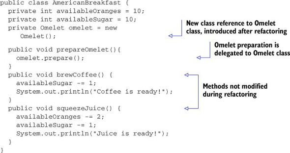
We could try to explain LCOM4, but the best way to give you a fundamental understanding of it is to show how you’d compute it by hand in a simple class. Listing 6.4 shows a simple AmericanBreakfast class with some local members and several methods accessing them. The purpose of the class is to prepare an American breakfast, update the availability of the materials, and print a message. A client would probably use some or all of the public methods provided to prepare a partial or complete breakfast. This code is a good example of a class with LCOM4 > 1, because its first version has more than one responsibility.

Listing 6.4. AmericanBreakfast class with LCOM4 > 1

public class AmericanBreakfast {
  private int availableOranges = 10;
  private int availableEggs = 5;
  private int availableBacon = 4;
  private int availableSugar = 10;
  private int availableSalt = 10;

  public void prepareOmelet(){
    fryBacon();
    bakeEggs();
    availableSalt-=1;
    System.out.println ("Omelet is ready!");

  }
  public void brewCoffee(){
    availableSugar -=1;
    System.out.println ("Coffee is ready!");
  }
  private void bakeEggs(){
    availableEggs -=2;
  }
  private void fryBacon(){
     availableBacon -=1;
  }
  public void squeezeJuice(){
    availableOranges -=2;
    availableSugar -=1;
    System.out.println ("Juice is ready!");
  }
}

LCOM4 counts the class’s responsibilities by looking at its methods and members and grouping together ones that are connected. (Kind of like the six degrees of Kevin Bacon, except that you don’t care how many degrees there are.)

All class members used in a given method are seen as being connected to both the method itself and to each other. If another method uses those same fields (or some subset of them), then it’s connected to those members and to the first method as well; it’s added to the relation connection. If it uses totally different members, it forms a new, unrelated connection with those other members. Methods can be also considered connected if one calls another and vice versa.

To sum up, two methods (m1 and m2) are grouped together if at least one of the following is true:

• Method m1 invokes method m2, or method m2 invokes method m1.
• Both methods (m1 and m2) use at least one of the same class attributes.

The AmericanBreakfast class in listing 6.4 has five members and several methods. Let’s look at how many concrete (unrelated) components exist in the class; in other words, let’s calculate the LCOM4.

The prepareOmelet() method invokes bakeEggs() and fryBacon() and uses the attribute availableSalt, so all three methods and the availableSalt member belong to the same group. Further, bakeEggs() and fryBacon() access the availableEggs and availableBacon members. Based on the previous definition, you need to add the two methods and both members to the group just identified.

Now look at the remaining public methods: brewCoffee() and squeezeJuice(). They’re connected because they use the availableSugar attribute. Notice that you also need to add the availableOranges property to this group because it’s accessed by the squeezeJuice() method. You might argue that you don’t add sugar to your orange juice; well, we don’t either, but it’s a good way to get the kids to drink up without complaint. Also, it works great in this example! It’s obvious that these two methods have no relation with the first group, so they form a new component.

Figure 6.6 shows graphically what we’ve just walked through—which, by the way, yields an LCOM4 of 2 for the AmericanBreakfast class we’re examining.

Figure 6.6. Connected methods and attributes of the AmericanBreakfast class

So, what’s the best LCOM4 score? It’s 1. This means all the methods and members in a class are well connected to each other and the class adheres to the Single Responsibility Principle, which as you might guess says that a class should have only one responsibility. A value of 0 implies a class with no methods, not even setters and getters, such as package-info.java. In other words, it’s a file with no code in it. And any value higher than 1 indicates that the class is a candidate for refactoring. Notice that we used the word candidate. In a minute, we’ll show you why an LCOM4 value greater than 1 doesn’t always mean bad design.

6.2.3. Refactoring for fewer responsibilities

With an LCOM4 score of 2, the AmericanBreakfast class is a candidate for refactoring. This means it breaks the Single Responsibility Principle because it’s responsible for two tasks: preparing an omelet and fixing drinks. Let’s refactor the class to minimize its LCOM4 score. There are two ways to go about this: split the class by responsibility, or add cohesion (which could be a hack, depending on the circumstances). If an American breakfast always contains orange juice, coffee, and an omelet, then you want to go the “add cohesion” route and prevent the client from calling classes that prepare only a portion of the breakfast. To do that, you make all the methods private, and add a new public method like so:

public void prepare(){
  prepareOmelet();
  brewCoffee();
  squeezeJuice();

Running a new SonarQube analysis gives an LCOM4 score of 1 for the class because the new prepare() method has tied together the formerly unconnected component groups, as figure 6.7 illustrates.

Figure 6.7. By tying together the separate components, you make the class comply with the Single Responsibility Principle. It has only one task: to prepare an American breakfast.

The second approach is more suitable if you want to allow clients to select which parts of the breakfast should be prepared. At least one of the two groups identified in figure 6.6 should be moved to a new class. Listings 6.5 and 6.6 show the code after the refactoring process. Here’s the refactored version of the AmericanBreakfast class.

Listing 6.5. Refactored AmericanBreakfast class with LCOM4 = 1

Listing 6.6 shows a new class introduced after the refactoring (Omelet), which is responsible for preparing the omelet. Notice that part of the AmericanBreakfast class has been moved to the Omelet class.

Listing 6.6. Omelet class introduced after refactoring AmericanBreakfast

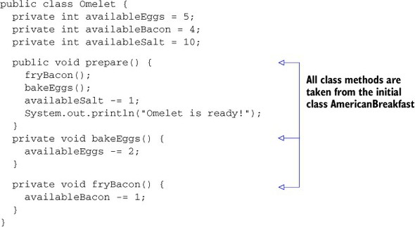
A new class, Omelet, has been introduced. It’s responsible for preparing the omelet, and all the methods and attributes needed to do so have been moved into it. AmericanBreakfast now has a reference to the Omelet class and invokes its prepare() method when needed (in the prepareOmelet() method). The rest of the code hasn’t been modified. Running a new SonarQube analysis after this refactoring yields LCOM4 scores of 1 for both classes. “But wait,” you might be saying, “Why doesn’t this still get a 2? The Omelet in AmericanBreakfast isn’t connected to availableOranges or availableSugar.” And of course, you’re right—because references to other objects (such as Omelet) don’t count. So AmericanBreakfast now only has one responsibility, to prepare the drinks.

Splitting a class is one way to address an inflated LCOM4 score, but LCOM4 isn’t the only reason you might need to refactor. Even if a class’s LCOM4 is perfect, its Response for Class (RFC) and the incoming/outgoing dependencies may still lead you to refactor.

6.3. RFC and couplings: classes with too many friends

We’ve looked so far at two types of complexity in a class: cyclomatic complexity and LCOM4. Now we’ll turn to the complexity of a class’s interactions with RFC and couplings. Only one of these two, RFC, has a dashboard widget available, so we’ll start with it.

RFC measures the size of a class’s response set, or how many distinct methods and constructors can be invoked by the class, including the class’s own methods and constructors (or the default constructor if there’s no explicit constructor for the class). RFC is another way of looking at complexity, but this time it’s about the complexity of a class’s interactions.

6.3.1. Response for Class

For any complexity-related metric, you want to keep the score low. That’s a given. But why keep this particular one low? Because having a class with a high RFC means that when you need to work on it, you have to understand a lot more than just the code in front of you to make sure your modifications are correct and appropriate. Conversely, a lower RFC means your maintenance job is easier. Having a high RFC also makes a class harder to understand when you’re considering reuse, harder to test, and less portable.

SonarQube presents RFC in a dashboard widget much like the one for LCOM4. We hope you added the RFC widget to the dashboard at the same time you added the LCOM4 widget. In that case, your dashboard now includes something like figure 6.8.

Figure 6.8. The RFC widget is one of the simplest, with only a distribution graph and an average score.

Again, you want to see the graph weighted to the left and the average RFC/class number low. How low? Well, there’s no best answer for that, except “as low as possible.” Acceptable RFC values vary from project to project, but in general, classes with an RFC of 40 or more need your attention. That’s because a high RFC means a method call to the class probably results in a large number of additional method calls either within the same class or to other classes (including superclass methods). In other words:

• It’s hard to understand, debug, and maintain it.
• You need to read several extra classes to unit-test it.
• Simple unit-test cases will end up with several mocked objects.
• A lot of effort is needed for even simple modifications.

Because there’s no perfect RFC score, you’ll notice slightly different behavior in the drilldown for RFC. From the dashboard, click-through on the RFC metric or graph, and you land at a drilldown—standard behavior. But the drilldown itself isn’t standard. Most drilldowns show only a subset of the files in a system: only the ones that need work. But the RFC drilldown shows them all, because there is no perfect score for RFC. Potentially, all the classes in a system need work. But aside from that minor point, the rest is pretty standard.

There’s no special tab for this metric, so choose a file and you’ll find yourself on the Source tab, as shown in figure 6.9. Once there, look at the numbers in the right column of the header, where you’ll see several design metrics, including Response for Class.

Figure 6.9. Various design metrics in the source code viewer tab

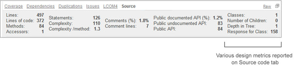
There’s not a lot else to see with regard to RFC. But before we move on to demonstrating the RFC calculation, we’d like to mention the other three metrics in this column: Classes, Number of Children, and Depth in Tree. They don’t have a dashboard widget, but they’re worth being aware of.

Classes reports on the total number of classes in the file. Typically it’s one, but if there are nested classes, they’re reflected here. Number of Children is how many classes inherit directly or indirectly from this class. Depth in Tree, sometimes called Depth of Inheritance Tree (DIT), is the converse: the level of inheritance from java.lang.Object. Because every class in Java inherits from java.lang.Object, 1—for something that extends Object directly—is the lowest number you’ll ever see for this metric. These metrics aren’t earth-shattering, but they’re worth a look when you’re considering the impacts of refactoring a class.

Now let’s revisit the refactored AmericanBreakfast class and compute its RFC.

Listing 6.7. AmericanBreakfast class

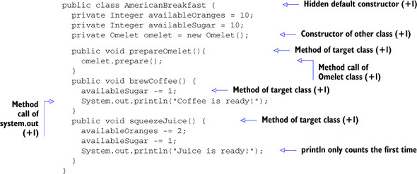
With three methods of its own, one member class, calls to the methods of two other classes, and the default constructor, AmericanOmelet has an RFC of 7. Notice that there are two instances in the code of System.out.println(), but the count is only incremented for it once, because each method is counted only once no matter how many times it’s used. So the second instance of System.out.println in listing 6.4 doesn’t count—literally!

What do you do if your RFC is too high? That depends on your situation and where the RFC hits come from. If it’s high because your class has a lot of methods, you may also find that its LCOM4 is high, and refactoring to break out some of those responsibilities into other classes will naturally help your RFC. The same thing applies if it’s high, because you’re making lots of calls to many other classes. That’s another case in which you may need to split the class into smaller, simpler classes with less going on. But if the RFC is high because you’re making a lot of calls to just one or two other classes, then you may need to examine whether the things happening in this high-RFC class belong in those other classes.

You’ve seen so far that cyclomatic complexity, LCOM, and RFC metrics are key metrics for refactoring decisions, but you should also take a class’s couplings into account. Next, we’ll look at couplings in depth, what they are and how to calculate them.

6.3.2. Couplings

Incoming (afferent) and outgoing (efferent) couplings are the last two metrics to consider when looking at the cohesion and stability of a class. Coupling is the academic term for dependency in software engineering. It’s used to describe the degree to which each component relies on or is relied on by other components.

These dependencies don’t have their own widgets, so you can’t get high-level information on them like you can with LCOM4 and RFC. As you’ll see, they’re only available at the file level via a dedicated tab in the file detail view, as shown in figure 6.10.

Figure 6.10. Afferent/efferent couplings of a class in the source code viewer

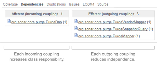
SonarQube shows couplings in two columns, with incoming couplings on the left and outgoing on the right. Notice that core Java classes (such as java.io.File and java.math.BigDecimal) don’t count for these metrics.

The afferent coupling (incoming dependency) count represents the number of other classes that depend on the target class. High scores mean the target class is playing an important role in the module/system, and it’s an indication of the importance of the tasks for which this class is responsible. High afferent coupling means a change to the target class will affect many other classes in the system (those that depend on it). So, changes to the class are riskier because there’s a higher chance of introducing new bugs in the calling classes, or even breaking an integration.

The efferent coupling (outgoing dependency count) is the number of classes that this class depends on. High values mean this class uses a lot of other classes, which could mean it’s brittle or unfocused, and definitely introduces the risk that every change to those other classes could affect this class’s behavior, usually negatively.

Like RFC, couplings are a reflection of the connectedness of a system. Even though couplings are a file-level metric, you can look at them as a reflection of the complexity of the whole package or module. Because complexity in general isn’t a good thing, you want to keep couplings low. The most popular way to reduce coupling is called decomposition. Extract smaller, more focused classes from the original, highly coupled classes so that the responsibilities of the initial class are spread among several simpler, easier-to-maintain classes with lower coupling.

Manually calculating the outgoing dependencies of a class is simple. Just count the class-level or method-level references to external classes.

Listing 6.8. AmericanBreakfast showing outgoing couplings

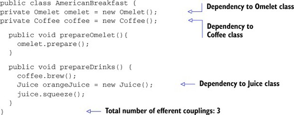
In listing 6.8, the AmericanBreakfast class has been modified slightly to better demonstrate how to find efferent couplings. There are now class-level dependencies to the Omelet and Coffee classes, and one method-level reference to the Juice class, for a total of three outgoing dependencies.

Trying to compute the incoming dependencies is a lot harder, because you would need to search all your code to find references to a given class. In large systems, and even in smaller ones, it would be time-consuming and error-prone or almost impossible to get those numbers on your own.

This concludes our tour of design metrics. As you’ve seen, SonarQube provides quite a few, some more important than others, but all worth at least a glance when you’re considering whether and how to refactor a class.

6.4. Summary

This chapter focused on file-level metrics related to design and complexity. Some of the concepts are considered hard to understand. But even if they’re top-of-mind for you, they’re still impractical to calculate by hand for an entire code base. Fortunately, SonarQube does the tedious bits for you and lays the numbers at your feet. In this chapter, you saw that

• High cyclomatic complexity makes your source code hard to understand and maintain. We’ve shown how SonarQube computes cyclomatic complexity and how to refactor for lower complexity.
• SonarQube’s LCOM4 presentation helps you find classes that do too much and shows you, at a file level, how a class’s responsibilities are grouped so you can make good refactoring decisions.
• RFC and the count of a class’s couplings help you understand a file’s interactions in your system. Social butterfly classes with a high RFC are invoking a lot of methods, either internally or externally, and may need to be reined in.

In this chapter, we looked at complexity at a file level. Before we move to part 2 of the book, we’ll talk about complexity at a package and system level and show you what SonarQube has to offer with regard to the architectural design of your system.