Chapter 9. Continuous Inspection with SonarQube

This chapter covers

• Understanding Continuous Inspection
• Triggering your analysis with Continuous Integration
• Monitoring quality evolution

With half the book behind you, you now have a thorough grounding in what SonarQube is telling you, including an in-depth understanding of the metrics behind the Seven Axes of Quality and a handle on how to tackle what those metrics show.

In this chapter we shift gears from theory to practice, with the introduction of Continuous Inspection, a practice that will boost your return on investment in SonarQube. So far, we’ve mentioned Continuous Integration (CI) a few times and hinted at its advantages. Now we’ll go in depth, starting with Continuous Inspection’s big picture and how SonarQube perfectly fits into a streamlined development process.

We’ll look at why it’s important to automate the Continuous Inspection practice and how easily that automation can be done. We’ll give you a step-by-step guide to integrating SonarQube with a CI system to automate your everyday analysis, and we’ll offer advice on best practices.

Once you’ve automated your analysis, you’ll want to dig in to some of SonarQube’s star features: differential views and version comparisons. In chapter 1, we touted SonarQube’s ability to help you see not just a project’s current state, but its quality evolution over time. Now it’s time to make good on that promise with differentials, which we believe to be one of SonarQube’s most valuable features. You’ll see how to check your projects’ progress—from day to day or version to version—and how to configure differentials to meet your needs.

9.1. Introducing Continuous Inspection

Google the term Continuous Inspection, and you’ll notice that several of the top results are related to SonarQube. What’s interesting is that although SonarQube dominates the CI, it’s not a concept that originated with SonarSource. It seems to have started in manufacturing, many years before SonarQube’s birth, and gradually taken root as a software concept. At the time, CI for software was something you had to cobble together yourself, laboriously adding to your build script each type of inspection you wanted (style, bugs, duplications, and so on). But of course SonarQube rolls all those inspections into one easy analysis, so it shouldn’t be surprising that in the last few years, SonarQube has been recognized as a must-have tool for CI.

But before we look at using SonarQube for CI, let’s examine some of the concepts behind it to help make the big picture clearer.

9.1.1. What and how?

First, “What should you inspect?” The answer seems pretty clear: an application’s source code. But what are you looking for? That’s where the Seven Axes of Quality—alternately referred to as a developer’s Seven Deadly Sins—come in. They represent developers’ most common bad habits (copy and paste, poor unit-testing, dirty code, and more). What you really want to do is keep an eye on what we covered in chapters 2 to 7.

With Continuous Inspection in place, you should easily be able to answer these questions:

• How much duplicate code was added last week?
• How well unit-tested are the files committed yesterday?
• Did we introduce any critical issues during the last iteration?

That might seem easier said than done, but with CI and SonarQube’s differentials, answering is easy.

To truly take advantage of a CI process, it should be a recurrent, automated activity that doesn’t steal more than a few minutes (if any!) from your day. Once you set it up, it should work without intervention, making fresh analysis results available on a regular basis, so that every morning you sit down to your cup of coffee and a fresh quality analysis. The only thing you’ll still need to handle is your coffee preparation. (Sorry, SonarQube’s not quite that good yet!)

Effectively implementing Continuous Inspection presupposes a regular build process—CI at best, but at least a nightly build. That’s what we’ll look at next.

9.1.2. Life before and after Continuous Inspection

To achieve Continuous Inspection, your best bet is to first implement a CI environment if you haven’t already. We’ll talk about your options in section 9.2. But first, let’s look at the advantages of CI.

In a traditional, pre-CI approach, developers check their changes in to the central source control management (SCM) system and get other developers’ checked-in changes—ideally, several times a day. Then, on occasion, the “build wizard” puts on her wizard hat to manually perform a build. In this environment, changes—and potential problems—can percolate for weeks or months before coming to the surface.

Add a CI tool, and your build (compile, run unit tests, deploy, and so forth) is triggered on a regular basis: automatically for every commit, or nightly if a build-per-commit seems like too much. Problems come to the surface quickly, and the build wizard can retire the funny hat.

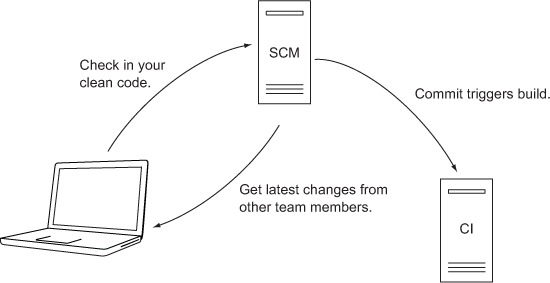
To accomplish this, configure your CI server to poll your SCM at predefined intervals (every few minutes, several times a day, and nightly are popular options), or set up event handlers in your SCM to fire off a build for each commit event—literally have the SCM push the commit event down to your CI system. Then instruct the CI tool to run all required build steps (compile, run tests, deploy, and so forth), and you’re done. Figure 9.1 shows what this system looks like.

Figure 9.1. Source code management with a CI server that pulls source code changes and triggers builds

Our experience has shown that moving from manual to automated builds can be a huge mental leap. If you aren’t familiar with CI practices, then you’re probably shocked by the thought that your system would be built multiple times a day by a ... machine. But consider the advantages. First, you minimize the time it takes to create your application’s executable. In fact, you don’t spend any time at all on it. It happens regularly and automatically, which means you always have the latest ready-to-ship build for testing, sales presentations, or beta evaluation. All unit tests are executed each time you build your system; and if something goes wrong, all team members are immediately notified. No more dark arts to make sure everyone has committed all their changes. You configure your build job once, and CI knows when to trigger it.

Once CI is set up and humming, it’s time to invite SonarQube to join the game. SonarQube integrates easily into most CI setups. You need to follow only two steps:

1.  Decide how often you’d like to analyze your project.

2.  Create a CI job that runs the analysis.

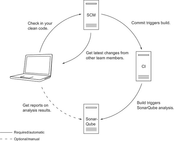
Figure 9.2 shows the system when you’re finished. What you see is a basic CI workflow. As illustrated, SonarQube is triggered automatically by build jobs on the CI server. When the analysis is complete, developers and other team members can get the latest quality reports without worrying about manually triggering the analysis—in essence, their check-ins did that for them.

Figure 9.2. Source code management with CI server and SonarQube. Build automatically triggers SonarQube analysis.

Now you have an idea of the details. Use CI tools to build your code base automatically, and you can take advantage of that automation to add Continuous Inspection to your system. But let’s back up and look at why you’d want to.

9.1.3. The big picture

CI addresses a unique challenge: to help you and your team track and reduce your project’s technical debt on an ongoing basis.

Financially speaking, debt is an obligation of a creditor to the debtor. For instance, when you take a loan from a bank, you’re committed to make a monthly payment until you cover the original amount plus the accrued interest. Usually, the loan is repaid in a fixed period of time. Miss a payment, and the total amount you owe—the debt—increases due to additional interest (and fees); thus you need more money to meet your obligation.

Similar principles apply to technical debt. The difference is that there is no initial obligation. The debt starts to build when the first commit takes place, and it’s increased every time you add new code to the project. It’s like when you get a new credit card. On the first day, the balance is zero, but every purchase (commit) is a charge to your card (technical debt) that eventually you’ll have to repay.

But who is responsible for increasing your technical debt? Every duplicated line, every new issue, and every file not covered by unit tests adds to your technical debt. If you don’t take action to pay it down, your technical debt will grow quickly and eventually cost you much more effort—and money—later in the project.

Technical debt comes in three flavors. As you can see, there is a straightforward relationship between the types of technical debt and the Seven Axes of Quality:

• Code— Issues, duplications, and absence of commenting and documentation
• Design— Poor design, increased complexity, low cohesion and high coupling, and architectural problems
• Testing— Low or no unit-test/integration-test coverage, and tests that are hard to maintain

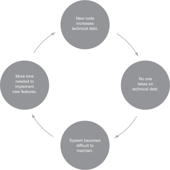
There are plenty of reasons to make charges against your credit card, just as there are plenty of reasons why technical debt is added. And like paying your monthly credit card bill, you know you should pay down your technical debt regularly. But there’s always the temptation to avoid dealing with it: “Paying down technical debt will reduce productivity and leave less time for new features.” In the short term, that may be true; but by ignoring your debt, you’ll end up in a vicious cycle. As shown in figure 9.3, the longer you avoid paying your technical debt, the harder it will be to maintain your system, sending your productivity into a downward spiral.

Figure 9.3. Not paying down technical debt will make your system hard to maintain and will eventually decrease productivity.

There is only one way to eliminate this deadlock: pay down your technical debt continuously during the project’s lifetime. Make this your goal, and you’ll find SonarQube an invaluable tool for reaching it. The rest of this chapter shows you how. We’ll start by automating SonarQube analysis with a CI server and then show you how to track changes across time using differential views.

9.2. Triggering your analysis with CI

There are lots of CI servers out there—a dizzying array—but direct CI/SonarQube integration is available for only a few: Jenkins and AnthillPro, both of which are free and open source; and Atlassian Bamboo, a commercial offering. In this section, we’ll look at the direct integration of Jenkins in depth and Atlassian Bamboo briefly.

Note

Even servers that don’t have direct integration can still be used to trigger SonarQube analyses. It’s a matter of firing the proper command after the build. The SonarQubeSource documentation offers advice at http://mng.bz/43GI for doing that for three other popular servers: Apache Continuum, CruiseControl, and JetBrains TeamCity. Even if your CI server isn’t one of those three, the advice you’ll find at this site may be helpful.

If your team doesn’t currently have a CI server, you’ll need to pick one and set it up. Our favorite is Jenkins. Unfortunately, we don’t have room here to show you how to get it up and running, but the Jenkins community documentation can guide you (http://jenkins-ci.org/). Like some of the other tools we’ve mentioned (and like SonarQube itself), Jenkins is free, open source, and dependable. Plus, paid support is available if you want it. It’s also the most popular open source CI tool because it can be used with any programming language; and, last but not least, it’s easy to set up even without previous experience.

From this point on, we’ll assume you have a CI server up and running. The next step is to set up a CI job. We’ll use Jenkins in our examples because, as we’ve mentioned, it’s a favorite—not just with us but generally. Basic knowledge of managing Jenkins jobs isn’t required for this section, but it will help you better understand what we’ll tell you.

9.2.1. Jenkins setup

The procedure to integrate SonarQube with Jenkins is straightforward. It consists of the following tasks in Jenkins:

1.  Install the SonarQube Jenkins plugin.

2.  Configure your SonarQube installation.

3.  Configure SonarQube Runner.

4.  Configure a job that triggers a SonarQube analysis. (If you’re dealing with a Java or C# project, also make sure the job performs a build.)

Next, we’ll look at each of these steps in detail.

Installing the Jenkins plugin

Before you start, double-check that both your SonarQube instance and your Jenkins server are up and running, because you’ll need them during installation. Then, install SonarQube’s Jenkins plugin.

This can be easily done from the Jenkins update center. Point your browser to the following URL: http://[yourJenkinsServer]:8080/pluginManager/available (if you changed the port of the CI server, change the URL accordingly), or use the Jenkins UI’s navigation by choosing Manage Jenkins in the left rail menu and then Manage Plugins. Finally, click the Available tab to get a list of all available plugins. On this tab, you can use the search filter at upper right to quickly filter Jenkins’ long list of plugins, as shown in figure 9.4.

Figure 9.4. Installing SonarQube plugin through Jenkins’ update center

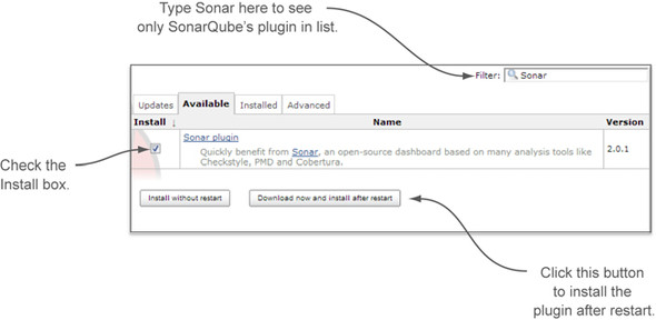
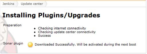
Select the Install check box, and click Download Now and Install After Restart. (You could click Install Without Restart, but the restart doesn’t work properly on some platforms.) When Jenkins finishes downloading the plugin, you see a message similar to what’s shown in figure 9.5. Restart your Jenkins installation to activate the plugin and proceed with the configuration.

Figure 9.5. When the plugin is downloaded, you’re notified.

Setting up your SonarQube installation in Jenkins

With the plugin installed, you’re ready to configure it with some server-level settings. Start by choosing the Manage Jenkins link in the left rail. Then choose Configure System, and find the SonarQube section on the page. It will probably be toward the bottom. Figure 9.6 shows what you’re looking for.

Figure 9.6. Adding a new SonarQube installation in Jenkins

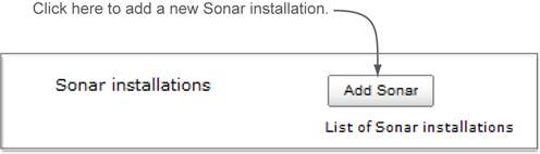
You need to tell Jenkins about your SonarQube installation. Click the Add Sonar button to add a few fields and some buttons to the page. Then click the Advanced button, and you’ll see a slew of additional fields as shown in figure 9.7. It’s time to fill them in.

Figure 9.7. The SonarQube plugin’s available configuration options

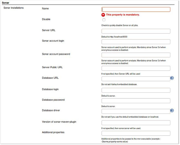
First, give your SonarQube install a name. Skip the Disable field for now—it disables SonarQube for all jobs, no matter what. If Jenkins and SonarQube are running on the same machine, and you haven’t changed SonarQube’s default port (9000), then you can skip the next two properties (Server URL and Server Public URL). If not, enter the proper values in these fields.

Next you need to set up your database connection and configuration. Click the Help icon (the question mark) next to the Database URL input text to see some URL examples.

After that, enter the credentials you selected when you created SonarQube’s database user (see appendix A for detailed instructions on installing and configuring SonarQube). Finally, enter the database driver. Again, the Help icon will give you examples for the most popular databases. Leave the last two properties empty.

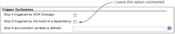
Now proceed to the triggering configuration. Figure 9.8 shows the available options. We suggest that you leave all of them unchecked, because the setup we’ll recommend later will require the analysis to be triggered by SCM changes.

Figure 9.8. SonarQube plugin: available triggering configuration options

To finish the SonarQube plugin configuration, click the Apply button, not Save. If you do click Save, return to the configuration page—you’re only half done. Next you need to configure Jenkins’ SonarQube Runner.

Configuring SonarQube Runner in Jenkins

Find the SonarQube Runner section on the page, and click the Add Sonar Runner button. As figure 9.9 shows, doing so again adds options to the page.

Figure 9.9. Setting up a SonarQube Runner installation is easy. Click the Add button, name the installation, and choose Install Automatically.

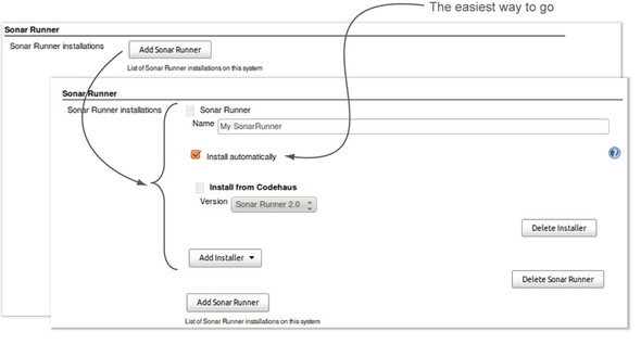
Give your installation a name; because it’s possible to have multiple instances of SonarQube Runner installed on a Jenkins server, this will help you tell them apart. Then, assuming you’re after the easiest route, select Install Automatically, and you’re finished. Click Save.

Now you’re ready to configure your job to run an analysis.

Enabling SonarQube analysis in a build job

Create a new job (you’ll land automatically at its configuration page), or navigate to the configuration page for the existing job that you’d like to use for analysis. Whether you choose an existing job or set one up from scratch, make sure it includes a step to compile your code if you’re dealing with Java or C#, because SonarQube performs byte-code analysis for both languages.

Now you’re ready to enable SonarQube in your job, but there are two ways to do that, as figure 9.10 shows. First you’ll have to figure out which one to use.

Figure 9.10. SonarQube analysis is available as either a build step or a post-build action, but the only time you want to use the post-build option is for Maven projects.

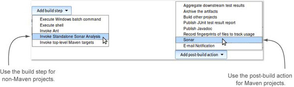
The first option lets you trigger a SonarQube analysis as a build step. Unless you’re in a Maven shop, this is the one you’ll use. The second option is a post-build action, and it’s only appropriate for Maven projects. It’s available for all Jenkins jobs, even for non-Maven projects; but if you use it on a non-Maven project, your build will always fail (because you don’t have the right prerequisites in place). We’ll look first at the build step option, which is shown in figure 9.11.

Figure 9.11. Configuring standalone SonarQube Runner properties

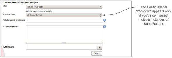
If you have multiple JDKs configured in Jenkins, the JDK drop-down menu lets you choose among them. Similarly, if you have multiple instances of SonarQube Runner configured, you’ll see a Sonar Runner drop-down menu (it disappears if you have only one SonarQube Runner instance). The next two inputs present an either/or proposition. If your project’s workspace includes a sonar-runner.properties file (whether it goes by that name or not), provide its path—relative from the project root—in Path to Project Properties. Otherwise, use the Project Properties field to enumerate your project’s analysis properties. The final input, JVM Options, isn’t typically needed, but it gives you the ability to pass additional JVM arguments to the analysis just in case.

You’re done at this point. But before you click Save, be sure your SonarQube build step comes after your job’s compile step (you can drag/drop steps to reorder them).

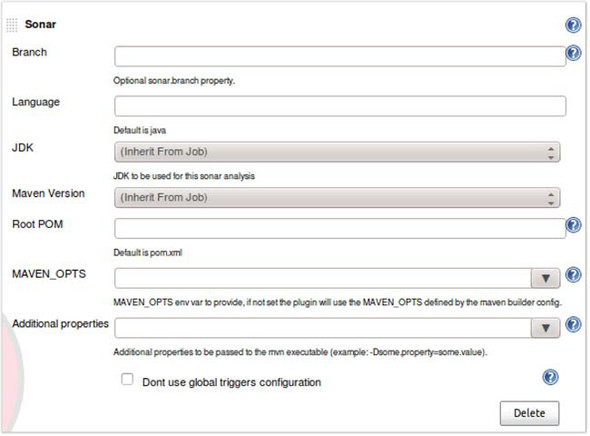
The Maven-only, post-build option can be turned on by picking SonarQube from the Add Post-Build Action menu. This gets you an all-defaults analysis. But if you need more flexibility, clicking the Advanced button presents a host of options, as shown in figure 9.12.

Figure 9.12. Advanced configuration for a SonarQube post-build action

Tip

It’s always a good idea to click the Advanced button whenever you see it in Jenkins. Many interesting things may be hidden underneath, and the fact that it’s not expanded by default doesn’t mean none of the values are filled in.

SonarQube uses the Branch and Language properties to specify a SCM branch or a language other than Java. If you need more information about these properties, jump to appendix B, which is about running and configuring a SonarQube analysis. The Root POM field lets you specify where to find your pom file if it’s not in the standard spot. The MAVEN_OPTS input lets you pass additional options into Maven for the analysis, such as -X to show debug logging. The Additional Properties field lets you define any additional properties that may be needed for the analysis. A valid input string looks something like this:

-Pintegration-tests -Dappserver=tomcat -Ddatabase=mysql

Finally, you can override the global triggering configuration (those check boxes we told you to skip in the server-level configuration) by selecting the relevant option and adjusting the settings to fit your project needs.

Whichever route you use to configure your analysis, when you’re done with the configuration, be sure to click Save or Apply. The next time your job runs, you’ll see in the console log that after Jenkins completes the build (your job does contain a compile/build, right?), a new SonarQube analysis is triggered with the parameters you configured.

We’ve covered everything you need to know to integrate your Jenkins installation with SonarQube, and you’ve seen how to enable quality analysis in build jobs. Next we’ll give you an overview of SonarQube integration with other popular CI servers.

9.2.2. Other CI systems

In general, there are no plugins for other CI servers. The fact that Jenkins is dominant has stopped development efforts on most other fronts—with one exception.

Marvelution (https://marvelution.atlassian.net) offers a stable open source plugin (https://marvelution.atlassian.net/browse/BAMSON) to integrate SonarQube with the Bamboo CI server. Bamboo is a popular commercial CI and release-management system. It’s developed by Atlassian (www.atlassian.com/software/bamboo) with lots of features and great integration with other Atlassian products such as JIRA and Confluence. Marvelution’s web site offers user administration guides; so if you’re already using Bamboo, take a serious look at the Marvelution plugin and open the door to the advantages of Continuous Inspection with SonarQube.

9.2.3. Best practices

So far, we’ve shown you how to automate your SonarQube analysis through a CI environment. But we think the puzzle is missing a piece. Usually, CI builds are triggered after every change of the source control files or at predefined time intervals (every few minutes or a couple times a day).

Because it’s fair to assume that a programmer normally commits small code changes 3 or 4 times a day, on a medium-sized project with 5 developers that means the CI server builds the system 15 to 20 times a day. You do want your SonarQube analysis to run regularly, but 20 times a day is too often. Analyzing after each commit is overkill because frequent, small commits mean there are few changes in the source code and the analysis results may not change. For one thing, there’s the system load consideration. The cycles required to run an analysis are usually well worth it, but it does take a while to run an analysis; and if it isn’t going to show you anything new, why not save those resources?

Plus, you’ll see when we look at differentials in the next section that running an analysis that you know isn’t likely to include any changes is counterproductive.

So how often you should run SonarQube? Remember the following rule:

Analyze once or twice a day but only if there are changes in the source control repository.

Following this rule is easier than it may seem. For projects that build on a CI basis—after every commit—you split the analysis job off from the build job and run it nightly. (Okay, it isn’t truly Continuous Inspection, but regular or perhaps continual inspection. Even if we have to waffle on the words, it’s still incredibly valuable.) For projects that only build on a nightly basis—or a couple times a day at most—you integrate analysis into the main build job. Then Jenkins makes it easy to trigger the job (set it up to run) only when your cronned poll of the SCM indicates code changes.

Because we’ve told you to be choosy about when you analyze, you may be wondering whether you should restrict what you analyze. Should you include integration, acceptance, or performance tests? Should you analyze only the main language of your project, or all of them? Again, the answer’s simple: make your analysis as broad as you can.

As an example, consider a typical JEE web application. The persistence layer, the business logic, and part of the user interaction logic are written in Java. The web interface may be developed with JSF pages using XHTML templates and plenty of JavaScript. Plus several modules include XML processing. So there are four different kinds of source to analyze.

If each language is segregated into a different module of a multimodule project, then you’re in luck: SonarQube handles this automatically. But even if the lines in your project aren’t so cleanly drawn, you can still handle this easily. Set up a separate build step for each language (if it’s a Maven project, use the post-build action for the main language and build steps for the rest). Make sure you set the language property appropriately for each run and differentiate the runs by either using the branch property or setting a different project ID for each one.

Once you’ve finished configuring your build jobs, your SonarQube analysis should be fully automated. You’ll have good, fresh data rolling in all the time. Now we’ll move on to differentials, which help you take full advantage of your regular analysis by letting you easily compare the current state to a previous analysis.

9.3. Monitoring quality evolution

Let’s say you’ve presented SonarQube to your boss and she’s excited about it. Now she wants you to measure the test coverage of a critical system for the next couple months and verify that it’s trending in the right direction.

You’re thrilled that she’s buying in, so you scoot back to your desk to check the project dashboard. Great Scott! Last night’s CI analysis shows that your project is more than 75% covered by tests! Thrilled, you make a note of the number and head out to lunch.

A few days later, you check the dashboard again. Testing coverage is around 72%. You’re glad to see it so high, but you can’t find the note with the previous number, so you can’t tell your boss if coverage is increasing or not. This time you’ll be sure to put the note in a more secure place.

Fortunately, there’s a better way: SonarQube’s differential views.

9.3.1. Exploring differential views in the project dashboard

To start working with differential views, go to the dashboard of a project you’ve analyzed at least twice (preferably on two different days). At the top of the screen is the Differential drop-down menu, as shown in figure 9.13.

Figure 9.13. The Differential drop-down menu in the project’s dashboard

If you’re following along on your own instance of SonarQube, you’ve probably noticed that the options in your drop-down menu are different than what’s shown in figure 9.13. And that’s the power of this service. You can fully customize what you see in the drop-down menu at the global and project levels. We’ll show you how in a minute, but first let’s see what happens when you select a value in the drop-down list. Try picking the first option, which should be Δ Since Previous Analysis (Some date), and notice how the widgets change when the page reloads, as shown in figure 9.14.

Figure 9.14. Picking an option from the Differential drop-down list changes the widgets.

Note

The reports you see when you select a period, say Δ Over 5 days, don’t change dynamically. Go a few days without analyzing, and what you’re looking at will be the change over eight days—that is, five-day results that are three days stale. You’ll need to analyze each day to see different numbers day by day.

If you take a closer look at the dashboard you’ll notice that all the trending arrows have been replaced by colored (red, green, or black) numbers in parentheses. Furthermore, two widgets (issues and unit-testing coverage) have been enriched with new metrics. Let’s examine them step by step.

The meaning of colored numbers

At the right of each metric is a number showing the difference between the latest analysis and the snapshot analysis you selected in the Differential drop-down menu. We’ve said before that SonarQube uses colored trend arrows—green for good and red for bad. When you’re in differential mode, the same applies to the numbers that replace the trend arrows. Good changes are green, bad are red, and value-neutral are black.

Look at the comments and duplications widget in figure 9.15. In this case, the density of comments has decreased from 7.0% to 6.9%, so in SonarQube, the difference is colored red. Similarly, there are 33 new duplicated lines and 3 new duplicated blocks of code. They negatively affect the quality of the project, so they’re shown in red.

Figure 9.15. Colored numbers indicate improvement, deterioration, or no impact on quality analysis.

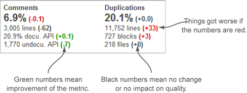
On the other hand, two of the documentation metrics have improved, so their Δ values are shown in green. Looking at your own dashboard, you’ll see that color has nothing to do with whether the value of the change is a negative or positive number—it’s all about whether the metric is improving or deteriorating. This means metrics with no change and metrics that don’t affect the quality of the project, such as duplications files and lines of comments in our example, are shown in black.

New metrics in the unit-testing widget

In addition to using the same red/green coloring for differential values, the unit-testing widget adds metrics in differential mode. But to activate the feature, you need to install and configure the SCM Activity plugin we discussed in chapter 2.

Once you’ve done that, differential mode adds a new section to the lower left of the unit-testing widget, as shown in figure 9.16. It’s titled On New Code, and it shows the three coverage metrics for code added in the comparison period.

Figure 9.16. Unit-testing widget when a differential view is enabled

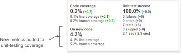
Our experience has shown that monitoring this section regularly and politely nagging developers who’ve checked in fresh and untested code keep an application’s overall code coverage at the highest levels. In other words, Continuous Inspection (and correction) works!

New metrics in the issues widget

The issues widget also adds metrics in differential mode. Just below the total number of issues, you can see how many issues were added and removed in the comparison period, as shown in figure 9.17.

Figure 9.17. The rules compliance (issues) widget when a differential view is enabled

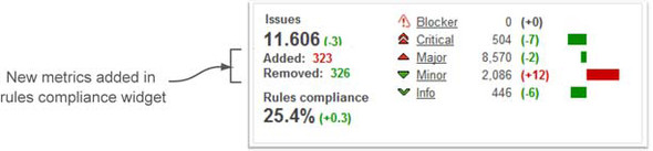
Look again at the differential numbers, and you may notice that the differential values on the right (for Blockers, Criticals, and so on) don’t add up to the Added and Removed values on the left. That’s because the numbers on the right are net changes and the ones on the left are gross values. But sum each set, and the numbers should match: (323 -326) = (-7 -2 +12 -6) = -3.

So far, we’ve looked at differentials on the dashboard, but they extend into some drilldowns as well. Next, we’ll drill into issues while in differential mode.

9.3.2. Differential views in the issues drilldown

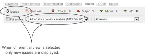
The issues drilldown you saw in chapter 2 had a few extra features compared to other drilldowns: severity and rule lists. It offers one more plus by honoring differentials too, letting you examine how many issues for each severity, rule, and so on have been added in a differential period, as shown in figure 9.18.

Figure 9.18. Issues widget when a differential view is enabled

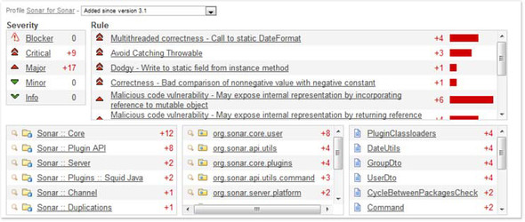
Only new issues are shown here; existing issues are omitted. And don’t look for any green in this differential view—it only shows added issues, not issues that were removed.

9.3.3. Differential views in the source code viewer

Click any filename to reach the Issues tab of file detail view. When you do so in differential mode, the header changes slightly, again to show only new issues, as shown in figure 9.19. This feature is available only when you have the SCM Activity plugin installed and enabled for the current project.

Figure 9.19. The Issues tab in the source code viewer shows only new issues when a differential view is selected.

To decide which issues to show in differential mode, SonarQube applies an algorithm.

If there was an issue with the same rule, then it checks for the following:

• The issues have the same line number.
• The issues have the same line hash.
• The issues have the same message.

If at least two conditions are true, the issue is considered old; otherwise it’s marked as new and displayed in the differential drilldown. As we’ve hinted, differentials aren’t available on all tabs—just Issues, Coverage, and Source. Yes, you can use differentials to see which lines of code have been added in the comparison period!

9.3.4. Choosing differential periods

When we first showed you the differential drop-down menu, it held some values that probably don’t match what’s in your drop-down menu. For starters, our drop-down menu had five periods and yours probably has three, if it’s a new SonarQube installation. Plus, some of our periods were different than yours. Well, now it’s time to talk about those differences. As you’ve seen, you can put up to five values in the drop-down menu. Chapters 14 and 15 will show you how to change those values. Here we’ll talk about what you might want to change them to.

The first three are set at the global level and will be the same for all projects, unless you explicitly override them at the project level. By default, the three global periods point to the previous analysis, 5 days ago, and 30 days ago. At the project level, you can add two more periods for each project. The periods are named (not surprisingly) Period1 through Period5.

SonarQube offers the following ways to define a threshold period:

• Use the string “previous_analysis” to compare the latest analysis with previous one.
• Set an integer number of days before the current analysis. Note that this can yield approximate results. SonarQube finds the first available snapshot analysis inside the date range. So if there’s not a snapshot that’s exactly five days old, you’ll get a comparison against a four-day-old or three-day-old snapshot.
• Predefine a date in yyyy-MM-dd format. SonarQube finds the first available snapshot analysis in the date range.
• Use the string “previous_version” to compare the latest analysis with the previous project version (corresponding to the last time you changed your project’s sonar.projectVersion analysis property).

There is no “right” definition for these periods, but here are some tips based on our experience:

• Keep “previous_analysis” as the first period.
• Decide how frequently you’ll inspect your analysis results, and define corresponding periods by specifying numbers of days. For instance, we bump the default 5-day period up to 7 days so we can check week over week; and a 30-day period would give you a month-over-month comparison.
• Define a “previous_version” threshold, either on a global or (preferably) a project level.

Earlier we said that you could set your differential periods to specific dates, but we warned that you’d want to read up on events first (see chapter 15). That’s because any snapshot that doesn’t have an event flagged against it is subject to being deleted during housekeeping. If you do decide to set your differentials to dates—say January 1 each year—you’ll want to not only run a starting-point analysis that day but also make sure those analyses are marked with events. Because you can set version or other events retroactively through SonarQube’s interface, they’re probably the best options to use.

Once you make your changes, the drop-down menu text changes immediately to reflect them, but remember that under the covers, those text values still correspond to Period1, Period2, and so on. This means that if you adjust Period2 to be seven days instead of five and immediately check your dashboard to see the seven-day differential, you’ll be disappointed. Differential modes look dynamic, but they’re not. So you won’t see a seven-day differential until after your next analysis.

But there is a way to satisfy—at least partially—the immediate urge to see the difference between one version of an application and another. And that’s next.

9.3.5. The Compare service

Filed under the Tools menu in the left rail, you’ll find Compare. It appears at both the global and project levels and leads to an interface that allows you to put the metrics for specific project versions side by side for comparison. Access it from the project level, and it’s automatically populated with up to six of that project’s most recent versions, as shown in figure 9.20.

Figure 9.20. The Compare tool lets you compare selected metrics from multiple versions—of the same project or different ones!

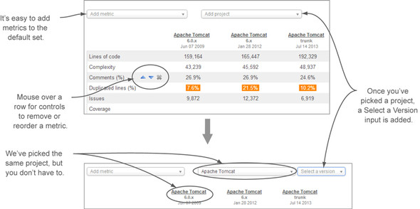
The Compare service doesn’t do the math for you, like differentials, so you have to figure out for yourself whether code coverage increased or decreased from version to version. But unlike differentials, it lets you do ad hoc comparisons on a whim—in a project or across multiple projects.

By default, Compare shows a basic set of metrics, but you can easily add metrics to or remove them from the list. You can also easily reorder both the metrics and the projects—just mouse over the labels to reveal those controls.

At this point, you’ve plumbed the depths of Continuous Inspection and quality-evolution monitoring through differentials and version comparisons. Now we’ll close the chapter, as we usually do, with an overview of related plugins.

9.4. Related plugins

A couple of plugins related to CI and inspection offer related metrics and utilities. Let’s look at the advantages of adding them to your process.

9.4.1. Cutoff

Have you ever wanted quality reports on just the code changes made last month? Unless you happen to have tagged your repository a month ago, it seems like an impossible task. Try to figure it out manually and you’d need weeks.

And that’s where the Cutoff plugin comes in. At both the global and project levels, it lets you define either a specific date, like 1/1/2013, or a cutoff period, such as 60 days, and it tells SonarQube to ignore files that haven’t been touched since then. It’s especially useful for teams that maintain legacy systems and want to focus only on their own changes—not what was written years ago by long-gone developers. It lets them define the date they picked up maintaining the system, and it narrows SonarQube’s reporting to just the files they’re interested in.

You need to be aware of a couple of things with this plugin. If both the date and period are defined, the period is ignored in favor of the date. Also, it relies on the system date. So, double-check that your system date is correctly set before you run a new analysis with a date threshold. Furthermore, checking in minor changes to an “old” file resets its date, meaning that all its legacy issues are included to your “only new” analysis.

9.4.2. Build Breaker

The Build Breaker plugin is a simple yet useful plugin with a sole purpose: to break the CI build when new alerts are raised during an analysis.

We haven’t spent a lot of time yet on alerts, but the basic concept is that you can define warning and error thresholds on specific metrics. When a project’s value crosses the threshold, SonarQube raises an alert, and the Build Breaker plugin lets you take advantage of your CI server’s notification mechanisms to raise a hue and cry. That means you need to set some alerts (covered in chapter 13) to take full advantage of this plugin.

As an example, assume that you want to be notified if your duplications rise over 2%. All you have to do is to install this plugin and create an alert in the project’s quality profile. Then, if your threshold is hit during an analysis, the Build Breaker plugin returns an error status to the CI server, and the build is marked as failed, as shown in figure 9.21.

Figure 9.21. CI log output when analyzing SonarQube with the Build Breaker plugin enabled

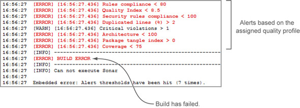
The beauty of this integration is that, assuming you’ve configured your CI server to send notifications (emails, instant messages, and so on) for build failures, whenever an alert is raised on the SonarQube side, all team members are automatically notified by the CI engine, eliminating the need for manually visiting SonarQube to check for new alerts. Even better, because this plugin is installed on the SonarQube side rather than in your CI server, it can be used with any CI server that respects a subprocess’s return code.

9.5. Summary

This chapter was a real workout! First we looked at why CI and Continuous Inspection should play an important role in your development process. You saw that automating your project analysis is the basic foundation to apply Continuous Inspection.

Thanks to some free plugins, SonarQube smoothly cooperates with the most popular CI servers: Jenkins, AnthillPro, and Bamboo. You saw how to install and configure SonarQube integration for Jenkins and how to trigger analysis in a build job—including multiple languages. Best practices say that you’ll set this up in a job that only runs once a day or so.

But there’s no real Continuous Inspection if you can’t monitor specifically how your source code quality is changing, so next we looked at SonarQube’s differentials, which give you details on the changes since a given point in time. Differential views, which are fully customizable on both the global and project levels, allow you to compare the current quality status with predefined thresholds—up to five of them—such as the latest build, latest version, or a custom date. All SonarQube’s core widgets take advantage of this service by showing the differences between the current analysis and the selected period. Further, a couple of them (issues and unit testing) even add new metrics in differential mode.

You also saw the Compare tool, which gives you the ability to compare any two project versions (even any two projects) on an ad hoc basis. Good differentials require a little planning, but you can run the comparison tool on a whim.

Closing this chapter, we showed you some plugins that either extend the differential views feature (Cutoff) or improve integration with CI servers (Build Breaker).

Now you know how to continuously track what’s going right—or wrong—in your project. In the next chapter, we’ll look at the tools SonarQube offers to help you manage your code reviews.