
7Superhedging
The idea of superhedging is to find a self-financing trading strategy with minimal initial investment which covers any possible future obligation resulting from the sale of a contingent claim. If the contingent claim is not attainable, the proof of the existence of such a “superhedging strategy” requires new techniques, and in particular a new uniform version of the Doob decomposition. We will develop this theory for general American contingent claims. In doing so, we will also obtain new results for European contingent claims. In the first three sections of this chapter, we assume that our market model is arbitrage-free or, equivalently, that the set of equivalent martingale measures satisfies
In the final Section 7.4, we discuss liquid options in a setting where no probabilistic model is fixed a priori. Such options may be used for the construction of specific martingale measures, and also for the purpose of hedging illiquid exotic derivatives.
7.1 P-supermartingales
In this section, H denotes a discounted American claim with
Our aim in this chapter is to find the minimal amount of capital Ut that will be needed at time t in order to purchase a self-financing trading strategy whose value process satisfies Vu ≥ Hu for all u ≥ t. In analogy to our derivation of the recursive scheme (6.5), we will now heuristically derive a formula for Ut. At time T, the minimal amount needed is clearly given by
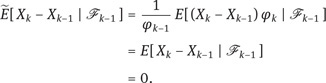
At time T − 1, a first requirement is to have UT−1 ≥ H T−1. Moreover, the amount UT−1 must suffice to purchase an FT−1-measurable portfolio ![]() T such that
T such that ![]() T · XT ≥ HT almost surely. An informal application of Theorem 1.32, conditional on FT−1, shows that
T · XT ≥ HT almost surely. An informal application of Theorem 1.32, conditional on FT−1, shows that
Hence, the minimal amount UT−1 is equal to the maximum of H T−1 and this essential supremum. An iteration of this argument yields the recursive scheme
for t = T −1, . . . , 0. By combining Proposition 6.43 and Theorem 6.51, we can identify U as the upper Snell envelope
of H with respect to the stable set P, where UP∗ denotes the Snell envelope of H with respect to P∗. In the first three sections of this chapter, we will in particular give a rigorous version of the heuristic argument above.
Note first that condition (7.1) implies that
where we have used the identification of the upper bound πsup(H) of the arbitrage-free prices of H given in Theorem 6.31. It will turn out that the following definition applies to the upper Snell envelope if we choose Q = P.
Definition 7.1. Suppose that Q is a nonempty set of probability measures on (Ω,FT). An adapted process is called a Q-supermartingale if it is a supermartingale with respect to each Q ∈ Q. Analogously, we define the notions of a Q-submartingale and of a Q-martingale.
◊
In Theorem 5.25, we have already encountered an example of a P-martingale, namely the value process of the replicating strategy of an attainable discounted European claim.
Theorem 7.2. The upper Snell envelope U↑ of H is the smallest P-supermartingale that dominates H.
Proof. For each P∗ ∈ P the recursive scheme (6.33) implies that P∗-a.s.
Since ![]() is a finite constant due to our integrability assumption (7.1), induction on t shows that
is a finite constant due to our integrability assumption (7.1), induction on t shows that ![]() is integrable with respect to each P∗ ∈ P and hence is a P-supermartingale dominating H.
is integrable with respect to each P∗ ∈ P and hence is a P-supermartingale dominating H.
If ![]() is another P-supermartingale which dominates H, then
is another P-supermartingale which dominates H, then ![]() Moreover, if
Moreover, if ![]() for some t, then
for some t, then
Thus,
and backward induction shows that ![]() dominates U↑.
dominates U↑.
For European claims, Theorem 7.2 takes the following form.
Corollary 7.3. Let H E be a discounted European claim such that
Then
is the smallest P-supermartingale whose terminal value dominates HE.
Remark 7.4. Note that the proof of Theorem 7.2 did not use any special properties of the set P. Thus, if Qis an arbitrary set of equivalent probability measures, the process U defined by the recursion
is the smallest Q-supermartingale dominating the adapted process H.
◊
7.2Uniform Doob decomposition
The aim of this section is to give a complete characterization of all nonnegative P-supermartingales. It will turn out that an integrable and nonnegative process U is a P-supermartingale if and only if it can be written as the difference of a P-martingale N and an increasing adapted process B satisfying B0 = 0. This decomposition may be viewed as a uniform version of the Doob decomposition since it involves simultaneously the whole class P. It will turn out that the P-martingale N has a special structure: It can be written as a “stochastic integral” of the underlying process X, which defines the class P. On the other hand, the increasing process B is only adapted, not predictable as in the Doob decomposition with respect to a single measure.
Theorem 7.5. For an adapted, nonnegative process U, the following two statements are equivalent.
(a) U is a P-supermartingale.
(b) There exists an adapted increasing process B with B0 = 0 and a d-dimensional predictable process ξ such that
Proof. First, we prove the easier implication (b)⇒(a). Fix P∗ ∈ P and note that
Hence, V is a P-martingale by Theorem 5.14. It follows that Ut ∈ L1(P∗) for all t. Moreover, for P∗ ∈ P
and so U is a P-supermartingale.
The proof of the implication (a)⇒(b) is similar to the proof of Theorem 5.32. We must show that for any given t ∈ {1, . . . , T}, there exist ξt ∈ L0(Ω,Ft−1, P;ℝd) and ![]() such that
such that
This condition can be written as
where Kt is as in (5.12). There is no loss of generality in assuming that P is itself a martingale measure. In this case, Ut − Ut−1 is contained in L1(Ω,Ft , P) by the definition of a P-supermartingale. Assume that
Absence of arbitrage and Lemma 1.68 imply that C is closed in L1(Ω,Ft , P). Hence, Theorem A.60 implies the existence of some Z ∈ L∞(Ω,Ft , P) such that
In fact, we have α = 0 since C is a cone containing the constant function 0. Lemma 1.58 implies that such a random variable Z must be nonnegative and must satisfy
In fact, we can always modify Z such that it is bounded from below by some ε > 0 and still satisfies (7.2). To see this, note first that every W ∈ C is dominated by a term of the form ξt · (Xt − X t−1). Hence, our assumption P ∈ P, the integrability of W, and an application of Fatou’s lemma yield that
Thus, ifwe let Zε := ε+Z, then Zε also satisfies E[ Zε W ]≤ 0 for all W ∈ C . Ifwe chose ε small enough, then E[ Zε (Ut −Ut−1) ] is still larger than 0; i.e., Zε also satisfies (7.2) and in turn (7.3). Therefore, we may assume from now on that our Z with (7.2) is bounded from below by some constant ε > 0.
Let
and define a new measure ![]() ≈ P by
≈ P by
We claim that ![]() ∈ P. To prove this, note first that Xk ∈ L1(
∈ P. To prove this, note first that Xk ∈ L1(![]() ) for all k, because the density d
) for all k, because the density d![]() /dP is bounded. Next, let
/dP is bounded. Next, let
If k ≠ t, then φk−1 = φk; this is clear for k > t, and for k < t it follows from
If k = t, then (7.3) yields that
Hence ![]() ∈ P.
∈ P.
Since ![]() ∈ P, we have
∈ P, we have ![]() [ Ut − Ut−1 | Ft−1 ]≤ 0, and we get
[ Ut − Ut−1 | Ft−1 ]≤ 0, and we get

This, however, contradicts the fact that δ > 0.
Remark 7.6. The decomposition in part (b) of Theorem 7.5 is sometimes called the optional decomposition of the P-supermartingale U. The existence of such a decomposition was first proved by El Karoui and Quenez [108] and D. Kramkov [188] in a continuous-time framework where B is an “optional” process; this explains the terminology.
◊
7.3Superhedging of American and European claims
Let H be a discounted American claim such that
which is equivalent to the condition that the upper bound of the arbitrage-free prices of H is finite:
Our aim in this section is to construct self-financing trading strategies such that the seller of H stays on the safe side in the sense that the corresponding portfolio value is always above H.
Definition 7.7. Any self-financing trading strategy ![]() whose value process V satisfies
whose value process V satisfies
is called a superhedging strategy for H.
◊
Sometimes, a superhedging strategy is also called a superreplication strategy. According to Definition 6.33, H is attainable if and only if there exist τ ∈ T and a superhedging strategy whose value process satisfies Vτ = Hτ P-almost surely.
Lemma 7.8. If H is not attainable, then the value process V of any superhedging strategy satisfies
Proof. We introduce the stopping time
Then P[ τ = ∞] = P[ Vt > Ht for all t ]. Suppose that P[ τ = ∞] = 0. In this case, Vτ = H τ P-a.s so that we arrive at the contradiction that H must be an attainable American claim.
Let us now turn to the question whether superhedging strategies exist. In Section 6.1, we have already seen how one can use the Doob decomposition of the Snell envelope UP∗ of H together with the martingale representation of Theorem 5.38 in order to obtain a superhedging strategy for the price ![]() , where P∗ denotes the unique equivalent martingale measure in a complete market model. We have also seen that
, where P∗ denotes the unique equivalent martingale measure in a complete market model. We have also seen that ![]() is the minimal amount for which such a superhedging strategy is available, and that
is the minimal amount for which such a superhedging strategy is available, and that ![]() is the unique arbitrage-free price of H. The same is true of any attainable American claim in an incomplete market model.
is the unique arbitrage-free price of H. The same is true of any attainable American claim in an incomplete market model.
In the context of a nonattainable American claim H in an incomplete financial market model, the P∗-Snell envelope will be replaced with the upper Snell envelope U↑ of H. The uniform Doob decomposition will take over the roles played by the usual Doob decomposition and the martingale representation theorem. Since U↑ is a P-supermartingale by Theorem 7.2, the uniform Doob decomposition states that U↑ takes the form
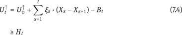
for some predictable process ξ and some increasing process B. Thus, the self-financing trading strategy ![]() = (ξ0, ξ) defined by ξ and the initial capital
= (ξ0, ξ) defined by ξ and the initial capital
is a superhedging strategy for H. Moreover, if ![]() is the value process of any super-hedging strategy, then Lemma 7.8 implies that
is the value process of any super-hedging strategy, then Lemma 7.8 implies that ![]() 0 > E∗[ Hτ ] for all τ ∈ T and each P∗ ∈ P. In particular,
0 > E∗[ Hτ ] for all τ ∈ T and each P∗ ∈ P. In particular, ![]() 0 is larger than any arbitrage-free price for H, and it follows that
0 is larger than any arbitrage-free price for H, and it follows that ![]() 0 ≥ πsup(H). Thus, we have proved:
0 ≥ πsup(H). Thus, we have proved:
Corollary 7.9. There exists a superhedging strategy with initial investment πsup(H), and this is the minimal amount needed to implement a superhedging strategy.
We will call πsup(H) the cost of superhedging of H. Sometimes, a superhedging strategy is also called a superreplication strategy, and one says that πsup(H) is the cost of superreplication or the upper hedging price of H. Recall, however, that πsup(H) is typically not an arbitrage-free price for H. In particular, the seller cannot expect to receive the amount πsup(H) for selling H.
On the other hand, the process B in the decomposition (7.4) can be interpreted as a refunding scheme: Using the superhedging strategy ![]() , the seller may withdraw successively the amounts defined by the increments of B. With this capital flow, the hedging portfolio at time t has the value U↑t ≥ H t. Thus, the seller is on the safe side at no matter when the buyer decides to exercise the option. As we are going to show in Theorem 7.13 below, this procedure is optimal in the sense that, if started at any time t, it requires a minimal amount of capital.
, the seller may withdraw successively the amounts defined by the increments of B. With this capital flow, the hedging portfolio at time t has the value U↑t ≥ H t. Thus, the seller is on the safe side at no matter when the buyer decides to exercise the option. As we are going to show in Theorem 7.13 below, this procedure is optimal in the sense that, if started at any time t, it requires a minimal amount of capital.
Remark 7.10. Suppose πsup(H) belongs to the set Π(H) of arbitrage-free prices for H. By Theorem 6.31, this holds if and only if πsup(H) is the only element of Π(H). In this case, the definition of Π(H) yields a stopping time τ ∈ T and some P∗ ∈ P such that
Now let V be the value process of a superhedging strategy bought at V0 = πsup(H). It follows that E∗[ Vτ ] = πsup(H). Hence, Vτ = Hτ P-a.s., so that H is attainable in the sense of Definition 6.33. This observation completes the proof of Theorem 6.34.
◊
Remark 7.11. If the American claim H is not attainable, then πsup(H) is not an arbitrage-free price of H. Thus, one may expect the existence of arbitrage opportunities if H is traded at the price πsup(H). Indeed, selling H for πsup(H) and buying a superhedging strategy ![]() creates such an arbitrage opportunity: The balance at t = 0 is zero, but Lemma 7.8 implies that the value process V of
creates such an arbitrage opportunity: The balance at t = 0 is zero, but Lemma 7.8 implies that the value process V of ![]() cannot be reached by any exercise strategy σ, i.e., we always have
cannot be reached by any exercise strategy σ, i.e., we always have
Note that (7.5) is not limited to exercise strategies which are stopping times but holds for arbitrary FT-measurable random times σ : Ω → {0, . . . , T}. In other words, πsup(H) is too expensive even if the buyer of H has full information about the future price evolution.
◊
Remark 7.12. The argument of Remark 7.11 implies that an American claim H is attainable if and only if there exists an FT-measurable random time σ : Ω → {0, . . . , T} such that Hσ = Vσ, where V the value process of a superhedging strategy. In other words, the notion of attainability of American claims does not need the restriction to stopping times.
◊
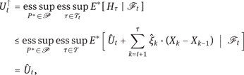
We already know that πsup(H) is the smallest amount for which one can buy a super-hedging strategy at time 0. The following “superhedging duality theorem” extends this result to times t > 0. To this end, denote by ![]() the set of all Ft-measurable random variables
the set of all Ft-measurable random variables ![]() t ≥ 0 for which there exists a d-dimensional predictable process
t ≥ 0 for which there exists a d-dimensional predictable process ![]() such that
such that
Theorem 7.13. The upper Snell envelope ![]() of H is the minimal element of
of H is the minimal element of![]() More precisely:
More precisely:
Proof. Assertion (a) follows immediately from the uniform Doob decomposition of the P-supermartingale U↑. As to part (b), we clearly get ![]() ≥ ess inf
≥ ess inf ![]() from(a).
from(a).
For the proof of the converse inequality, take ![]() and choose a predictable process
and choose a predictable process ![]() for which (7.6) holds. We must show that the set
for which (7.6) holds. We must show that the set ![]() satisfies P[ B ] = 1. Let
satisfies P[ B ] = 1. Let
Then Ût ≤ Ut ↑, and our claim will follow if we can show that U↑t ≤ Ût. Let ξ denote the predictable process obtained from the uniform Doob decomposition of the P-supermartingale U↑, and define

With this choice, Ût satisfies (7.6), i.e.,Ût ∈ U t ↑ (H). Let
Then![]() for all s ≤ t. In particular ÛVt ≥ Ût, and hence ÛVT ≥ H T,which implies that is a P-martingale; see Theorem 5.25. Hence, Doob’s stopping theorem implies
for all s ≤ t. In particular ÛVt ≥ Ût, and hence ÛVT ≥ H T,which implies that is a P-martingale; see Theorem 5.25. Hence, Doob’s stopping theorem implies
which concludes the proof.
We now take the point of view of the buyer of the American claim H. The buyer allocates an initial investment π to purchase H, and then receives the amount H τ ≥ 0. The objective is to find an exercise strategy and a self-financing trading strategy η with initial investment −π, such that the portfolio value is covered by the payoff of the claim. In other words, find τ ∈ T and a self-financing trading strategy with value process V such that V0 = −π and Vτ+Hτ ≥ 0. As shown below, the maximal π for which this is possible is equal to

is the lower Snell envelope of H with respect to the stable set P. More generally, we will consider the buyer’s problem for arbitrary t ≥ 0. To this end, denote by U t ↓ (H) the set of all Ft-measurable random variables ![]() t ≥ 0 for which there exists a d-dimensional predictable process
t ≥ 0 for which there exists a d-dimensional predictable process ![]() and a stopping time σ ∈ Tt such that
and a stopping time σ ∈ Tt such that
Theorem 7.14. ![]() is the maximal element of
is the maximal element of ![]() More precisely:
More precisely:
Proof. (a): Let ![]() be a superhedging strategy for H with initial investment πsup(H), and denote by V the value process of
be a superhedging strategy for H with initial investment πsup(H), and denote by V the value process of ![]() . The main idea of the proof is to use that Vt − H t ≥ 0 can be regarded as a new discounted American claim, to which we can apply Theorem 7.13. However, we must take care of the basic asymmetry of the hedging problem for American options: The seller of H must hedge against all possible exercise strategies, while the buyer must find only one suitable stopping time. It will turn out that a suitable stopping time is given by
. The main idea of the proof is to use that Vt − H t ≥ 0 can be regarded as a new discounted American claim, to which we can apply Theorem 7.13. However, we must take care of the basic asymmetry of the hedging problem for American options: The seller of H must hedge against all possible exercise strategies, while the buyer must find only one suitable stopping time. It will turn out that a suitable stopping time is given by ![]() With this choice, let us define a modified discounted American claim
With this choice, let us define a modified discounted American claim ![]() by
by
Clearly ![]() σ ≤
σ ≤ ![]() τt for all σ ∈ Tt. It follows that
τt for all σ ∈ Tt. It follows that

where we have used that V is a P-martingale in the second and ![]() Theorem 6.47 in the third step. Thus,
Theorem 6.47 in the third step. Thus, ![]() is equal to the upper Snell envelope at time t.
is equal to the upper Snell envelope at time t.
Let ξ be the d-dimensional predictable process obtained from the uniform Doob decomposition of ![]() ↑. Then, due to part (a) of Theorem 7.13,
↑. Then, due to part (a) of Theorem 7.13,
Thus, η := ![]() − ξ is as desired.
− ξ is as desired.
(b): Part (a) implies the inequality ≤ in (b). To prove its converse, take ![]() a d-dimensional predictable process
a d-dimensional predictable process ![]() , and σ ∈ Tt such that
, and σ ∈ Tt such that
We will show below that
Given this fact, we obtain that
for all P∗ ∈ P. Taking the essential infimum over P∗ ∈ P thus yields ![]() t ≤ U↓t and in turn (b).
t ≤ U↓t and in turn (b).
To prove (7.7), let
Then GT ≥ ![]() t− Hσ ≥ −Hσ ∈ L1(P∗) for all P∗, and Theorem 5.14 implies that
t− Hσ ≥ −Hσ ∈ L1(P∗) for all P∗, and Theorem 5.14 implies that ![]() is a P-martingale. Hence (7.7) follows.
is a P-martingale. Hence (7.7) follows.
We conclude this section by stating explicitly the corresponding results for European claims. Recall from Remark 6.6 that every discounted European claim H E can be regarded as the discounted American claim. Therefore, the results we have obtained so far include the corresponding “European” counterparts as special cases.
Corollary 7.15. For any discounted European claim H E such that
there exist two d-dimensional predictable processes ξ and η such that P-a.s.

Remark 7.16. For t = 0, (7.8) takes the form
Thus, the self-financing trading strategy ![]() arising from ξ and the initial investment
arising from ξ and the initial investment ![]() 1 · X0 = supP∗∈P E∗[ HE ] allows the seller to cover all possible obligations without any downside risk. Similarly, (7.9) yields an interpretation of the self-financing trading strategy η which arises from η and the initial investment η1 · X0 = − infP∗∈P E∗[ HE ]. The latter quantity corresponds to the largest loan the buyer can take out and still be sure that, by using the trading strategy η, this debt will be covered by the payoff HE.
1 · X0 = supP∗∈P E∗[ HE ] allows the seller to cover all possible obligations without any downside risk. Similarly, (7.9) yields an interpretation of the self-financing trading strategy η which arises from η and the initial investment η1 · X0 = − infP∗∈P E∗[ HE ]. The latter quantity corresponds to the largest loan the buyer can take out and still be sure that, by using the trading strategy η, this debt will be covered by the payoff HE.
◊
Remark 7.17. Let HE be a discounted European claim such that
Suppose that ![]() ∈ P is such that
∈ P is such that ![]() [ HE ] = πsup(HE). If
[ HE ] = πsup(HE). If ![]() = (ξ0, ξ) is a superhedging strategy for HE, then
= (ξ0, ξ) is a superhedging strategy for HE, then
satisfies HE ≥ HE ≥ 0. Hence, H ÛE is an attainable discounted claim, and it follows from Theorem 5.25 that
This shows that H ÛE and HE are P-a.s. identical and that HE is attainable. We have thus obtained another proof of Theorem 5.32.
◊
As the last result in this section, we formulate the following “superhedging duality theorem”, which states that the bounds in (7.8) and (7.9) are optimal.
Corollary 7.18. Suppose that H E is a discounted European claim with
Denote by U ↑ (HE) the set of all Ft measurable random variables ![]() t for which there t exists a d-dimensional predictable process
t for which there t exists a d-dimensional predictable process ![]() such that
such that
Then
By U t ↓ (HE) we denote the set of all Ft measurable random variables ![]() t for which there exists a d-dimensional predictable process
t for which there exists a d-dimensional predictable process ![]() such that
such that
Then
Remark 7.19. Define A as the set of financial positions Z ∈ L∞(Ω,FT , P) which are acceptable in the sense that there exists a d-dimensional predictable process ξ such that
As in Section 4.8, this set A induces a coherent risk measure ρ on L∞(Ω,FT , P):
Corollary 7.18 implies that ρ can be represented as
We therefore obtain a multiperiod version of Proposition 4.99.
◊
Remark 7.20. Often, the superhedging strategy in a given incomplete model can be identified as the perfect hedge in an associated “extremal” model. As an example, consider a one-period model with d discounted risky assets given by bounded random variables X1, . . . , Xd. Denote by μ the distribution of X = (X1, . . . , Xd) and by Γ(μ) the convex hull of the support of μ. The closure K := Γ(μ) of Γ(μ) is convex and compact. We know from Section 1.5 that the model is arbitrage-free if and only if the price system π = (π1, . . . , πd) is contained in the relative interior of Γ(μ), and the equivalent martingale measures can be identified with the measures μ∗ ≈ μ with barycenter π. Consider a derivative H = h(X) given by a convex function h on K. The cost of superhedging is given by
which is a special case of the duality result of Theorem 1.32. Since {α ≥ h} is convex and closed, the condition μ(α ≥ h) = 1 implies α ≥ h on K. Denote by M(π) the class of all probability measures on K with barycenter π. For any affine function α with α ≥ h on K, and for any ![]() ∈ M(π) we have
∈ M(π) we have
Thus,
where we define for f ∈ C(K)
The supremum in (7.10) is attained since M(π) is weakly compact. More precisely, it is attained by any measure Ûμ ∈ M(π) on K which is maximal with respect to the balayage order ≽bal defined for measures on K as in (2.25); see Théorème X. 41 in [90]. But such a maximal measure is supported by the set of extreme points of the convex compact set K, i.e., by the Choquet boundary of K. This follows from a general integral representation theorem of Choquet; see, e.g., Théorème X. 43 of [90]. In our finite-dimensional setting, Ûμ can in fact be chosen to have a support consisting of at most d + 1 points, due to a theorem of Carathéodory and the representation of K as the convex hull of its extreme points; see [232], Theorems 17.1 and 18.5. But this means that Ûμ can be identified with a complete model, due to Proposition 1.41. Thus, the cost of superhedging Ûh(π) can be identified with the canonical price
of the derivative H, computed in the complete model Ûμ. Note that Ûμ sits on the Choquet boundary of K = Γ(μ), but typically it will no longer be equivalent or absolutely continuous with respect to the original measure μ. As a simple illustration, consider a one-period model with one risky asset X1. If X1 is bounded, then the distribution μ of X1 has bounded support, and Γ(μ) is of the form [a, b]. In this case, the cost of superhedging H = h(X1) for a convex function h is given by the price
computed in the binary model in which X1 takes only the values a and b, and where p∗ ∈ (0, 1) is determined by
◊
The following example illustrates that a superhedging strategy is typically too expensive from a practical point of view. However, we will see in Chapter 8 how superhedging strategies can be used in order to construct other hedging strategies which are efficient in terms of cost and shortfall risk.
Example 7.21. Consider a simple one-period model where Shas under P 1a 1Poisson distribution and where S0 ≡ 1. Let ![]() be a call option with strike > 0. We have seen in Example 1.38 that πinf(H) and πsup(H) coincide with the universal arbitrage bounds of Remark 1.37:
be a call option with strike > 0. We have seen in Example 1.38 that πinf(H) and πsup(H) coincide with the universal arbitrage bounds of Remark 1.37:
Thus, the superhedging strategy for the seller consists in the trivial hedge of buying the asset at time 0, while the corresponding strategy for the buyer is a short-sale of the asset in case the option is in the money, i.e., if ![]()
◊
7.4Superhedging with liquid options
In practice, some derivatives such as put or call options are traded so frequently that their prices are quoted just like those of the primary assets. The prices of such liquid options can be regarded as an additional source of information on the expectations of the market as to the future evolution of asset prices. This information can be exploited in various ways. First, it serves to single out those martingale measures P∗ which are compatible with the observed options prices, in the sense that the observed prices coincide with the expectations of the discounted payoff under P∗. Second, liquid options may be used as instruments for hedging more exotic options.
Our aim in this section is to illustrate these ideas in a simple setting. Assume that there is only one risky asset S1 such that ![]() is a positive constant, and that S0 is a riskless bond with interest rate r = 0. Thus, the discounted price process of the risky asset is given by
is a positive constant, and that S0 is a riskless bond with interest rate r = 0. Thus, the discounted price process of the risky asset is given by ![]() for t = 0, . . . , T. As the underlying space of scenarios, we use the product space
for t = 0, . . . , T. As the underlying space of scenarios, we use the product space
We define Xt(ω) = xt for ω = (x1, . . . , xT) ∈ Ω, and denote by Ft the σ-algebra generated by X0, . . . , Xt; note that F0 = {∅, Ω}. No probability measure P is given a priori. Let us now introduce a linear space X of FT-measurable functions as the smallest linear space such that the following conditions are satisfied:
(a) 1 ∈ X .
(b) (Xt − Xs) ![]() A ∈ X for 0 ≤ s < t ≤ T and A ∈ Fs.
A ∈ X for 0 ≤ s < t ≤ T and A ∈ Fs.
(c) (Xt − K)+ ∈ X for K ≥ 0 and t = 1, . . . , T.
The functions in the space X will be interpreted as (discounted) payoffs of liquid derivatives. The constant 1 in (a) corresponds to a unit investment into the riskless bond. The function Xt − Xs in (b) corresponds to the payoff of a forward contract on the risky asset, issued at time s for the price Xs and expiring at time t. The decision to buy such a forward contract at time s may depend on the market situation at time s; this is taken into account by allowing for payoffs (Xt − Xs) ![]() A with A ∈ Fs. Linearity of X together with conditions (a) and (b) implies that
A with A ∈ Fs. Linearity of X together with conditions (a) and (b) implies that
Finally, condition (c) states that call options with any possible strike and any maturity up to time T can be used as liquid securities.
Suppose that a linear pricing rule Φ is given on X . The value Φ(Y) will be interpreted as the market price of the liquid security Y ∈ X . The price of a liquid call option with strike K and maturity t will be denoted by
Assumption 7.22. We assume thatΦ : X → ℝ is a linear functional which satisfies the following conditions.
(a) Φ(1) = 1.
(b) Φ(Y) ≥ 0 if Y ≥ 0.
(c) Φ(Xt − Xs) ![]() A = 0 for all 0 ≤ s < t ≤ T and A ∈ Fs.
A = 0 for all 0 ≤ s < t ≤ T and A ∈ Fs.
(d) Ct(K) = Φ(Xt − K)+→ 0 as K ↑ ∞for all t.
The first two conditions must clearly be satisfied if the pricing rule Φ shall not create arbitrage opportunities. Condition (c) states that Xs is the fair price for a forward contract issued at time s. This condition is quite natural in view of Theorem 5.29. In our present setting, it can also be justified by the following simple replication argument. At time s, take out a loan Xs(ω) and use it for buying the asset. At time t, the asset is worth X t(ω) and the loan must be paid back, which results in a balance Xt(ω) − Xs(ω). Since this investment strategy requires zero initial capital, the price of the corresponding payoff should also be zero. The continuity condition (d) is also quite natural.
Our first goal is to show that any such pricing rule Φ is compatible with the paradigm that arbitrage-free prices can be identified as expectations with respect to some martingale measure for X. More precisely, we are going to construct a martingale measure P∗ such that Φ(Y) = E∗[ Y ] for all Y ∈ X . On the one hand, this will imply regularity properties of Φ. On the other hand, this will yield an extension of our pricing rule Φ to a larger space of payoffs including path-dependent exotic options. As a first step in this direction, we have the following result.
Lemma 7.23. For each t, there exists a unique probability measure μt on [0,∞) such that for all K ≥ 0
In particular, μt has the mean
Proof. Since ![]() is convex and decreasing, linearity and positivity of Φ imply that the function ϕt(K) := Φ(Xt −K)+is convex and decreasing as well. Hence, C t(K) admits a right-hand derivative, denoted by −f (K) in the sequel. The function f is then right-continuous, decreasing, and such that
is convex and decreasing, linearity and positivity of Φ imply that the function ϕt(K) := Φ(Xt −K)+is convex and decreasing as well. Hence, C t(K) admits a right-hand derivative, denoted by −f (K) in the sequel. The function f is then right-continuous, decreasing, and such that
Our fourth condition on Φ yields
so that f (x) ↘ 0 as x ↑ ∞. Hence, there exists a positive measure μt on (0,∞) such that
Fubini’s theorem implies
and

It remains to show that μt can be extended to a probability measure on [0, ∞), i.e., we must show that μt(0,∞)≤ 1. To this end, we will use the “put-call parity”
which follows from our assumptions on Φ. Thus,
where g(x) = 1 − f (x). Since ![]() is increasing, g must be nonnegative, and we obtain 1 ≥ f (0) = μt(0,∞).
is increasing, g must be nonnegative, and we obtain 1 ≥ f (0) = μt(0,∞).
The following lemma shows that the measures μt constructed in Lemma 7.23 are related to each other by the balayage order ≽bal, defined by
for probability measures with finite expectation; see Remark 2.63 and recall that ≽bal is also called the convex stochastic order.
Lemma 7.24. The map t μt is increasing with respect to the balayage order ≽bal:

Since the price of the forward contract ![]() vanishes under our pricing rule Φ, we must have that for all K ≥ 0
vanishes under our pricing rule Φ, we must have that for all K ≥ 0
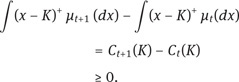
An application of Corollary 2.61 concludes the proof.
Let us introduce the class
of all probability measures P∗ on (Ω,F) which coincide with Φ on X . Note that for any P∗ ∈ PΦ,
so that PΦ consists of martingale measures for X. Our first main result in this section can be regarded as a version of the “fundamental theorem of asset pricing” without an a priori measure P.
Theorem 7.25. Under Assumption 7.22, the class PΦ is nonempty. Moreover, there exists P∗ ∈ PΦ with the Markov property: For 0 ≤ s ≤ t ≤ T and each bounded measurable function f ,
Proof. Since μt+1 ≽bal μt, Corollary 2.61 yields the existence of a stochastic kernel Qt+1 ∫ such that y Qt+1(x, dy) = x and μt+1 = μtQt+1. Let us define
i.e., for each measurable set A ⊂ Ω = [0,∞)T
Clearly, μt is the law of X t under P∗. In particular, all call options are priced correctly by calculating their expectation with respect to P∗. Then one checks that P∗-a.s.
The first identity above implies E∗[ Xt+1 | Ft ] = Xt. In particular, P∗ is a martingale measure, and the expectation of (Xt − Xs) ![]() A vanishes for s < t and A ∈ Fs. It follows that E∗[ Y ] = Φ(Y) for all Y ∈ X . Finally, an induction argument applied to (7.11) yields the Markov property.
A vanishes for s < t and A ∈ Fs. It follows that E∗[ Y ] = Φ(Y) for all Y ∈ X . Finally, an induction argument applied to (7.11) yields the Markov property.
So far, we have assumed that our space X of liquidly traded derivatives contains call options with all possible strike prices and maturities. From now on, we will simplify our setting by assuming that only call options with maturity T are liquidly traded. Thus, we replace X by the smaller space XT which is defined as the linear hull of the constants, of all forward contracts
and of all call options
with maturity T. The observed market prices of derivatives in XT are as before modeled by a linear pricing rule
We assume that ΦT satisfies Assumption 7.22 in the sense that condition (d) is only required for t = T:
(dʹ) CT(K) := ΦT(XT − K)+→ 0 as K ↑ ∞.
By
we denote the class of all probability measures P∗ on (Ω,F) which coincide with ΦT on XT. As before, it follows from condition (c) of Assumption 7.22 that any P∗ ∈ PΦTwill be a martingale measure for the price process X. Obviously, any linear pricing rule Φ which is defined on the full space X and which satisfies Assumption 7.22 can be restricted to XT, and this restriction satisfies the above assumptions. Thus, we have ![]()
Proposition 7.26. Under the above assumptions,![]() is nonempty.
is nonempty.
Proof. Let μT be the measure constructed in Lemma 7.23 from the call prices with maturity T. Now consider the measure ![]() on (Ω,F) defined as
on (Ω,F) defined as
i.e., under ![]() we have Xt = X0
we have Xt = X0![]() -a.s. for t < T, and the law of X T is μT. Clearly, we have
-a.s. for t < T, and the law of X T is μT. Clearly, we have ![]()
A measure ![]() can be regarded as an extension of the pricing rule ΦT to the larger space L1(P∗), and the expectation E∗[ H ] of some European claim H ≥ 0 can be regarded as an arbitrage-free price for H. Our aim is to obtain upper and lower bounds for E∗[ H ]which hold simultaneously for all P∗ ∈ PΦ.We will derive such bounds for various exotic options; this will amount to the construction of certain superhedging strategies in terms of liquid securities.
can be regarded as an extension of the pricing rule ΦT to the larger space L1(P∗), and the expectation E∗[ H ] of some European claim H ≥ 0 can be regarded as an arbitrage-free price for H. Our aim is to obtain upper and lower bounds for E∗[ H ]which hold simultaneously for all P∗ ∈ PΦ.We will derive such bounds for various exotic options; this will amount to the construction of certain superhedging strategies in terms of liquid securities.
As a first example, we consider the following digital option

which has a unit payoff if the price process reaches a given upper barrier B > X0. If we denote by
the first hitting time of the barrier B, then the payoff of the digital option can also be described as
For simplicity, we will assume from now on that
so that in particular μT(B,∞) > 0.
Theorem 7.27. The following upper bound on the arbitrage-free prices of the digital option holds:
Proof. For 0 ≤ K < B, we have XτB ≥ B. Hence,
Taking expectations with respect to some P∗ ∈ PΦT yields
Since P∗ is a martingale measure, the stopping theorem in the form of Proposition 6.37 implies
This shows that
The proof will be completed by Lemmas 7.28 and 7.29 below.
Lemma 7.28. If we let
then the infimum on the right-hand side is attained in K if and only if K belongs to the set of λ-quantiles for μT, i.e., if and only if
In particular, it is attained in
Proof. The convex function C T has left- and right-hand derivatives
see also Proposition A.7. Thus, the function g(K) := CT(K)/(B − K) has a minimum in K if and only if its left- and right-hand derivatives satisfy
By computing ![]() and
and ![]() one sees that these two conditions are equivalent to the requirement that K is a λ-quantile for μT; see Lemma A.19.
one sees that these two conditions are equivalent to the requirement that K is a λ-quantile for μT; see Lemma A.19. ![]()
Lemma 7.29. There exists a martingale measure![]() such that
such that
Moreover, ![]() can be taken such that
can be taken such that
and
where K∗ is as in Lemma 7.28.
Proof. Let λ be as in Lemma 7.28, and let
be the lower quantile function for μ; see A.3. We take an auxiliary probability space (![]() , F,
, F,![]() ) supporting a random variable U which is uniformly distributed on (0, 1). By Lemma A.23,
) supporting a random variable U which is uniformly distributed on (0, 1). By Lemma A.23,![]() T := q(U) has distribution μT under
T := q(U) has distribution μT under ![]() . Let γ be such that
. Let γ be such that
Since B > X0 we have 0 ≤ γ < X0. We define ![]() T−1 by
T−1 by
and we let ![]() t := X0 for 0 ≤ t ≤ T − 2.
t := X0 for 0 ≤ t ≤ T − 2.
We now prove that ![]() is a martingale with respect to its natural filtration Ft := σ(
is a martingale with respect to its natural filtration Ft := σ(![]() 0, . . . ,
0, . . . ,![]() t). To this end, note first that FT−2 = {∅,
t). To this end, note first that FT−2 = {∅,![]() }, and hence
}, and hence
Furthermore, since K ∗ = q(λ),

Hence,

It follows that
and so ![]() is indeed a martingale.
is indeed a martingale.
As the next step, we note that

where we have used the fact that K ∗ = q(λ). Hence, if we denote by
the first time at which ![]() hits the barrier B, then
hits the barrier B, then
Hence, {![]() B ≤ T} = {
B ≤ T} = {![]() B = T − 1} = {
B = T − 1} = {![]() T−1 = B},
T−1 = B},
and the distribution ![]() of
of ![]() under
under ![]() is as desired.
is as desired.
Remark 7.30. The inequality
appearing in the proof of Theorem 7.27 can be interpreted in terms of a suitable superhedging strategy for the claim Hdig by using call options and forward contracts: At time t = 0, we buy (B − K)−1 call options with strike K, and at the first time when the price process passes the barrier B, we sell forward (B − K)−1 shares of the asset. This strategy will be optimal if the strike price K is such that it realizes the minimum on the right-hand side of (7.12). By virtue of Lemma 7.28, such an optimal strike price can be identified as the Value at Risk at level 1 − λ of a short position −XT in the asset.
◊
Let us now derive bounds on the arbitrage-free prices of barrier call options. More precisely, we will consider an up-and-in call option

and the corresponding up-and-out call

If the barrier B is below the strike price K, then the up-and-in call is identical to a “plain vanilla call” (XT − K)+, and the payoff of the up-and-out call is zero. Thus, we assume from now on that
K < B.
Recall that K ∗ denotes the minimizer of the function c CT(c)/(B − c) as constructed in Lemma 7.28.
Theorem 7.31. For an up-and-in call option,

Proof. For any c with K ≤ c < B,
Indeed, on {XT ≤ K } or on {τB > T} the payoff of ![]() is zero, and the right-hand side is nonnegative. On {XT ≥ c, τB ≤ T} and on {c > XT > K, τB ≤ T} we have ≤. The expectation of the right-hand side under a martingale measure P∗ ∈ PΦT is equal to
is zero, and the right-hand side is nonnegative. On {XT ≥ c, τB ≤ T} and on {c > XT > K, τB ≤ T} we have ≤. The expectation of the right-hand side under a martingale measure P∗ ∈ PΦT is equal to
due to the stopping theorem. The minimum of this upper bound over all c ∈ [K, B) is attained in c = K ∨ K ∗, which shows ≤ in the assertion.
Finally, let ![]() be the martingale measure constructed in Lemma 7.29. If K ∗ ≤ K then
be the martingale measure constructed in Lemma 7.29. If K ∗ ≤ K then
and so![]() If K∗ > K then
If K∗ > K then ![]() -a.s.
-a.s.
Taking expectations with respect to ![]() concludes the proof.
concludes the proof.
Remark 7.32. The inequality
appearing in the preceding proof can be interpreted as a superhedging strategy for the up-and-in call with liquid derivatives: At time t = 0, we purchase (B − K)/(B − c) call options with strike c, and at the first time when the stock price passes the barrier B, we sell forward (c − K)/(B − c) shares of the asset. This strategy will be optimal for c = K ∗ ∨ K.
◊
We now turn to the analysis of the up-and-out call option
Theorem 7.33. For an up-and-out call,
Proof. Clearly,

Taking expectations yields ≤ in the assertion.
Now consider the measure ![]() on (Ω,F) defined as
on (Ω,F) defined as
i.e., under ![]() we have Xt = X0
we have Xt = X0 ![]() -a.s. for t < T, and the law of XT is μT. Clearly
-a.s. for t < T, and the law of XT is μT. Clearly![]() and (7.13) is
and (7.13) is ![]() -a.s. an identity.
-a.s. an identity.
Using the identity
we get the following lower bounds as an immediate corollary.
Corollary 7.34. We have
and
