
Chapter 10. Strain Gauges, Load Cells, and Weighing
10.1. Introduction
Accurate measurement of weight is required in many industrial processes. There are two basic techniques in use. In the first, shown in Figure 10.1(A) and called a force balance system, the weight of the object is opposed by some known force which will equal the weight. Kitchen scales where weights are added to one pan to balance the object in the other pan use the force balance system. Industrial systems use hydraulic or pneumatic pressure to balance the load, the pressure required being directly proportional to the weight.
Figure 10.1. The two different weighing principles: (A) force balance; (B) strain.

The second, and commoner, method is called strain weighing and uses the gravitational force from the load to cause a change in the structure which can be measured. The simplest form is the spring balance of Figure 12.1(B) where the deflection is proportional to the load.
10.2. Stress and Strain
The application of a force to an object will result in deformation of the object. In Figure 10.2 a tensile force F has been applied to a rod of cross-sectional area A and length L. This results in an increase in length ΔL. The effect of the force will depend on the force and the area over which it is applied. This is called the stress and is the force per unit area:
![]()
Figure 10.2. Tensile strain.

Stress has the units of N/m2 (i.e., the same as pressure, so pascals are sometimes used).
The resulting deformation is called the strain and is defined as the fractional change in length.
![]()
Strain is dimensionless. Because the change in length is small, microstrain (μstrain defined as strain × 106) is often used. A 10-m rod exhibiting a change in length of 0.0045 mm because of an applied force is exhibiting 45 μstrain.
The strain will increase as the stress increases as shown in Figure 10.3. Over region AB the object behaves as a spring; the relationship is linear and there is no hysteresis (i.e., the object returns to its original dimension when the force is removed). Beyond Point B the object suffers deformation and the change is not reversible. The relationship is now nonlinear, and with increasing stress the object fractures at point C. The region AB, called the elastic region, is used for strain measurement. Point B is called the elastic limit. Typically AB will cover a range of 10,000 μstrain.
Figure 10.3. The relationship between stress and strain.

The inverse slope of the line AB is sometimes called the elastic modulus (or modulus of elasticity). It is more commonly known as Young's modulus defined as
![]()
Young's modulus has dimensions of Nm−2, that is, the same as pressure. It is commonly given in pascals. Typical values are:
- Steel 210 GPa
- Copper 120 GPa
- Aluminium 70 GPa
- Plastics 30 GPa
When an object experiences strain, it displays not only a change in length but also a change in cross-sectional area. This is defined by Poisson's ratio, denoted by the Greek letter ν. If an object has a length L and width W in its unstrained state and experiences changes ΔL and ΔW when strained, Poisson's ratio is defined as
![]()
Typically ν is between 0.2 and 0.4. Poisson's ratio can be used to calculate the change in cross-sectional area.
10.3. Strain Gauges
The electrical resistance of a conductor is proportional to the length and inversely proportional to the cross-section; that is,
![]() where ρ is a constant called the resistivity of the material.
where ρ is a constant called the resistivity of the material.
When a conductor suffers stress, its length and area will both change resulting in a change in resistance. For tensile stress, the length will increase and the cross-sectional area decrease both resulting in increased resistance. Similarly the resistance will decrease for compressive stress.
Ignoring second-order effects the change in resistance is given by (10.1)
![]() where G is a constant called the gauge factor. ΔL/L is the strain, E, so Equation (10.1) can be rewritten (10.2)
where G is a constant called the gauge factor. ΔL/L is the strain, E, so Equation (10.1) can be rewritten (10.2)
![]() where E is the strain experienced by the conductor.
where E is the strain experienced by the conductor.
Devices based on the change of resistance with load are called strain gauges, and Equation (10.2) is the fundamental strain gauge equation.
Practical strain gauges are not a slab of material as implied so far but consist of a thin, small (typically a few millimeters) foil similar to Figure 10.4 with a pattern to increase the conductor length and hence the gauge factor. The gauge is attached to some sturdy stressed member with epoxy resin and experiences the same strain as the member. Early gauges were constructed from thin wire but modern gauges are photoetched from metallized film deposited onto a polyester or plastic backing. Normal gauges can experience up to 10,000 μstrain without damage. Typically the design will aim for 2000 μstrain under maximum load.
Figure 10.4. A typical strain gauge

(courtesy of Welwyn Strain Measurements).
A typical strain gauge will have a gauge factor of 2, a resistance of 120Ω, and experience 1000 μstrain. From Equation (10.2) this will result in a resistance change of 0.24Ω.
Strain gauges must ignore strains in unwanted directions. A gauge has two axes, an active axis along which the strain is applied and a passive axis (usually at 90°) along which the gauge is least sensitive. The relationship between these is defined by the cross-sensitivity:
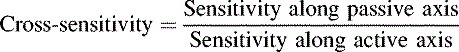
Cross-sensitivity is typically about 0.002.
10.4. Bridge Circuits
The small change in resistance is superimposed on the large unstrained resistance. Typically the change will be 1 part in 5000. In Figure 10.5 the strain gauge Rg is connected into a classical Wheatstone bridge. In the normal laboratory method, Ra and Rb are made equal and calibrated resistance box Rc adjusted until V0 (measured by a sensitive millivoltmeter) is zero. Resistance Rc then equals Rg.
Figure 10.5. Simple measurement of strain with a Wheatstone bridge.
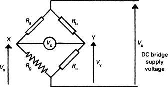
With a strain gauge however, we are not interested in the actual resistance, but the change caused by the applied load. Suppose Rb and Rc are made equal, and Ra is made equal to the unloaded resistance of the strain gauge. Voltages V1 and V2 will both be half the supply voltage and V0 will be zero. If a load is applied to the strain gauge such that its resistance changes by fractional change x (i.e., x = ΔR/R) it can be shown that (10.3)
![]()
In a normal circuit x will be very small compared with 2. For the earlier example x has the value 0.24/120 = 0.002, so Equation (10.3) can be simplified to
![]()
But ΔR = E · G · R where E is the strain and G the gauge factor, giving (10.4)
![]()
For small values of x, the output voltage is thus linearly related to the strain.
It is instructive to put typical values into Equation (10.4). For a 24-V supply, 1000 μstrain, and gauge factor 2, we get 12 mV. This output voltage must be amplified before it can be used. Care must be taken to avoid common mode noise, so the differential amplifier circuit of Figure 10.6 is commonly used.
Figure 10.6. Differential amplifier. The output voltage is determined by the difference between the two input voltages.
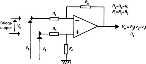
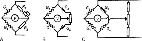
Resistance changes from temperature variation are of a similar magnitude to resistance changes from strain. The simplest way of preventing this is to use two gauges arranged as Figure 10.7(A). One gauge has its active axis and the other gauge the passive axis aligned with the load. If these are connected into a bridge circuit as shown on Figure 10.7(B) both gauges will exhibit the same resistance change from temperature and these will cancel leaving the output voltage purely dependent on the strain.
Figure 10.7. Use of multiple strain gauges: (A) two gauges used to give temperature compensation; (B) two gauges connected into bridge—temperature effects will affect both gauges equally and have no effect; (C) four-gauge bridge gives increased sensitivity and temperature compensation; (D) arrangement for four gauges—two will be in compression and two in tension for load changes. Temperature affects all gauges equally.
Temperature errors can also occur from dimensional changes in the member to which the strain gauges are attached. Gauges are often temperature compensated by having coefficients of linear expansion identical to the material to which they are attached.
Many applications use gauges in all four arms of the bridge as shown in Figure 10.7(C) with two active gauges and two passive gauges. This provides temperature compensation and doubles the output voltage, giving
![]()
In the arrangement of Figure 10.7(D) four gauges are used with two gauges experiencing compressive strain and two experiencing tensile strain. Here all four gauges are active, giving (10.5)
![]()
Again temperature compensation occurs because all gauges are at the same temperature.
Gauges are manufactured to a tolerance of about 0.5%, that is, about ±0.6Ω for a typical 120-Ω gauge. As this is larger than the resistance change from strain some form of zeroing will be required. Three methods of achieving this are shown in Figure 10.8. Arrangements b and c are preferred if the zeroing is remote from the bridge.
Figure 10.8
Equation (10.5) shows that the output voltage is directly related to the supply voltage. This implies that a large voltage should be used to increase the sensitivity. Unfortunately a high-voltage supply cannot be used or I2R heating in the gauges will cause errors and ultimately failure. Bridge voltages of 15–30V and currents of 20–100 mA are typically used.
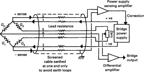
Equation (10.5) also implies that the supply voltage must be stable. If the bridge is remote from the supply and electronics, as is usually the case, voltage drops down the cabling can introduce significant errors. Figure 10.9 shows a typical cabling scheme used to give remote zeroing and compensation for cabling resistance. The supply is provided on cores 2 and 6 and monitored on cores 1 and 7 to keep constant voltage at the bridge itself.
Figure 10.9
10.5. Load Cells
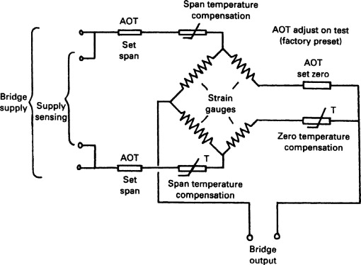
A load cell converts a force (usually the gravitational force from an object being weighed) to a strain which can then be converted to an electrical signal by strain gauges. A load cell will typically have the local circuit of Figure 10.10 with four gauges, two in compression and two in tension, and six external connections. The span and zero adjust on test (AOT) are factory set to ensure the bridge is within limits that can be further adjusted on site. The temperature compensation resistors compensate for changes in Young's modulus with temperature, not changes of the gauges themselves which the bridge inherently ignores.
Figure 10.10
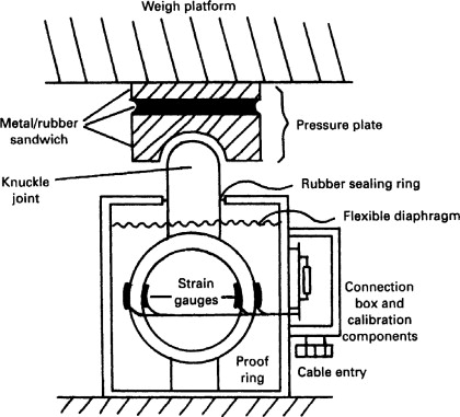
Coupling of the load requires care, a typical arrangement being shown on Figure 10.11. A pressure plate applies the load to the proof-ring via a knuckle and avoids error from slight misalignment. A flexible diaphragm seals against dust and weather. A small gap ensures that shock overloads will make the load cell bottom out without damage to the proof-ring or gauges. Maintenance must ensure that dust does not close this gap and cause the proof-ring to carry only part of the load. Bridging and binding are common causes of load cells reading below the load weight.
Figure 10.11
Multicell weighing systems can be used, with the readings from each cell being summed electronically. Three cell systems inherently spread the load across all cells. With four cell systems the support structure must ensure that all cells are in contact with the load at all times.
Usually the load cells are the only route to ground from the weigh platform. It is advisable to provide a flexible earth strap, not only for electrical safety but also to provide a route for any welding current which might arise from repairs or later modification.
10.6. Weighing Systems
A weigh system is usually more than a collection of load cells and a display. Figure 10.12 is a taring weigh system used when a “recipe” of several materials is to be collected in a hopper. The gross weight is the weight from the load cells, that is, the materials and the hopper itself. Each time the tare command is given, the gross weight is stored and this stored value subtracted from the gross weight to give the net weight display. In this way the weight of each new material can be clearly seen. This type of weigh system can obviously be linked into a supervisory PLC or computer control network.
Figure 10.12
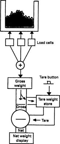
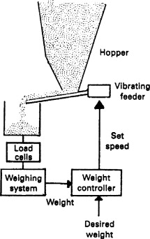
Figure 10.13 is a batch feeder system where material is fed from a vibrating feeder into a weigh hopper. The system is first tared, then a two-speed system used with a changeover from fast to dribble feed a preset weight before the target weight. The feeder turns off just before the correct weight to allow for the material in flight from the feeder. This is known as in-flight compensation, anticipation, or preact. To reduce the weigh time the fast feed should be set as fast as possible without causing avalanching in the feed hopper and the changeover to slow feed made as late as possible. The accuracy of the system is mainly dependent on the repeatability of the preact weight, so the slow speed should be set as low as possible.
Figure 10.13
Material is often carried on conveyor belts and Figure 10.14 shows a method of providing feed rate in weight per unit time (e.g., kilogram per minute).
Figure 10.14
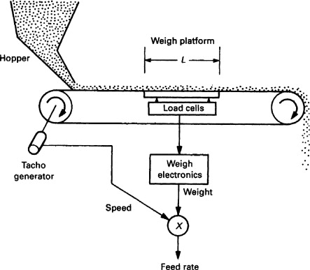
The conveyor passes over a load cell of known length and the linear speed is obtained from the drive motor, probably from a tachogenerator. If the weigh platform has length L m, and is indicating weight W kg at speed V ms−1, the feed rate is simply W · V/L kgs−1.