Chapter 2. Sensors and Transducers

2.1. Basic Sensor Technology

A sensor is a device that converts a physical phenomenon into an electrical signal. As such, sensors represent part of the interface between the physical world and the world of electrical devices, such as computers. The other part of this interface is represented by actuators, which convert electrical signals into physical phenomena.

Why do we care so much about this interface? In recent years, enormous capability for information processing has been developed within the electronics industry. The most significant example of this capability is the personal computer. In addition, the availability of inexpensive microprocessors is having a tremendous impact on the design of embedded computing products ranging from automobiles to microwave ovens to toys. In recent years, versions of these products that use microprocessors for control of functionality are becoming widely available. In automobiles, such capability is necessary to achieve compliance with pollution restrictions. In other cases, such capability simply offers an inexpensive performance advantage.

All of these microprocessors need electrical input voltages in order to receive instructions and information. So, along with the availability of inexpensive microprocessors has grown an opportunity for the use of sensors in a wide variety of products. In addition, since the output of the sensor is an electrical signal, sensors tend to be characterized in the same way as electronic devices. The data sheets for many sensors are formatted just like electronic product data sheets.

However, there are many formats in existence, and there is nothing close to an international standard for sensor specifications. The system designer will encounter a variety of interpretations of sensor performance parameters, and it can be confusing. It is important to realize that this confusion is not due to an inability to explain the meaning of the terms—rather it is a result of the fact that different parts of the sensor community have grown comfortable using these terms differently.

2.1.1. Sensor Data Sheets

It is important to understand the function of the data sheet in order to deal with this variability. The data sheet is primarily a marketing document. It is typically designed to highlight the positive attributes of a particular sensor and emphasize some of the potential uses of the sensor, and it might neglect to comment on some of the negative characteristics of the sensor. In many cases, the sensor has been designed to meet a particular performance specification for a specific customer, and the data sheet will concentrate on the performance parameters of greatest interest to this customer. In this case, the vendor and customer might have grown accustomed to unusual definitions for certain sensor performance parameters. Potential new users of such a sensor must recognize this situation and interpret things reasonably. Odd definitions may be encountered here and there, and most sensor data sheets are missing some pieces of information that are of interest to particular applications.

2.1.2. Sensor Performance Characteristics Definitions

The following are some of the more important sensor characteristics.

2.1.2.1. Transfer Function

The transfer function shows the functional relationship between physical input signal and electrical output signal. Usually, this relationship is represented as a graph showing the relationship between the input and output signal, and the details of this relationship may constitute a complete description of the sensor characteristics. For expensive sensors that are individually calibrated, this might take the form of the certified calibration curve.

2.1.2.2. Sensitivity

The sensitivity is defined in terms of the relationship between input physical signal and output electrical signal. It is generally the ratio between a small change in electrical signal to a small change in physical signal. As such, it may be expressed as the derivative of the transfer function with respect to physical signal. Typical units are volts/kelvins, millivolts/kilopascals, and the like. A thermometer would have “high sensitivity” if a small temperature change resulted in a large voltage change.

2.1.2.3. Span or Dynamic Range

The range of input physical signals that may be converted to electrical signals by the sensor is the dynamic range or span. Signals outside of this range are expected to cause unacceptably large inaccuracy. This span or dynamic range is usually specified by the sensor supplier as the range over which other performance characteristics described in the data sheets are expected to apply. Typical units are kelvins, pascals, and newtons.

2.1.2.4. Accuracy or Uncertainty

Uncertainty is generally defined as the largest expected error between actual and ideal output signals. Typical units are kelvins. Sometimes this is quoted as a fraction of the full-scale output or a fraction of the reading. For example, a thermometer might be guaranteed accurate to within 5% of FSO (full-scale output). Accuracy is generally considered by metrologists to be a qualitative term, while uncertainty is quantitative. For example, one sensor might have better accuracy than another if its uncertainty is 1% compared to the other with an uncertainty of 3%.

2.1.2.5. Hysteresis

Some sensors do not return to the same output value when the input stimulus is cycled up or down. The width of the expected error in terms of the measured quantity is defined as the hysteresis. Typical units are kelvins or percent of FSO.

2.1.2.6. Nonlinearity (Often Called Linearity)

Nonlinearity is the maximum deviation from a linear transfer function over the specified dynamic range. There are several measures of this error. The most common compares the actual transfer function with the “best straight line,” which lies midway between the two parallel lines that encompass the entire transfer function over the specified dynamic range of the device. This choice of comparison method is popular because it makes most sensors look the best. Other reference lines may be used, so the user should be careful to compare using the same reference.

2.1.2.7. Noise

All sensors produce some output noise in addition to the output signal. In some cases, the noise of the sensor is less than the noise of the next element in the electronics or less than the fluctuations in the physical signal, in which case it is not important. Many other cases exist in which the noise of the sensor limits the performance of the system based on the sensor. Noise is generally distributed across the frequency spectrum. Many common noise sources produce a white noise distribution, which is to say that the spectral noise density is the same at all frequencies. Johnson noise in a resistor is a good example of such a noise distribution. For white noise, the spectral noise density is characterized in units of volts/root (Hz). A distribution of this nature adds noise to a measurement with amplitude proportional to the square root of the measurement bandwidth. Since there is an inverse relationship between the bandwidth and measurement time, it can be said that the noise decreases with the square root of the measurement time.

2.1.2.8. Resolution

The resolution of a sensor is defined as the minimum detectable signal fluctuation. Since fluctuations are temporal phenomena, there is some relationship between the timescale for the fluctuation and the minimum detectable amplitude. Therefore, the definition of resolution must include some information about the nature of the measurement being carried out. Many sensors are limited by noise with a white spectral distribution. In these cases, the resolution may be specified in units of physical signal/root (Hz). Then, the actual resolution for a particular measurement may be obtained by multiplying this quantity by the square root of the measurement bandwidth. Sensor data sheets generally quote resolution in units of signal/root (Hz) or they give a minimum detectable signal for a specific measurement. If the shape of the noise distribution is also specified, it is possible to generalize these results to any measurement.

2.1.2.9. Bandwidth

All sensors have finite response times to an instantaneous change in physical signal. In addition, many sensors have decay times, which would represent the time after a step change in physical signal for the sensor output to decay to its original value. The reciprocal of these times corresponds to the upper and lower cutoff frequencies, respectively. The bandwidth of a sensor is the frequency range between these two frequencies.

2.1.3. Sensor Performance Characteristics of an Example Device

To add substance to these definitions, we identify the numerical values of these parameters for an off-the-shelf accelerometer, Analog Devices's ADXL150.

2.1.3.1. Transfer Function

The functional relationship between voltage and acceleration is stated as

This expression may be used to predict the behavior of the sensor and contains information about the sensitivity and the offset at the output of the sensor.

2.1.3.2. Sensitivity

The sensitivity of the sensor is given by the derivative of the voltage with respect to acceleration at the initial operating point. For this device, the sensitivity is 167 mV/g.

2.1.3.3. Dynamic Range

The stated dynamic range for the ADXL322 is ±2 g. For signals outside this range, the signal will continue to rise or fall, but the sensitivity is not guaranteed to match 167 mV/g by the manufacturer. The sensor can withstand up to 3500 g.

2.1.3.4. Hysteresis

There is no fundamental source of hysteresis in this device. There is no mention of hysteresis in the data sheets.

2.1.3.5. Temperature Coefficient

The sensitivity changes with temperature in this sensor, and this change is guaranteed to be less than 0.025%/° C. The offset voltage for no acceleration (nominally 1.5V) also changes by as much as 2 mg/° C. Expressed in voltage, this offset change is no larger than 0.3 mV/° C.

2.1.3.6. Linearity

In this case, the linearity is the difference between the actual transfer function and the best straight line over the specified operating range. For this device, this is stated as less than 0.2% of the full-scale output. The data sheets show the expected deviation from linearity.

2.1.3.7. Noise

Noise is expressed as a noise density and is no more than 300 μg/root Hz. To express this in voltage, we multiply by the sensitivity (167 mV/g) to get 0.5 μV/root Hz. Then, in a 10 Hz low-pass-filtered application, we have noise of about 1.5 μV rms, and an acceleration error of about 1 mg.

2.1.3.8. Resolution

Resolution is 300 μg/root Hz as stated in the data sheet.

2.1.3.9. Bandwidth

The bandwidth of this sensor depends on choices of external capacitors and resistors.

2.1.4. Introduction to Sensor Electronics

The electronics that go along with the physical sensor element are often very important to the overall device. The sensor electronics can limit the performance, cost, and range of applicability. If carried out properly, the design of the sensor electronics can allow the optimal extraction of information from a noisy signal.

Most sensors do not directly produce voltages but rather act like passive devices, such as resistors, whose values change in response to external stimuli. In order to produce voltages suitable for input to microprocessors and their analog-to-digital converters, the resistor must be “biased” and the output signal needs to be “amplified.”

2.1.5. Types of Sensors

2.1.5.1. Resistive Sensor Circuits

Resistive devices obey Ohm's law, which states that the voltage across a resistor is equal to the product of the current flowing through it and the resistance value of the resistor. It is also required that all of the current entering a node in the circuit leave that same node. Taken together, these two rules are called Kirchhoff's rules for circuit analysis, and these may be used to determine the currents and voltages throughout a circuit:

For the example shown in Figure 2.1, this analysis is straightforward. First, we recognize that the voltage across the sense resistor is equal to the resistance value times the current. Second, we note that the voltage drop across both resistors (Vⁱⁿ-0) is equal to the sum of the resistances times the current. Taken together, we can solve these two equations for the voltage at the output. This general procedure applies to simple and complicated circuits; for each such circuit, there is an equation for the voltage between each pair of nodes, and another equation that sets the current into a node equal to the current leaving the node. Taken all together, it is always possibly to solve this set of linear equations for all the voltages and currents. So, one way to measure resistance is to force a current to flow and measure the voltage drop. Current sources can be built in number of ways. One of the easiest current sources to build consists of a voltage source and a stable resistor whose resistance is much larger than the one to be measured. The reference resistor is called a load resistor. Analyzing the connected load and sense resistors as shown in Figure 2.1, we can see that the current flowing through the circuit is nearly constant, since most of the resistance in the circuit is constant. Therefore, the voltage across the sense resistor is nearly proportional to the resistance of the sense resistor.

Figure 2.1. Voltage divider.

As stated, the load resistor must be much larger than the sense resistor for this circuit to offer good linearity. As a result, the output voltage will be much smaller than the input voltage. Therefore, some amplification will be needed.

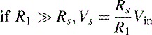
A Wheatstone bridge circuit is a very common improvement on the simple voltage divider. It consists simply of the same voltage divider as in Figure 2.1 combined with a second divider composed of fixed resistors only. The point of this additional divider is to make a reference voltage that is the same as the output of the sense voltage divider at some nominal value of the sense resistance. There are many complicated additional features that can be added to bridge circuits to more accurately compensate for particular effects, but for this discussion, we will concentrate on the simplest designs—the ones with a single sense resistor, and three other bridge resistors with resistance values that match the sense resistor at some nominal operating point (Figure 2.2).

Figure 2.2. Wheatstone bridge circuit.

The output of the sense divider and the reference divider are the same when the sense resistance is at its starting value, and changes in the sense resistance lead to small differences between these two voltages. A differential amplifier (such as an instrumentation amplifier) is used to produce the difference between these two voltages and amplify the result. The primary advantages are that there is very little offset voltage at the output of this differential amplifier and that temperature or other effects that are common to all the resistors are automatically compensated out of the resulting signal. Eliminating the offset means that the small differential signal at the output can be amplified without also amplifying an offset voltage, which makes the design of the rest of the circuit easier.

2.1.5.2. Capacitance measuring circuits

Many sensors respond to physical signals by producing a change in capacitance. How is capacitance measured? Essentially, all capacitors have an impedance given by

where f is the oscillation frequency in hertz, ω is in radians per second, and C is the capacitance in farads. The i in this equation is the square root of −1 and signifies the phase shift between the current through a capacitor and the voltage across the capacitor.

Now, ideal capacitors cannot pass current at DC, since there is a physical separation between the conductive elements. However, oscillating voltages induce charge oscillations on the plates of the capacitor, which act as if there is physical charge flowing through the circuit. Since the oscillation reverses direction before substantial charges accumulate, there are no problems. The effective resistance of the capacitor is a meaningful characteristic, as long as we are talking about oscillating voltages.

With this in mind, the capacitor looks very much like a resistor. Therefore, we may measure capacitance by building voltage divider circuits as in Figure 2.1, and we may use either a resistor or a capacitor as the load resistance. It is generally easiest to use a resistor, since inexpensive resistors are available that have much smaller temperature coefficients than any reference capacitor. Following this analogy, we may build capacitance bridges as well. The only substantial difference is that these circuits must be biased with oscillating voltages. Since the “resistance” of the capacitor depends on the frequency of the AC bias, it is important to select this frequency carefully. By doing so, all of the advantages of bridges for resistance measurement are also available for capacitance measurement.

However, providing an AC bias can be problematic. Moreover, converting the AC signal to a DC signal for a microprocessor interface can be a substantial issue. On the other hand, the availability of a modulated signal creates an opportunity for use of some advanced sampling and processing techniques. Generally speaking, voltage oscillations must be used to bias the sensor. They can also be used to trigger voltage sampling circuits in a way that automatically subtracts the voltages from opposite clock phases. Such a technique is very valuable, because signals that oscillate at the correct frequency are added up, while any noise signals at all other frequencies are subtracted away. One reason these circuits have become popular in recent years is that they can be easily designed and fabricated using ordinary digital VLSI fabrication tools. Clocks and switches are easily made from transistors in CMOS circuits. Therefore, such designs can be included at very small additional cost—remember that the oscillator circuit has to be there to bias the sensor anyway.

Capacitance measuring circuits are increasingly implemented as integrated clock/sample circuits of various kinds. Such circuits are capable of good capacitance measurement but not of very high performance measurement, since the clocked switches inject noise charges into the circuit. These injected charges result in voltage offsets and errors that are very difficult to eliminate entirely. Therefore, very accurate capacitance measurement still requires expensive precision circuitry.

Since most sensor capacitances are relatively small (100 pF is typical) and the measurement frequencies are in the 1–100 kHz range, these capacitors have impedances that are large (>1 MΩ is common). With these high impedances, it is easy for parasitic signals to enter the circuit before the amplifiers and create problems for extracting the measured signal. For capacitive measuring circuits, it is therefore important to minimize the physical separation between the capacitor and the first amplifier. For microsensors made from silicon, this problem can be solved by integrating the measuring circuit and the capacitance element on the same chip, as is done for the ADXL311 mentioned above.

2.1.5.3. Inductance Measurement Circuits

Inductances are also essentially resistive elements. The “resistance” of an inductor is given by X^L = 2πfL, and this resistance may be compared with the resistance of any other passive element in a divider circuit or in a bridge circuit, as shown in Figure 2.1. Inductive sensors generally require expensive techniques for the fabrication of the sensor mechanical structure, so inexpensive circuits are not generally of much use. In large part, this is because inductors are generally three-dimensional devices, consisting of a wire coiled around a form. As a result, inductive measuring circuits are most often of the traditional variety, relying on resistance divider approaches.

2.1.6. Sensor Limitations

2.1.6.1. Limitations in Resistance Measurement

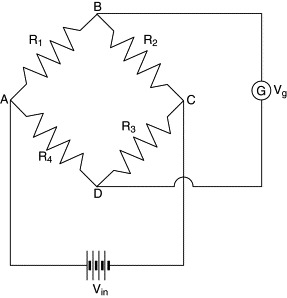
• Lead resistance—The wires leading from the resistive sensor element have a resistance of their own. These resistances may be large enough to add errors to the measurement, and they may have temperature dependencies that are large enough to matter. One useful solution to the problem is the use of the so-called four-wire resistance approach (Figure 2.3). In this case, current (from a current source, as in Figure 2.1) is passed through the leads and through the sensor element. A second pair of wires is independently attached to the sensor leads, and a voltage reading is made across these two wires alone. It is assumed that the voltage-measuring instrument does not draw significant current (see the next point), so it simply measures the voltage drop across the sensor element alone. Such a four-wire configuration is especially important when the sensor resistance is small, and the lead resistance is most likely to be a significant problem.

  Figure 2.3. Lead compensation.

  

• Output impedance—The measuring network has a characteristic resistance that, simply put, places a lower limit on the value of a resistance that may be connected across the output terminals without changing the output voltage. For example, if the thermistor resistance is 10 kΩ and the load resistor resistance is 1 MΩ, the output impedance of this circuit is approximately 10 kΩ. If a 1-kΩ resistor is connected across the output leads, the output voltage would be reduced by about 90%. This is because the load applied to the circuit (1 kΩ) is much smaller than the output impedance of the circuit (10 kΩ), and the output is “loaded down.” So, we must be concerned with the effective resistance of any measuring instrument that we might attach to the output of such a circuit. This is a well-known problem, so measuring instruments are often designed to offer maximum input impedance, so as to minimize loading effects. In our discussions we must be careful to arrange for instrument input impedance to be much greater than sensor output impedance.

2.1.6.2. Limitations to Measurement of Capacitance

Any wire in a real-world environment has a finite capacitance with respect to ground. If we have a sensor with an output that looks like a capacitor, we must be careful with the wires that run from the sensor to the rest of the circuit. These stray capacitances appear as additional capacitances in the measuring circuit and can cause errors. One source of error is the changes in capacitance that result from these wires moving about with respect to ground, causing capacitance fluctuations that might be confused with the signal. Since these effects can be due to acoustic pressure-induced vibrations in the positions of objects, they are often referred to as microphonics. An important way to minimize stray capacitances is to minimize the separation between the sensor element and the rest of the circuit. Another way to minimize the effects of stray capacitances is mentioned later, the virtual ground amplifier.

2.1.7. Filters

Electronic filters are important for separating signals from noise in a measurement. The following sections contain descriptions of several simple filters used in sensor-based systems.

• Low pass A low-pass filter (Figure 2.4) uses a resistor and a capacitor in a voltage divider configuration. In this case, the “resistance” of the capacitor decreases at high frequency, so the output voltage decreases as the input frequency increases. So, this circuit effectively filters out the high frequencies and “passes” the low frequencies.
  • The mathematical analysis is as follows. Using the complex notation for the impedance, let

    

  • Using the voltage divider equation in Figure 2.1,

    

  • Substituting for Z¹ and Z²,

    

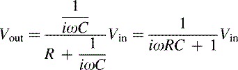
  • The magnitude of V^out is

    and the phase of V^out is

    

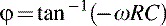
  Figure 2.4. Low-pass filter.

  

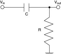
• High pass The high-pass filter is exactly analogous to the low-pass filter, except that the roles of the resistor and capacitor are reversed. The analysis of a high-pass filter, shown in Figure 2.5, is as follows. Similar to a low-pass filter,
  • The magnitude is

    and the phase is

    

  Figure 2.5. High-pass filter.

  

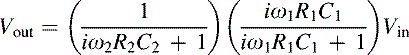
• Bandpass By combining low-pass and high-pass filters together, we can create a bandpass filter that allows signals between two preset oscillation frequencies (Figure 2.6). The derivations are as follows. Let the high-pass filter have the oscillation frequency ω¹ and the low-pass filter have the frequency ω² such that

  

  • Then the relation between V^out and Vⁱⁿ is

    

  • The operational amplifier in the middle of the circuit was added in this circuit to isolate the high-pass from the low-pass filter so that they do not effectively load each other. The op-amp simply works as a buffer in this case. In the following section, the role of the op-amps will be discussed more in detail.

  Figure 2.6. Bandpass filter.

  

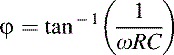
2.1.8. Operational Amplifiers

Operational amplifiers (op-amps) are electronic devices that are of enormous generic use for signal processing. The use of op-amps can be complicated, but there are a few simple rules and a few simple circuit building blocks that designers need to be familiar with to understand many common sensors and the circuits used with them.

An op-amp is essentially a simple two-input, one-output device. The output voltage is equal to the difference between the noninverting input and the inverting input multiplied by some extremely large value (10⁵). Use of op-amps as simple amplifiers is uncommon.

Feedback is a particularly valuable concept in op-amp applications. For instance, consider the circuit shown in Figure 2.7, called the follower configuration. Notice that the inverting input is tied directly to the output. In this case, if the output is less than the input, the difference between the inputs is a positive quantity, and the output voltage will be increased. This adjustment process continues, until the output is at the same voltage as the noninverting input. Then, everything stays fixed, and the output will follow the voltage of the noninverting input. This circuit appears to be useless until you consider that the input impedance of the op-amp can be as high as 10⁹Ω, while the output can be many orders of magnitude smaller. Therefore, this follower circuit is a good way to isolate circuit stages with high output impedance from stages with low input impedance.

Figure 2.7. Noninverting unity gain amplifier.

This op-amp circuit can be analyzed very easily, using the op-amp golden rules:

1. No current flows into the inputs of the op-amp.
2. When configured for negative feedback, the output will be at whatever value makes the input voltages equal.

Even though these golden rules only apply to ideal operational amplifiers, op-amps can in most cases be treated as ideal. Let us use these rules to analyze more circuits.

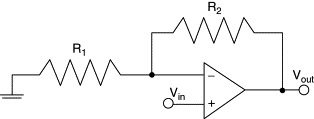
Figure 2.8 shows an example of an inverting amplifier. We can derive the equation by taking the following steps:

1. Point B is ground. Therefore, point A is also ground (Rule 2)
2. Since the current flowing from Vⁱⁿ to V^out is constant (Rule 1), V^out/R² = –Vⁱⁿ/R¹
3. Therefore, voltage gain = V^out/Vⁱⁿ = –R²/R¹

Figure 2.8. Inverting amplifier.

Figure 2.9 illustrates another useful configuration of an op-amp. This is a noninverting amplifier, which is a slightly different expression than the inverting amplifier. Taking it step-by-step,

1. V^a = Vⁱⁿ (Rule 2)
2. Since V^a comes from a voltage divider, V^a = [R¹/(R¹ + R²)] V^out
3. Therefore, Vⁱⁿ = [R¹/(R¹ + R²)] V^out
4. V^out/Vⁱⁿ = (R¹ + R²)/R¹ = 1 + R²/R¹

Figure 2.9. Noninverting amplifier.

The following section provides more details on sensor systems and signal conditioning.

2.2. Sensor Systems

This section deals with sensors and associated signal conditioning circuits. The topic is broad, but the focus here is to concentrate on the sensors with just enough coverage of signal conditioning to introduce it and to at least imply its importance in the overall system.

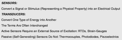
Strictly speaking, a sensor is a device that receives a signal or stimulus and responds with an electrical signal, while a transducer is a converter of one type of energy into another (Figure 2.10). In practice, however, the terms are often used interchangeably.

Figure 2.10. Sensor overview.

Sensors and their associated circuits are used to measure various physical properties, such as temperature, force, pressure, flow, position, and light intensity. These properties act as the stimulus to the sensor, and the sensor output is conditioned and processed to provide the corresponding measurement of the physical property. We will not cover all possible types of sensors here, only the most popular ones, and specifically, those that lend themselves to process control and data acquisition systems.

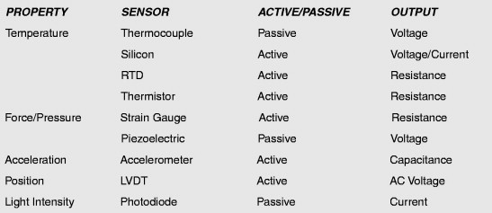
Sensors do not operate by themselves. They are generally part of a larger system consisting of signal conditioners and various analog or digital signal processing circuits (Figure 2.11). The system could be a measurement system, data acquisition system, or process control system, for example.

Figure 2.11. Typical sensors and their outputs.

Sensors may be classified in a number of ways. From a signal conditioning viewpoint it is useful to classify sensors as either active or passive. An active sensor requires an external source of excitation. Resistor-based sensors such as thermistors, RTDs (resistance temperature detectors), and strain gauges are examples of active sensors, because a current must be passed through them and the corresponding voltage measured in order to determine the resistance value. An alternative would be to place the devices in a bridge circuit; however, in either case, an external current or voltage is required.

On the other hand, passive (or self-generating) sensors generate their own electrical output signal without requiring external voltages or currents. Examples of passive sensors are thermocouples and photodiodes, which generate thermoelectric voltages and photocurrents, respectively, that are independent of external circuits. It should be noted that these definitions (active vs. passive) refer to the need (or lack thereof) of external active circuitry to produce the electrical output signal from the sensor. It would seem equally logical to consider a thermocouple to be active in the sense that it produces an output voltage with no external circuitry. However, the convention in the industry is to classify the sensor with respect to the external circuit requirement as defined previously.

A logical way to classify sensors is with respect to the physical property the sensor is designed to measure. Thus, we have temperature sensors, force sensors, pressure sensors, motion sensors, and so on. However, sensors that measure different properties may have the same type of electrical output. For instance, a resistance temperature detector is a variable resistance sensor, as is a resistive strain gauge. Both RTDs and strain gauges are often placed in bridge circuits, and the conditioning circuits are therefore quite similar. In fact, bridges and their conditioning circuits deserve a detailed discussion.

The full-scale outputs of most sensors (passive or active) are relatively small voltages, currents, or resistance changes; and therefore their outputs must be properly conditioned before further analog or digital processing can occur. Because of this, an entire class of circuits has evolved, generally referred to as signal conditioning circuits. Amplification, level translation, galvanic isolation, impedance transformation, linearization, and filtering are fundamental signal conditioning functions that may be required.

Whatever form the conditioning takes, however, the circuitry and performance will be governed by the electrical character of the sensor and its output. Accurate characterization of the sensor in terms of parameters appropriate to the application, such as sensitivity, voltage and current levels, linearity, impedances, gain, offset, drift, time constants, maximum electrical ratings, stray impedances, and other important considerations, can spell the difference between substandard and successful application of the device, especially in cases where high resolution and precision, or low-level measurements are involved.

Higher levels of integration now allow ICs to play a significant role in both analog and digital signal conditioning. ADCs (analog-to-digital converters) specifically designed for measurement applications often contain on-chip programmable-gain amplifiers (PGAs) and other useful circuits, such as current sources for driving RTDs, thereby minimizing the external conditioning circuit requirements.

Most sensor outputs are nonlinear with respect to the stimulus, and their outputs must be linearized to yield correct measurements. Analog techniques may be used to perform this function. However, the recent introduction of high-performance ADCs now allows linearization to be done much more efficiently and accurately in software and eliminates the need for tedious manual calibration using multiple and sometimes interactive trim pots.

The application of sensors in a typical process control system is shown in Figure 2.12. Assume the physical property to be controlled is the temperature. The output of the temperature sensor is conditioned and then digitized by an ADC. The microcontroller or host computer determines if the temperature is above or below the desired value and outputs a digital word to the digital-to-analog converter (DAC). The DAC output is conditioned and drives the actuator, in this case a heater. Notice that the interface between the control center and the remote process is via the industry-standard 4–20-mA loop.

Figure 2.12. Typical industrial process control loop.

Digital techniques have become increasingly popular in processing sensor outputs in data acquisition, process control, and measurement. Generally, 8-bit microcontrollers (8051-based, for example) have sufficient speed and processing capability for most applications. By including the A/D conversion and the microcontroller programmability on the sensor itself, a “smart sensor” can be implemented with self-contained calibration and linearization features, among others. A smart sensor can then interface directly to an industrial network as shown in Figure 2.13.

Figure 2.13. Standardization at the digital interface using smart sensors.

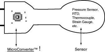
The basic building blocks of a “smart sensor” are shown in Figure 2.14, constructed with multiple ICs. The Analog Devices MicroConverter™ series of products includes on-chip high-performance multiplexers, analog-to-digital converters, and digital-to-analog converters, coupled with flash memory and an industry-standard 8052 microcontroller core, as well as support circuitry and several standard serial port configurations. These are the first integrated circuits that are truly smart sensor data acquisition systems (high-performance data conversion circuits, microcontroller, flash memory) on a single chip (see Figure 2.15).

Figure 2.14. Basic elements in a smart sensor.

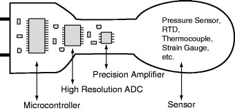
Figure 2.15. The even smarter sensor.

2.3. Application Considerations

The highest-quality, most up-to-date, most accurately calibrated, and most carefully selected sensor can still give totally erroneous data if it is not correctly applied. This section will address some of the issues that need to be considered to assure correct application of any sensor.

The following checklist is derived from a list originally assembled by Applications Engineering at Endevco^® in the late 1970s. It has been sporadically updated as additional issues were encountered. It is generally applicable to all sensor applications, but many of the items mentioned will not apply to any given specific application. However, it provides a reminder of questions that need to be asked and answered during selection and application of any sensor.

Often one of the most difficult tasks facing an instrumentation engineer is the selection of the proper measuring system. Economic realities and the pressing need for safe, properly functioning hardware create an ever-increasing demand to obtain accurate, reliable data on each and every measurement.

On the other hand, each application will have different characteristics from the next and will probably be subjected to different environments with different data requirements. As test or measurement programs progress, data are usually subjected to increasing manipulation, analysis, and scrutiny. In this environment, the instrumentation engineer can no longer depend on general-purpose measurement systems and expect to obtain acceptable data. Indeed, he or she must carefully analyze every aspect of the test to be performed, the test article, the environmental conditions, and if available, the analytical predictions. In most cases, this process will indicate a clear choice of acceptable system components. In some cases, this analysis will identify unavoidable compromises or trade-offs and alert the instrumentation engineer and the customer to possible deficiencies in the results.

The intent of this chapter is to assist in the process of selecting an acceptable measuring system. While we hope it will be an aid, we understand it cannot totally address the wide variety of situations likely to arise.

Let us look at a few hypothetical cases where instrument selection was made with care, but where the tests were failures.

1. A test requires that low acceleration of gravity, low-frequency information be measured on the axle bearings of railroad cars to assess the state of the roadbed. After considerable evaluation of the range of conditions to be measured, a high-sensitivity, low-resonance piezoelectric accelerometer is selected. The shocks generated when the wheels hit the gaps between track sections saturate the amplifier, making it impossible to gather any meaningful data.
2. A test article must be exposed to a combined environment of vibration and a rapidly changing temperature. The engineer selects an accelerometer for its high temperature rating without consulting the manufacturer. Thermal transient output swamps the vibration data.
3. Concern over ground loops prompts the selection of an isolated accelerometer. The test structure is made partially from lightweight composites, and the cases of some accelerometers are not referenced to ground. Capacitive coupling of radiated interference to the signal line overwhelms the data.

From these examples, we hope to make the point that, for all measurement systems, it is not adequate to consider only that which we wish to measure. In fact, every physical and electrical phenomenon present needs to be considered lest it overwhelm or, perhaps worse, subtly contaminate our data. The user must remember that every measurement system responds to its total environment.

2.4. Sensor Characteristics

The prospective user is generally forced to make a selection based on the characteristics available on the product data sheet. Many performance characteristics are shown on a typical data sheet. Many manufacturers feel that the data sheet should provide as much information as possible. Unfortunately, this abundance of data may create some confusion for a potential user, particularly the new user. Therefore the instrumentation engineer must be sure he or she understands the pertinent characteristics and how they will affect the measurement. If there is any doubt, the manufacturer should be contacted for clarification.

2.5. System Characteristics

The sensor and signal conditioners must be selected to work together as a system. Moreover, the system must be selected to perform well in the intended applications. Overall system accuracy is usually affected most by sensor characteristics such as environmental effects and dynamic characteristics. Amplifier characteristics such as nonlinearity, harmonic distortion, and flatness of the frequency response curve are usually negligible when compared to sensor errors.

2.6. Instrument Selection

Selecting a sensor/signal conditioner system for highly accurate measurements requires very skillful and careful measurement engineering. All environmental, mechanical, and measurement conditions must be considered. Installation must be carefully planned and carried out. The following guidelines are offered as an aid to selecting and installing measurement systems for the best possible accuracy.

2.6.1. Sensor

The most important element in a measurement system is the sensor. If the data are distorted or corrupted by the sensor, there is often little that can be done to correct it.

Will the sensor operate satisfactorily in the measurement environment? Check:

• Temperature range
• Maximum shock and vibration
• Humidity
• Pressure
• Acoustic level
• Corrosive gases
• Magnetic and RF fields
• Nuclear radiation
• Salt spray
• Transient temperatures
• Strain in the mounting surface

Will the sensor characteristics provide the desired data accuracy? Check:

• Sensitivity
• Frequency response: resonance frequency, minor resonances
• Internal capacitance
• Transverse sensitivity
• Amplitude linearity and hysteresis
• Temperature deviation
• Weight and size
• Internal resistance at maximum temperature
• Calibration accuracy
• Strain sensitivity
• Damping at temperature extremes
• Zero measurand output
• Thermal zero shift
• Thermal transient response

Is the proper mounting being used for this application? Check:

• Is an insulating stud required? Ground loops? Calibration simulation?
• Is adhesive mounting required? Thread size, depth, and class?

2.6.2. Cable

Cables and connectors are usually the weakest link in the measurement system chain.

Will the cable operate satisfactorily in the measurement environment? Check:

• Temperature range
• Humidity conditions

Will the cable characteristics provide the desired data accuracy? Check:

• Low noise
• Size and weight
• Flexibility
• Is sealed connection required?

2.6.3. Power Supply

Will the power supply operate satisfactorily in the measurement environment? Check:

• Temperature range
• Maximum shock and vibration
• Humidity
• Pressure
• Acoustic level
• Corrosive gases
• Magnetic and RF fields
• Nuclear radiation
• Salt spray

Is this the proper power supply for the application? Check:

• Voltage regulation
• Current regulation
• Compliance voltage: Output voltage adjustable? Output current adjustable?
• Long output lines? Need for external sensing?
• Isolation
• Mode card, if required

Will the power supply characteristics provide the desired data accuracy? Check:

• Load regulation
• Line regulation
• Temperature stability
• Time stability
• Ripple and noise
• Output impedance
• Line-transient response
• Noise to ground
• DC isolation

2.6.4. Amplifier

The amplifier must provide gain, impedance matching, output drive current, and other signal processing.

Will the amplifier operate satisfactorily in the measurement environment? Check:

• Temperature range
• Maximum shock and vibration
• Humidity
• Pressure
• Acoustic level
• Corrosive gases
• Magnetic and RF fields
• Nuclear radiation
• Salt spray

Is this the proper amplifier for the application? Check:

• Long input lines: Need for charge amplifier? Need for remote charge amplifier?
• Long output lines: Need for power amplifier?
• Airborne: Size, weight, power limitations

Will the amplifier characteristics provide the desired data accuracy? Check:

• Gain and gain stability
• Frequency response
• Linearity
• Stability
• Phase shift
• Output current and voltage
• Residual noise
• Input impedance
• Transient response
• Overload capability
• Common mode rejection
• Zero-temperature coefficient
• Gain-temperature coefficient

2.7. Data Acquisition and Readout

Does the remainder of the system, including any additional amplifiers, filters, and data acquisition and readout devices, introduce any limitation that will tend to degrade the sensor-amplifier characteristics?

Check all previous check items plus adequate resolution.

2.8. Installation

Even the most carefully and thoughtfully selected and calibrated system can produce bad data if carelessly or ignorantly installed.

2.8.1. Sensor

Is the unit in good condition and ready to use? Check:

• Up-to-date calibration
• Physical condition: Case, mounting surface, connector, mounting hardware
• Inspect for clean connector
• Internal resistance

Is the mounting hardware in good condition and ready to use? Check:

• Mounting surface condition
• Thread condition
• Burred end slots
• Insulated stud: Insulation resistance, stud damage by overtorquing
• Mounting surface clean and flat
• Sensor base surface clean and flat
• Hole drilled and tapped deep enough
• Correct tap size
• Hole properly aligned perpendicular to mounting surface
• Stud threads lubricated
• Sensor mounted with recommended torque

2.8.2. Cement Mounting

Check:

• Mounting surface clean and flat
• Dental cement for uneven surfaces
• Cement cured properly
• Sensor mounted to cementing stud with recommended torque

2.8.3. Cable

Is the cable in good condition and ready for use? Check:

• Physical condition: Cable kinked or crushed, connector threads and pins
• Inspect for clean connectors
• Continuity
• Insulation resistance
• Capacitance
• All cable connections secure
• Cable properly restrained
• Excess cable coiled and tied down
• Drip loop provided
• Connectors sealed and potted, if required

2.8.4. Power Supply, Amplifier, and Readout

Are the units in good condition and ready to use? Check:

• Up-to-date calibration
• Physical condition: Connectors, case, output cables
• Inspect for clean connectors
• Mounted securely
• All cable connections secure
• Gain hole cover sealed, if required
• Recommended grounding in use

When these questions have been answered to the user's satisfaction, the measurement system has a high probability of providing accurate data.

2.9. Measurement Issues and Criteria

Sensors are most commonly used to make quantifiable measurements, as opposed to qualitative detection or presence sensing. Therefore, it should be obvious that the requirements of the measurement will determine the selection and application of the sensor. How then can we quantify the requirements of the measurement?

First, we must consider what it is we want to measure. Sensors are available to measure almost anything you can think of and many things you would never think of (but someone has!). Pressure, temperature, and flow are probably the most common measurements, as they are involved in monitoring and controlling many industrial processes and material transfers. A brief tour of a Sensors Expo exhibition or a quick look at the Internet will yield hundreds, if not thousands, of quantities, characteristics, or phenomena that can be measured with sensors.

Second, we must consider the environment of the sensor. Environmental effects are perhaps the biggest contributor to measurement errors in most measurement systems. Sensors, and indeed whole measurement systems, respond to their total environment, not just to the measurand. In extreme cases, the response to the combination of environments may be greater than the response to the desired measurand. One of the sensor designer's greatest challenges is to minimize the response to the environment and maximize the response to the desired measurand. Assessing the environment and estimating its effect on the measurement system is an extremely important part of the selection and application process.

The environment includes not only such parameters as temperature, pressure, and vibration but also the mounting or attachment of the sensor, electromagnetic and electrostatic effects and the rates of change of the various environments. For example, a sensor may be little affected by extreme temperatures but may produce huge errors in a rapidly changing temperature (“thermal transient sensitivity”).

Third, we must consider the requirements for accuracy (uncertainty) of the measurement. Often, we would like to achieve the lowest possible uncertainty, but that may not be economically feasible or even necessary. How will the information derived from the measurement be used? Will it really make a difference, in the long run, whether the uncertainty is 1% or 1½%? Will highly accurate sensor data be obscured by inaccuracies in the signal conditioning or recording processes? On the other hand, many modern data acquisition systems are capable of much greater accuracy than the sensors making the measurement. A user must not be misled by thinking that high resolution in a data acquisition system will produce high-accuracy data from a low-accuracy sensor.

Last, but not least, the user must assure that the whole system is calibrated and traceable to a national standards organization (such as National Institute of Standards and Technology in the United States). Without documented traceability, the uncertainty of any measurement is unknown. Either each part of the measurement system must be calibrated and an overall uncertainty calculated or the total system must be calibrated as it will be used (“system calibration” or “end-to-end calibration”).

Since most sensors do not have any adjustment capability for conventional “calibration,” a characterization or evaluation of sensor parameters is most often required. For the lowest uncertainty in the measurement, the characterization should be done with the mounting and environment as similar as possible to the actual measurement conditions.

While this handbook concentrates on sensor technology, a properly selected, calibrated, and applied sensor is necessary but not sufficient to assure accurate measurements. The sensor must be carefully matched with, and integrated into, the total measurement system and its environment.